Parity oscillations of Kondo temperature in a single molecule break junction

Abstract

We study the Kondo temperature ($T_{K}$) of a single molecule break junction. By employing a numerical renormalization group calculations we have found that $T_{K}$ depends dramatically upon the position of the molecule in the wire formed between the contacts. We show that $T_{K}$ exhibits strong oscillations when the parity of the left and/or right number of atomic sites ($N_{L},N_{R}$) is changed. For a given set of parameters, the maximum value of $T_{K}$ occurs for ($odd,odd$) combination, while its minimum values is observed for ($even,even$). These oscillations are fully understood in terms of the effective hybridization function.

Kondo effect (KE) is one of the most intriguing phenomena of strong correlated systems,Hewson-Kondo which was beautifully explained by J. Kondo in the 60’s in the seminal theoretical work on the minimal resistance in magnetic alloys.Prog.Theor.Phys…32 KE has revived in the later 90’s with the advent of the scanning tunneling microscope (STM) that has facilitated the manipulation of the matter at atomic scale. For instance, STM has allowed observation of interesting facets of the KE in quantum dots (QD)Nature.391.156 ; *Science.S.1998.540 and in single atom or molecule on metallic surfaces,Sicence.280.567 ; Nature.403.512 ; PhysRevLett.97.266603 which have motivated a huge number of experimentalNature.391.156 ; Science.S.1998.540 ; Sicence.268.1440 ; *Science.293.2221 and theoreticalPhysRevLett.82.3508 ; PhysRevB.78.054445 investigations.

One of the experimentally accessible signatures of the KE in nanoscopic system such as QD or magnetic molecules attached to metallic contacts is the strong modification in the conductance across the system, observable when the system is cooled down below the so-called Kondo temperature ($T_{K}$). In QD, for instance, $T_{K}$ is found to be in the sub Kelvin region whereas for large molecules attached to metallic leads $T_{K}$ can be much larger.PhysRevLett.97.266603 In both cases, in the limit of very strong Coulomb interaction, $T_{K}$ depends strongly upon the effective hybridization ($\Delta$) that connects the localized magnetic moments to the conduction electronsPhysRevLett.97.096603 ; PhysRevLett.97.266603 asHewson-Kondo $T_{K}\sim\exp({\pi\varepsilon_{d}/\Delta})$, where $\varepsilon_{d}$ ($<0$) is the energy of the localized orbital respect to the Fermi level. Controlling $\Delta$ or $\varepsilon_{d}$ is therefore crucial for obtaining higher $T_{K}$, which is fundamental for possible technological application of KE. While tuning $\varepsilon_{d}$ is relatively simple in QDs by mean of gate voltages, in molecules, on the other hand, it becomes a more complicated task. Conversely, geometrical parameters are more suitably modified in molecules than in QDs and has proven to produce important modifications in $T_{K}$ via hybridization function.PhysRevLett.99.026601

A suitable experimental arrangement to study the KE is the break junction (BJ) molecular structures, in which a metallic wire (gold wire, for instance) is stretched until a few-atom 1D chain bridges the gap between the electrodes before the complete break up of the wire.PhysRevLett.87.096803 ; NatureCommunications.2.305 ; NatureNanotechnology.1.173 ; Nature.419.906 ; PhysRevLett.91.076805 Owing to the dependence of $T_{K}$ upon $\Delta$ it has been shown that $T_{K}$ can be mechanically modulated in BJ experimentsPhysRevLett.99.026601 by changing the distance between the electrodes. Motivated by this experiment, in the present work we study the Kondo temperature of a spin-$1/2$ magnetic impurity coupled to metallic contacts through two finite (left and right) quantum wires (QW), as illustrated in Fig. 1(a). By employing a numerical renormalization groupRevModPhys.47.773 ; RevModPhys.80.395 (NRG) calculation we find a strong dependence of $T_{K}$ upon the parity of the number of sites ($N_{R},N_{L}$) of each QW as well as their length. The dependence upon the ($N_{L},N_{R}$) parity combination results in an oscillating behavior of $T_{K}$ as function of $N_{L}$ or $N_{R}$, akin to what has been observed in Manganese phthalocyanine (MnPc) molecules on top of Pb islands, reported in Ref. PhysRevLett.99.256601, . Although the system under investigation here is quite different from the one studied in Ref. PhysRevLett.99.256601, , the origin of the oscillation of $T_{K}$ can be interpreted likewise. While in their case the enhancement of $\Delta$ originates from the formation of multiple quantum well states between the Pb atomic layers, here the enhancement of $\Delta$ results from the localized states of the atomic sites of the QW.

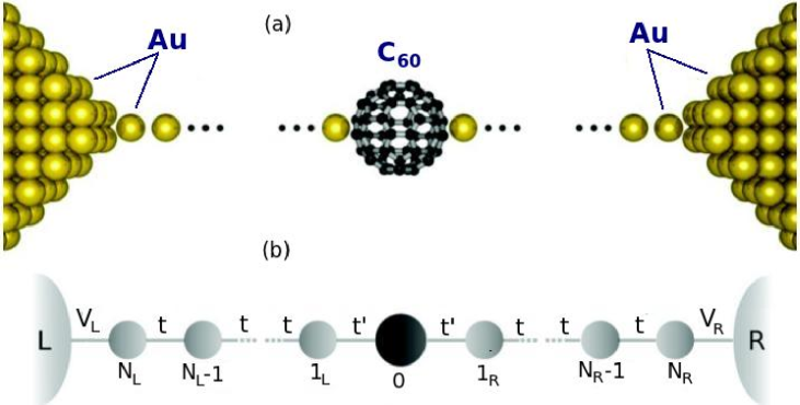
Figure 1: (Color online) (a) Illustration of a Au quantum wire coupled to metallic contacts with a embedded C₆₀ molecule. (b) Pictorial representation of the model. The site labeled as “0” represents the impurity site with strong on-site coulomb repulsion.

Our system model is schematically represented in Fig. 1(b) and is modeled by the Anderson-type Hamiltonian that can be split into five terms as

$$H=H_{imp}+H_{cb}+H_{wires}+H_{imp-wires}+H_{cbs-wires},$$ (1)

where $H_{imp}$, $H_{cb}$ and $H_{wires}$ describe, respectively, the interacting impurity, the free electrons in the conduction bands and the electrons in the wires, $H_{imp-wires}$ couples the impurity to the two wires and $H_{cb-wires}$ couples the wires the their respective conduction bands. In terms of creation and annihilation fermion operators the Hamiltonians read

$$H_{imp} = \sum_{\sigma}\varepsilon_{d}c^{\dagger}_{d\sigma}c_{d\sigma}+Un_{d\uparrow}n_{d\downarrow},$$ (2)

$$H_{cb} = \sum_{\ell=R,L}\sum_{k\sigma}\varepsilon_{k}c^{\dagger}_{\ell k\sigma}c_{\ell k\sigma}$$ (3)

$$H_{wires} = \sum_{\ell=R,L}\left[{\color[rgb]{0,0,0}\varepsilon_{0}\sum_{i_{\ell}=1\atop\sigma}^{N_{\ell}}n_{i_{\ell}\sigma}+}t\sum_{i_{\ell}=1\atop\sigma}^{N_{\ell}-1}\left(c^{\dagger}_{i_{\ell}\sigma}c_{i_{\ell}+1}+H.c.\right)\right],$$ (4)

$$H_{cb-wires} = \sum_{\ell=R,L}\sum_{\ell k\sigma}\left(V_{\ell k}c^{\dagger}_{N_{\ell}}c_{\ell k\sigma}+V^{*}_{\ell k}c^{\dagger}_{\ell k\sigma}c_{N_{\ell}}\right)$$ (5)

$$H_{imp-wires} = t^{\prime}\sum_{\ell=R,L}\sum_{\ell\sigma}\left(c^{\dagger}_{d\sigma}c_{1_{\ell}}+c^{\dagger}_{1_{\ell}\sigma}c_{d\sigma}\right).$$ (6)

In Eqs. 2-6, the operators $c^{\dagger}_{d\sigma}$ ($c_{d\sigma}$) creates (annihilates) an electron in the orbital $d$ with energy $\varepsilon_{d}$, $c^{\dagger}_{\ell k\sigma}$ ($c_{\ell k\sigma}$) creates (annihilates) an electron in the $\ell$th conduction band with energy $\varepsilon_{k}$, $c^{\dagger}_{i_{\ell}\sigma}$ ($c_{i_{\ell}\sigma}$) creates (annihilates) and electron in the $i$th site of the $\ell$th QW with energy $\varepsilon_{0}$ spin $\sigma$. Finally, $t$ is the hopping between two adjacent sites in the wires and $V_{\ell k}$ and $t^{\prime}$ couple the QWs to their conduction bands and to the impurity, respectively. The conduction bands are characterized by a flat density of states, $\rho(\omega)=(1/2D)\Theta(D-|\omega|)$, where $D$ is their half bandwidth and $\Theta(x)$ is the Heaviside step function. It is worth emphasizing that although the motivating experiment was realized using C₆₀ molecule coupled to Au metallic contacts, this model is rather general. In the particular context of molecular BJ, vibrations may be important in certain range of parameters, but this aspect is beyond the scope of the present work.

In order to properly address the Kondo physics of the system, the full Hamiltonian is approached by using the numerical renormalization method, with which we can calculate the thermodynamical properties. Within the NRG approach we discretize the effective conduction band “seen” by the interacting impurity. The effective conduction band can be determined by exact calculation of the local non-interacting ($U=0$) Green’s function (suppressing the spin index), $g_{dd}(\omega)=[\omega-\epsilon_{d}+\Sigma(\omega)]^{-1}$, where $\Sigma=\Sigma_{R}(\omega)+\Sigma_{L}(\omega)$, in which the $\ell$th self-energy is given by

$$\Sigma_{\ell}(\omega)=-\cfrac{t^{\prime 2}}{\omega-\cfrac{t^{2}}{\omega-\cfrac{t^{2}}{\omega-\cfrac{t^{2}}{\cfrac{\ddots t^{2}}{\omega-V_{\ell}^{2}\tilde{g}(\omega)}}}}},$$ (7)

with

$$\tilde{g}(\omega)=-\frac{1}{2D}\ln\Big{|}\frac{\omega-D}{\omega+D}\Big{|}-\frac{i\pi}{2D}\Theta(D-|\omega|)$$ (8)

being the diagonal GF associated to the unperturbed conduction electrons in the leads. The fraction in Eq. 7 is continued until all the sites of the of the $\ell$th wire and the $\ell$th conduction band are taken into account.

The hybridization of the localized orbital “$d$” with the effective band is give by $\Delta(\omega)={\tt Im}[\Sigma(\omega)]=\Delta_{L}(\omega)+\Delta_{R}(\omega)$ [Hereafter we will refers to $\Delta(0)$ just as $\Delta$]. The hybridization function is logarithmically discretizedRevModPhys.80.395 ; PhysRevB.52.14436 to map the system in a Wilson’s chain form,RevModPhys.47.773

$$H=H_{imp}+t^{\prime}\sum_{\sigma}\left(c^{\dagger}_{d\sigma}c_{0\sigma}+c^{\dagger}_{0\sigma}c_{d\sigma}\right)+\sum_{i=0\atop\sigma}^{\infty}\varepsilon_{i\sigma}c^{\dagger}_{i\sigma}c_{i\sigma}$$

$$+\sum_{i=0\atop\sigma}^{\infty}t_{i}\left(c^{\dagger}_{i\sigma}c_{i+1\sigma}+c^{\dagger}_{i+1\sigma}c_{i\sigma}\right),$$ (9)

where $t_{i}$’s are calculated via $\Delta(\omega)$, following the recipes described in Ref. PhysRevB.52.14436, . Once we have mapped the system in the Wilson’s form, we proceed the NRG calculation, which is based in the iterative diagonalization of the effective Hamiltonian.RevModPhys.80.395 After reaching the strong coupling fixed point we can calculate the magnetic moment within the canonical ensemble as

$$k_{B}T\chi(T)=\frac{1}{Z(T)}\sum_{\nu}\left[\langle\nu|S^{2}_{z}|\nu\rangle-(\nu|S_{z}|\nu\rangle)^{2}\right]e^{-E_{\nu}/k_{B}T},$$ (10)

where $k_{B}$ is the Boltzmann constant, $Z(T)=\sum_{\nu}\exp(-E_{\nu}/k_{B}T)$ is the canonical partition function, $S_{z}$ is the spin operator, $|\nu\rangle$ and $E_{\nu}$ are, respectively, the eigenvector and its corresponding eigenvalue of the full interacting Hamiltonian, which are naturally calculated in the NRG procedure. Following Wilson’s criterion, we define $T_{K}$ from the “impurity” magnetic moment as $k_{B}T_{K}\chi_{imp}(T_{K})=0.0707(g\mu_{B})^{2}$, (that is the magnetic moment of the full system subtracted by the contribution of the effective conduction band), $g$ is the electron $g$-factor and $\mu_{B}$ is the Bohr magneton.

Before starting the presentation of our numerical results, lets analyze the hybridization function at the Fermi level, which is the most relevant parameter to determine the behavior of $T_{K}$ in our calculations. It is straightforward to show from Eq. 7 that $\Delta$ possesses only three distinct vales,

$$\Delta=\left\{\begin{array}[]{cc}\Delta_{min}=\Delta_{0}&\quad\mbox{for (even,even)}\\ \Delta_{int}=\Delta_{0}\left(\frac{1}{2}+\alpha\right)&\quad\mbox{for (even,odd) or (odd,even)}\\ \Delta_{max}=2\alpha\Delta_{0}&\quad\mbox{for (odd,odd)}\end{array}\right.,$$ (11)

where we have defined $\Delta_{0}=\pi t^{\prime 2}/D$ and denoted $\Delta_{min}$, $\Delta_{int}$ and $\Delta_{max}$, the minimum, intermediate and maximum value of $\Delta$, respectively, and $\alpha=2(D/\pi t)^{2}$ is a dimensionless parameter that can be modified, for instance, by stretching the QW as is was done in the Ref. PhysRevLett.99.026601, . To obtain our numerical results lets set $D=1$ as our energy scale. With that we choose hereafter (unless otherwise stated) $U=0.5$, $\epsilon_{d}=-0.25$, $\varepsilon_{0}=0$ (at the particle-hole symmetric point), $V_{R}=V_{L}=t=0.15$ and $t^{\prime}=0.1$.

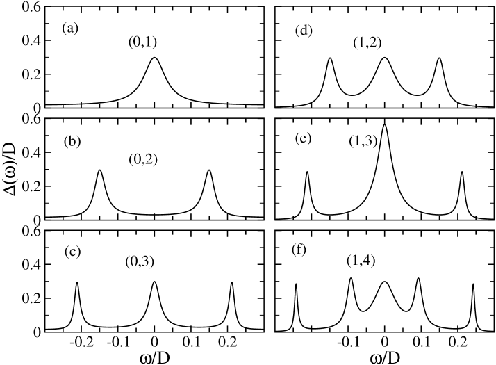
Figure 2: (Color online) Hybridization function vs energy for various values of $N_{L}$ and $N_{L}$ [denoted in the figure as ($N_{L},N_{R}$) using $V_{L}=V_{R}=t=0.15$ and $t^{\prime}=0.1$. Notice that $\Delta$ possesses three different values, depending on the parity of $N_{L}$ and $N_{R}$. The minimum ($\Delta_{min}$) and maximum ($\Delta_{max}$) value of $\Delta$ is obtained for $(even,even)$ (b) and $(odd,odd)$ (e), respectively, while for all the other combinations $\Delta$ has an intermediate value, $\Delta_{int}$.

In Fig. 2 we show the hybridization function vs energy for various values of $N_{L}$ and $N_{R}$. In Figs. 2(a), 2(b), and 2(c) we fix $N_{L}=0$ and show $\Delta(\omega)$ for $N_{R}=1$, $N_{R}=2$ and $N_{R}=3$, while in Figs. 2(d), 2(e), and 2(f) we keep $N_{L}=1$ fixed and show $\Delta(\omega)$ for $N_{R}=2$, $N_{R}=3$ and $N_{R}=4$. The number of peaks of $\Delta(\omega)$ is given by $\max(N_{L},N_{R})$ for equal parity and $N_{R}+N_{L}$ for different parities. Although the structure of $\Delta(\omega)$ away from the Fermi level has some effect on $T_{K}$, the most relevant contribution comes from the structures at or very close the the Fermi level. For the parameters set above, we obtain $\Delta_{min}\approx 0.0314$, $\Delta_{max}\approx 0.566$ and $\Delta_{int}\approx 0.299$. These distinct values of $\Delta$ are crucial for determining the Kondo temperature of the system, which in our case can be roughly estimated asPhysRevB.21.1003 $k_{B}T_{K}(\Delta)\sim\exp[-\pi U/8\Delta]$. It is clear that $T_{K}$ increases as $\Delta$ increases.

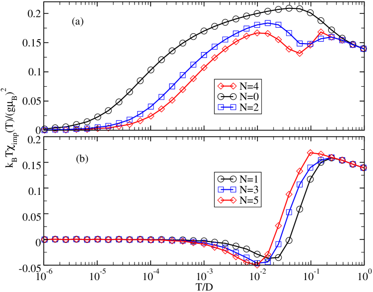
Figure 3: (Color online) Magnetic moment as function of temperature for various values of $N_{R}=N_{L}=N$. Panel (a) and (b) correspond to $N$ even and odd, respectively (see values of $N$ in the legends).

In Fig. 3(a) and Fig. 3(b) we show the magnetic moment as function temperature for various values of $N=N_{L}=N_{R}$ (the symmetric case) even and odd, respectively. The case of $N=0$ [Fig. 3(a), $\Circle$ (black)] corresponds to the single impurity coupled to two conduction band. The low temperature suppression in the magnetic moment results from the Kondo screening of the local spin [these curves are used to $T_{K}$, as discussed above]. On the other hand, in the high temperature limit the $k_{B}T\chi\rightarrow(g\mu_{B})^{2}/8$, as expected. Notice in Fig. 3(a) that $T_{K}$ increases when $N$ (even) increases. Conversely, $T_{K}$ decreases when $N$ (odd) increases as seen in Fig. 3(b). Notice also that $T_{K}$ can be at least two order of magnitude larger for $N$ odd than for $N$ even. This huge difference will be analyze below. The result for $N=1$ [Fig. 3(b), $\Circle$ (black)] is equivalent to those reported in Ref. PhysRevLett.97.096603, . The negative values of $k_{B}T\chi_{imp}$ within a small range of $T$ results from the subtraction of the effective conduction band contribution.

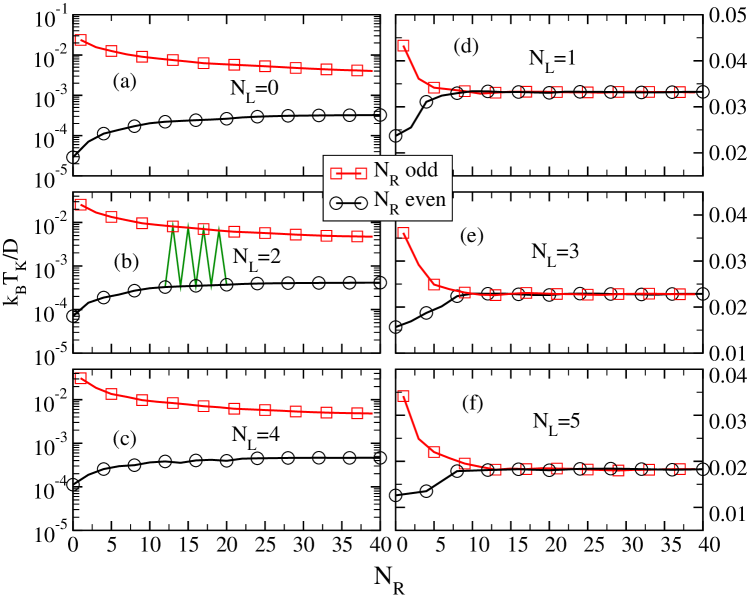
Figure 4: (Color online) Kondo temperature as function of number of sites ($N_{R}$) for a fixed $N_{L}=1$. $\Circle$ (black) and $\square$ (red) correspond to even (odd) $N_{R}$, respectively. The zig-zag (green) line shows the ($even,odd$) oscillation, similar to those observed in Ref. PhysRevLett.99.256601, .

In order to show the behavior of the Kondo temperature for larger and different values of $N_{L}$ and $N_{R}$ we show in Fig. 4 $T_{K}$ as function of $N_{R}$ for a fixed number $N_{L}$ even (left) and $N_{L}$ odd (right). The $\Circle$ (black) curves correspond to $N_{R}$ even, while $\square$ (red) curves corresponds to $N_{R}$ odd. Notice that for $N_{L}$ even [(Fig. 4(a), 4(b) and 4(c)] $T_{K}$ increases with $N_{R}$ even [$\Circle$ (black)] while it decreases for $N_{R}$ odd [$\square$ (red)]. Observe again that for small $N_{R}$ $T_{K}$ is almost two order of magnitude larger for $N_{R}$ odd than for $N_{R}$ even (keeping $N_{L}$ even). This difference decreases asymptotically for large $N_{R}$ and vanishes asymptotically as $N\rightarrow\infty$. This results from the fact that in this situation the conduction electrons near the Fermi level are more strongly coupled to the impurity, reflecting the fact that $\Delta_{int}$ is larger than $\Delta_{min}$ as clearly shown in Fig. 2. For $N_{L}$ odd (Fig. 2(d), 2(e) and 2(f) we observe a similar behavior ($T_{K}$ increases as $N_{R}$ even increases and decreases as $N_{R}$ even increases) but in this case the curves collapse onto each other very quickly (typically for $N_{R}=10$) to a larger value, when compared to the case of $N_{L}$ even. At least for small $N_{L}$ and $N_{R}$ we can roughly estimate the ratio between $T_{K}$’s for the three distinct values of $\Delta$ as

$$\frac{T_{K}(\Delta_{a})}{T_{K}(\Delta_{b})}=e^{\frac{\pi U}{8}\left(\frac{\Delta_{a}-\Delta_{b}}{\Delta_{a}\Delta_{b}}\right)},$$ (12)

where $a$ and $b$ stand for $min$, $int$ and $max$. Using the parameters chosen above we obtain $T_{K}(\Delta_{int})/T_{K}(\Delta_{min})\approx 2.7\times 10^{2}$, while $T_{K}(\Delta_{max})/T_{K}(\Delta_{int})\approx 1.36$. These values are consistent with the huge difference between the values shown in $\square$ (red) and $\Circle$ (black) curves of Figs. 4(a), 4(b) and 4(c) and small difference in the related curves of Figs. 4(d), 4(e) and 4(f). The behavior of $T_{K}$ with increasing $N_{L}$ and $N_{R}$ for the same parity combination cannot be explained in terms of $\Delta$. This can be reasonably understood in terms of the formation of a small sub-band inside the conduction band, due to a large number of atomic sites and the energy dependence of hybridization function near the Fermi level. In the limit of $N_{L},N_{R}\rightarrow\infty$ the sub-band becomes a smooth curve, resulting in a $T_{K}$ independent of the lengths of the wires. The zig-zag (green) line in Fig. 4(b) shows the even-odd oscillations in $T_{K}$, very similar to what was observed in Ref. PhysRevLett.99.256601, . Finally, in Fig. 5 we show the robustness of these results against particle-hole symmetry breaking. In Fig. 5(a) show $T_{K}$ as function of $\varepsilon_{d}$ for $\varepsilon_{0}=0$. Notice that, although more pronounced for the $(even,even)$ case, $T_{K}$ increases as $\varepsilon_{d}$ is shifted upward from $-U/2$ for all parities [(0,2), (1,2) and (1,3)]. Same behavior is obtained for the other side (not shown). These are consistent with the general expression,PhysRevLett.40.416 $T_{K}\sim Exp{\left[-\pi|\varepsilon_{d}|(\varepsilon_{d}+U)/(2\Delta U)\right]}$ for constant hybridization function. When we keep $\varepsilon_{d}$ and vary $\varepsilon_{0}$ about the Fermi level [Fig. 5(b)] we see that $T_{K}$ increases for $(0,2)$ but decrease slightly for $(1,2)$ and $(1,3)$. This results from the fact that, as $\varepsilon_{0}$ deviates from the Fermi level, $\Delta(0)$ decreases if $\Delta(\omega)$ possesses a peak at the Fermi level as in the $(even,odd)$, $(odd,even)$ or $(odd,odd)$ cases, but increases when $\Delta(\omega)$ exhibits a dip at the Fermi level as in the $(even,even)$ configuration.

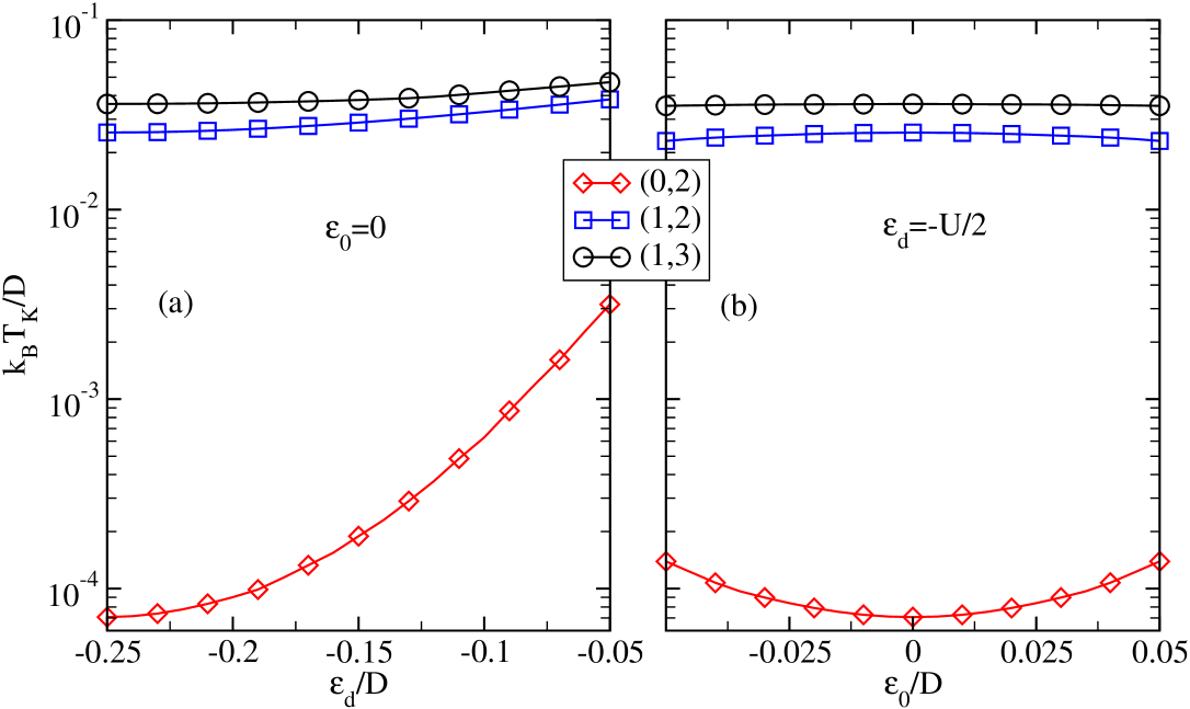
Figure 5: (Color online) Kondo temperature as function of $\varepsilon_{d}$ ($\varepsilon_{0}=0$) (a) and $\varepsilon_{0}$ ($\varepsilon_{d}=-U/2$) (b) for various configuration of $(N_{L},N_{R})$ as shown in the legend. The other parameter are the same as in the previous figures.

In conclusion, we have presented a detailed study of the Kondo temperature of a single molecule break junction. By employing a numerical renormalization group we show that $T_{K}$ is strongly dependent of the parity of the number of atomic sites in each piece of QW connecting the molecule to the contacts. More interesting, we show that the $T_{K}$ oscillates when the parity of the number of sites of the wires changes. These oscillations are interpreted in terms of the effective hybridization function $\Delta(\omega)$. For $(even,even)$ and $(odd,odd)$ configurations the effective coupling $\Delta$ is minimum and maximum, respectively, while for $(even,odd)$ or $(odd,even)$ configurations $\Delta$ possesses an intermediate value. Within this picture, the huge variation of $T_{K}$ is readily estimated by a simple analytical calculation, which can vary up to a factor of $10^{2}$ [in the case of changing from ($even,even$) to ($even,odd$)]. Our results provide a very clear picture of the main ingredient responsible for the dramatic dependence of $T_{K}$ on geometrical configuration of single molecule break junctions as well as of magnetic molecule on atomic layer surfaces. Moreover, we believe our results can be used to guide experimental realizations of high-$T_{K}$ experiments.

We would like to thank CNPq (under grant No. 493299/2010-3) and FAPEMIG (under grant No. CEX-APQ-02371-10) for financial support. We also wish to acknowledge valuable discussions with F. M. Souza.

References

- (1) A. C. Hewson, The Kondo problem to heavy fermions (Cambridge University Press, 1993)
- (2) J. Kondo, Prog. Theor. Phys., 32(1964)
- (3) D. Goldhaber-Gordon, H. Shtrikman, D. Mahalu, D. Abusch-Magder, U. Meirav, and M. A. Kastner, Nature 391, 156 (1998)
- (4) S. M. Cronenwett, T. H. Oosterkamp, and L. P. Kouwenhoven, Science 281, 540 (1998)
- (5) V. Madhavan, W. Chen, T. Jamneala, M. F. Crommie, and N. S. Wingreen, Sicence 280, 567 (1998)
- (6) H. C. Manoharan, C. P. Lutz, and D. M. Eigler, Nature 403, 512 (2000)
- (7) V. Iancu, A. Deshpande, and S.-W. Hla, Phys. Rev. Lett. 97, 266603 (Dec 2006)
- (8) L. Kouvenhoven, Science 268, 1440 (1995)
- (9) H. Jeong, A. M. Chang, and M. R. Melloch, Science 293, 2221 (2001)
- (10) A. Georges and Y. Meir, Phys. Rev. Lett. 82, 3508 (Apr 1999)
- (11) G. González, M. N. Leuenberger, and E. R. Mucciolo, Phys. Rev. B 78, 054445 (Aug 2008)
- (12) L. G. G. V. Dias da Silva, N. P. Sandler, K. Ingersent, and S. E. Ulloa, Phys. Rev. Lett. 97, 096603 (Aug 2006)
- (13) J. J. Parks, A. R. Champagne, G. R. Hutchison, S. Flores-Torres, H. D. Abruña, and D. C. Ralph, Phys. Rev. Lett. 99, 026601 (Jul 2007)
- (14) H.-S. Sim, H.-W. Lee, and K. J. Chang, Phys. Rev. Lett. 87, 096803 (Aug 2001)
- (15) Z. Liu, S.-Y. Ding, Z.-B. Chen, X. Wang, J.-H. Tian, J. R. Anema, X.-S. Zhou, D.-Y. Wu, B.-W. Mao, X. Xu, B. Ren, and Z.-Q. Tian, Nature Communications 2, 305 (2011)
- (16) N. J. Tao, Nature Nanotechnology 1, 173 (2006)
- (17) R. H. M. Smith, Y. Noat, C. Untiedt, N. D. Lang, M. C. van Hemert, and J. M. van Ruitenbeek, Nature 419, 906 (2002)
- (18) R. H. M. Smit, C. Untiedt, G. Rubio-Bollinger, R. C. Segers, and J. M. van Ruitenbeek, Phys. Rev. Lett. 91, 076805 (Aug 2003)
- (19) K. G. Wilson, Rev. Mod. Phys. 47, 773 (Oct 1975)
- (20) R. Bulla, T. A. Costi, and T. Pruschke, Rev. Mod. Phys. 80, 395 (Apr 2008)
- (21) Y.-S. Fu, S.-H. Ji, X. Chen, X.-C. Ma, R. Wu, C.-C. Wang, W.-H. Duan, X.-H. Qiu, B. Sun, P. Zhang, J.-F. Jia, and Q.-K. Xue, Phys. Rev. Lett. 99, 256601 (Dec 2007)
- (22) K. Chen and C. Jayaprakash, Phys. Rev. B 52, 14436 (Nov 1995)
- (23) All the results were obtained using the conventional NRG discretization parameter and keeping typically states at each iteration.
- (24) H. R. Krishna-murthy, J. W. Wilkins, and K. G. Wilson, Phys. Rev. B 21, 1003 (Feb 1980)
- (25) F. D. M. Haldane, Phys. Rev. Lett. 40, 416 (Feb 1978)