Magnetic moment non-conservation in magnetohydrodynamic turbulence models

Abstract

The fundamental assumptions of the adiabatic theory do not apply in presence of sharp field gradients as well as in presence of well developed magnetohydrodynamic turbulence. For this reason in such conditions the magnetic moment $\mu$ is no longer expected to be constant. This can influence particle acceleration and have considerable implications in many astrophysical problems.

Starting with the resonant interaction between ions and a single parallel propagating electromagnetic wave, we derive expressions for the magnetic moment trapping width $\Delta\mu$ (defined as the half peak-to-peak difference in the particle magnetic moment) and the bounce frequency $\omega_{b}$. We perform test-particle simulations to investigate magnetic moment behavior when resonances overlapping occurs and during the interaction of a ring-beam particle distribution with a broad-band slab spectrum.

We find that magnetic moment dynamics is strictly related to pitch angle $\alpha$ for a low level of magnetic fluctuation, $\delta B/B_{0}=(10^{-3},\,10^{-2})$, where $B_{0}$ is the constant and uniform background magnetic field. Stochasticity arises for intermediate fluctuation values and its effect on pitch angle is the isotropization of the distribution function $f(\alpha)$. This is a transient regime during which magnetic moment distribution $f(\mu)$ exhibits a characteristic one-sided long tail and starts to be influenced by the onset of spatial parallel diffusion, i.e., the variance $\langle(\Delta z)^{2}\rangle$ grows linearly in time as in normal diffusion. With strong fluctuations $f(\alpha)$ isotropizes completely, spatial diffusion sets in and $f(\mu)$ behavior is closely related to the sampling of the varying magnetic field associated with that spatial diffusion.

I Introduction

In this paper we study magnetic moment $\mu$ conservation for charged particles in presence of a single electromagnetic wave as well as in presence of turbulent magnetic fields having one dimensional spectra comparable to those measured in the solar wind. Magnetic moment conservation is an important topic in plasma physics. Indeed, some of the most commonly used theories that describe particle motion in perturbed magnetic fields are based on the assumption that particles magnetic moment is on average constant over a gyroperiod. When $\mu$ is not conserved, this approximation is not allowed and its effects can have a bearing on several astrophysical phenomena such as coronal heating, cosmic ray transport, temperature anisotropies observed in the solar wind Marsch (1991) and particle acceleration near reconnection sites Knizhnik et al. (2011). Furthermore this issue is strictly related to particle confinement in plasma machines and dynamically chaotic systems Chirikov (1987). Therefore we want to established the validity range of the adiabatic approximation and the key mechanisms that regulate magnetic moment non-conservation.

The guiding center approximation Rossi & Olbert (1970) splits particle motion into the motion of the guiding center and the gyromotion around it. When analyzing charged particle motion in nonuniform electromagnetic fields, we would like to neglect the rapid and relatively uninteresting gyromotion, focusing instead on the far slower motion of the guiding center. Averaging the particle equation of motion over the gyrophase, we obtain a reduced equation that describes the guiding center motion. In the non-relativistic case the equation of motion of the guiding center in the direction parallel to the magnetic field reads

$$\frac{dp_{\parallel}}{dt}=-\mu\nabla_{\parallel}B+qE_{\parallel},$$ (1)

where particle magnetic moment is defined as $\mu=v_{\perp}^{2}/B$ and $\nabla_{\parallel}=(\mathbf{\hat{B}}\cdot\nabla)$ is the spatial derivative along the field direction. In the perpendicular direction the guiding center drifts with the velocity

$$v_{D}=\frac{{\bf F}\times{\bf B}}{qB^{2}},$$ (2)

where ${\bf F}=[q{\bf E}-\mu\nabla B-(mv^{2}_{\parallel})\nabla_{\parallel}{\bf B}]$ is the total force acting on the guiding center, averaged over a gyroperiod, in the (non-inertial) frame co-moving with the guiding center. Therefore, as long as a particle moves through slowly varying electric and magnetic fields, its guiding center behaves like a particle with a magnetic moment $\mu$ conserved.

This approximation is valid when the smallest length-scales of the electromagnetic fields are much larger than the particles Larmor radius, i.e., when particle magnetic moment is a constant of motion on average over the particle gyroperiod. This corresponds to the well-known Born-Oppenheimer approximation in quantum mechanics. This description for particle motion in a non-uniform magnetic field is also useful for numerical simulations. Indeed direct simulations of kinetic equations (Vlasov, Boltzmann) with a large magnetic field require the numerical resolution of small spatial and time scales induced by the gyration along the magnetic field. The guiding center approximation, as well as gyrokinetics, are approximate models describing particle motion in presence of a strong magnetic field. However, the assumption that the scale of variation of the magnetic field is much larger than the particle Larmor radius can break down in presence of turbulence. Turbulent magnetic fluctuations are observed in space plasmas in practically all environments and at all scales. Furthermore the presence of waves in collisionless plasma introduces through wave-particle interactions a finite dissipation. In this case it seems invalid to resort to a guiding center theory.

When the amplitude of the magnetic fluctuations is lower than that of the mean magnetic field (averaged over the fluctuations time-scale), a perturbation approach called quasilinear approximation is applicable Jokipii (1966); Urch (1977); Jones et al. (1998). In this case the resonant fluctuations make the dominant contribution to particle scattering. The resonance condition for wave-particle interaction is given by:

$$\omega-k_{\parallel}v_{\parallel}=n\Omega$$ (3)

where $\omega$ is the wave frequency, $k_{\parallel}$ and $v_{\parallel}$ are respectively the wavevector and the particle velocity along the mean magnetic field ${\bf B}_{0}$, and $\Omega=qB/m$ is the particle gyrofrequency. Landau resonance Landau (1946) is found at $n=0$, while $n=\pm 1$, $\pm 2,\,\ldots$ are the cyclotron resonances. In linear theory these resonances are represented by delta functions. In presence of well-developed magnetohydrodynamic turbulence we expect that the discrete resonances to be significantly broadened due to the rapid decorrelation of the waves phases in strong turbulence Chandran (2000).

The particle reaction to the perturbation is always periodic except when condition (3) is satisfied. In this case the perpendicular electric force due to the wave remains in phase with the particle cyclotron motion and particle reaction is secular or resonant and, over short times, non-oscillatory. The secular electric force acting on a given particle is constant over a particle gyroperiod, so that the magnetic moment is no longer conserved.

Charged particles are scattered by their interaction with the waves and undergo pitch angle diffusion. The pitch angle, $\theta=\arctan(v_{\perp}/v_{\parallel})$, is the angle between the direction of the magnetic field and the particle’s helical trajectory. Scattering from magnetic fluctuations causes the distribution of pitch angle cosine, $\alpha=v_{\parallel}/|v|$, to become isotropic. Magnetic moment, $\mu$, is formally related to the time averages of the cosine of pitch angle by:

$$\mu\sim\frac{v^{2}_{\perp}}{|B|}=\frac{v^{2}}{|B|}(1-\alpha^{2})$$ (4)

We therefore expect the behavior of magnetic moment to be strongly related to pitch angle behavior.

II Stochastic motion, trapping width and resonance overlapping

Wave-particle interactions usually involve multiple resonances. Particle motion is substantially different depending on when these resonances overlap or not. Numerical simulations show a complex behavior that cannot be approached analytically, e.g., it is not possible to write an equation for the evolution of particles distributions when two resonances overlap Smith & Kaufman (1978). Such motions in the presence of overlapping resonances are commonly labeled stochastic.

It is important to distinguish between two different kinds of stochasticity. Wave-particle interaction in presence of of uncorrelated small amplitude electromagnetic waves or plasma turbulence is called extrinsically diffusive Lichtenberg & Wood (1989). In this case the regular phase space structure for a charged particle interacting resonantly with an electromagnetic wave is perturbed by neighboring uncorrelated waves. This leads to extrinsic stochasticity and diffusive behavior. On the other hand nonlinear systems, such as particle interacting resonantly with a large amplitude obliquely propagating (with respect to $\mathbf{B}_{0}$) electromagnetic plasma wave, can exhibit intrinsic stochasticity. Indeed, when the wave amplitude is sufficiently large, the resonances at the gyrofrequency harmonics are sufficiently broadened that they overlap with adjacent primary resonances. Therefore particles interacting even with a single monochromatic wave may exhibit intrinsically stochastic and diffusive behavior Karimabadi et al. (1990). This is the regime of nonlinear diffusion and irreversible chaotic mixing of orbits.

Because one of the main hypothesis of quasilinear theory is that particles dynamics is adequately modeled by their unperturbed trajectories, the quasilinear timescale $\tau_{c}$ must be much smaller than the timescale for the onset of nonlinear orbit effects $\tau_{nl}$ (cf. Weinstock, 1969; Davidson, 1972):

$$\tau_{c}\ll\tau_{nl}\sim\frac{1}{\omega_{b}},$$ (5)

where ${\omega_{b}}$ is the bounce frequency. This means that the turbulent spectrum should be broad enough so that the typical timescale for a charged particle to interact with a resonant wave-packet would be much less than its typical bounce time, $\tau_{b}=2\pi/\omega_{b}$, in a monochromatic wave at the characteristic wavenumber and frequency of the wave-packet. The bounce time, $\tau_{b}$, for a particle in resonance with an electromagnetic wave is proportional to its oscillation period in the pseudo-potential well governing the resonant wave-particle interaction Karimabadi et al. (1990). This interaction can be approximated by a Hamiltonian pendulum in the vicinity of the resonance point.

Particles in resonance with a single finite amplitude fluctuation undergo a finite amplitude nonlinear oscillation. This is the so-called trapping width, $\Delta v_{\parallel}$, given by the half peak-to-peak difference in the particle velocity parallel component. The trapping width and the bounce frequency for a nonrelativistic particle interacting resonantly with an electromagnetic wave are given by Equations (5a)–(5c) of Ref. Karimabadi et al. (1992). These approximate expressions for $\Delta v_{\parallel}$ and $\omega_{b}$ yield considerable physical insight into the diffusion process Mace et al. (2012) when used in conjunction with the quasilinear diffusion coefficient.

III Magnetic moment trapping width

From the trapping width, $\Delta v_{\parallel}$, and bounce frequency, $\omega_{b}$, computed by Ref. Mace et al. (2012) for the case of a circularly polarized electromagnetic wave (see Appendix), it is possible to derive the pitch angle trapping half width as:

$$\Delta\alpha=\frac{\Delta v_{\parallel}}{v}=2\left[(1-\alpha^{2})^{1/2}|\alpha|\frac{\delta B}{B_{0}}\right]^{1/2}$$ (6)

As magnetic moment $\mu$ is related to $\alpha$ by Eq. (4), we can write the trapping width for the magnetic moment as:

$$\Delta\mu=2\alpha\Delta\alpha=4\alpha\left[(1-\alpha^{2})^{1/2}|\alpha|\frac{\delta B}{B_{0}}\right]^{1/2}$$ (7)

These expressions apply to a circularly polarized wave. From Eq. (7) we expect that $\mu$ continues to be a good adiabatic invariant when resonances are not present or when particle interacts with extremely small amplitude waves.

IV Model and governing equations

We investigate magnetic moment behavior first during the resonant interaction between one ion and a circularly polarized magnetic wave, then when resonance overlapping occurs and finally during the interaction between a distribution of particles and a broad-band turbulent spectrum. Because some of our normalization quantities are expressed in terms of typical time and length scales of the turbulence slab model Jokipii (1966); Bieber et al. (1994), we first give a general summary of the slab model.

For the general one dimensional (1D) slab description, turbulence is made up of a sum of right and left handed circularly polarized nondispersive plane Alfvén waves propagating in the parallel direction. The magnetic field fluctuations are perpendicular to both the wave vector and the mean field. The fields are assumed to be magnetostatic. This amounts to the auxiliary assumption that the average particle speed is well in excess of the phase speed of the underlying linear wave mode. We ignore nonlinear wave-wave couplings in the spirit of quasilinear theory (see e.g., Kennel & Petschek, 1966; Swanson, 1989; Stix, 1992).

Arbitrary length scale	$\lambda$
Alfvén speed	$v_{A}$
Unit transit time	$\tau_{A}=\lambda/v_{A}$
Magnetic field	$B_{0}=\sqrt{4\pi\rho}\ v_{A}$
Electric field	$E_{n}=(v_{A}/c)B_{0}=v_{A}^{2}\sqrt{4\pi\rho}/c$

Table 1: Characteristic physical quantities.

Considering Alfvén waves propagating with $\omega/k=\omega/k_{\parallel}\simeq\pm v_{A}$, the magnetostatic approximation implies $|{\bf v}|\gg v_{A}$ (strictly $|v_{\parallel}|\gg v_{A}$). Since particle energy is conserved in a frame moving at the parallel component of the phase velocity of the wave ($\omega/k_{\parallel}$), quasilinear theory Kennel & Petschek (1966) implies:

$$(v_{\parallel}-\omega/k_{\parallel})^{2}+{v_{\perp}}^{2}=\mbox{const}.$$

Because of the magnetostatic assumption, particle energy is conserved, i.e., energy diffusion in forbidden and in velocity space the resonant interaction diffuses pitch angle and gyrophase only. Finally, we ignore all inter-particle correlations resulting from their mutual interaction through their microfields (e.g.,Coulomb collisions, Debye shielding, and polarization). Furthermore the feedback of the particles on the macroscopic fields is ignored, i.e., we consider only test particles in prescribed macroscopic magnetostatic fields. By virtue of the inequality $v_{\parallel}\gg v_{A}$, the turbulent electric field of the order $(\delta B/B_{0})v_{A}B_{0}$ is negligible compared to the motional electric field of the particle, $v_{\parallel}B_{0}$.

The dispersionless hypothesis rules out phase mixing and, hence, phase decorrelation due to this process. Consequently the only way for a particle to see a “wavepacket” phase-decorrelate is to traverse an autocorrelation length of the turbulence Kaiser et al. (1978). The autocorrelation time in this case is given by

$$\tau_{c}=\frac{1}{|\Delta(\omega-k_{\parallel}v_{\parallel})|}=\frac{1}{|v_{\parallel}\Delta k_{\parallel}|}\simeq\frac{\lambda_{c}}{|v_{\parallel}|},$$ (8)

where $\lambda_{c}$ is the turbulence correlation length.

The behavior of a test particle is described by its time dependent position ${\bf r}(t)$ and three-dimensional velocity ${\bf v}(t)$, that are advanced according to $d{\bf r}/dt={\bf v}$ and the Lorentz force equation:

$$m\frac{d{\bf v}}{dt}=q\left[{\bf E}+\frac{\mathbf{v}}{c}\times{\bf B}\right]$$ (9)

In order to render the equations non-dimensional, we use the characteristic quantities listed in Table 1, where $\tau_{A}$ is the Alfvén crossing time, $v_{A}$ is the Alfvén velocity, $\lambda=l_{z}$ is the turbulence coherence length related to the turbulence correlation length $\lambda_{c}$ ($\lambda_{c}=0.747l_{z}$ for our particular slab configuration Mace et al. (2000)). For the static case also the light speed may be used as a characteristic quantity Minnie et al. (2005). The introduction of an Alfvén speed in our test particle model, where the waves are treated as static, may appear rather artificial. However, the magnetostatic assumption is valid here provided that $|v_{\parallel}|\gg v_{A}$ and we introduce $v_{A}$ in anticipation of future work where we will drop the magnetostatic hypothesis.

With our choice for the characteristic quantities (Table 1) the dimensionless equations of motion of our charged test particles are given by:

$$\frac{d{\bf r}}{dt} = {\bf v}$$ (10)

$$\frac{d{\bf v}}{dt} = \beta({\bf E}+{\bf v}\times{\bf B})$$ (11)

Here $\beta=\Omega\tau_{A}$ (cf. $\alpha$ parameter in Ref. Ambrosiano et al., 1988) couples particle and field spatial and temporal scales and provides a particularly useful means to relate our numerical experiments to space and astrophysical plasmas. In general in a turbulent collisionless plasma the bandwidth of the inertial range fluctuations may extend from large fluctuations at the correlation scale, $\lambda_{c}$, to small fluctuations at the ion inertial scale. In this case $\beta\gg 1$ and the turbulent time-scales are much slower than the typical particle gyroradius Goldstein et al. (1986).

The resonant condition for the static case in terms of $\beta$ is given by

$$k_{res}\lambda=\frac{n\beta}{\alpha(v/v_{A})}=\frac{n\beta}{(v_{\parallel}/v_{A})}$$ (12)

Time is advanced through a fourth-order Runge-Kutta integration method with an adaptive time-step (pp. 708-716 of Ref. Press et al., 1992).

V Numerical simulations

Particles are loaded randomly in space at $t=0$ throughout a one-dimensional simulation box of length $L$. The fields are described in the following sections. In spherical coordinates, with the polar axis along the $z$-direction parallel to the mean magnetic field of strength $B_{0}$, particle velocity components are:

$$v_{x}=v\sin\theta\cos\phi\quad v_{y}=v\sin\theta\sin\phi\quad v_{z}=v\cos\theta$$ (13)

Particles initial velocities are randomly distributed in the gyrophase $\phi$ between $[0:2\pi]$, while the velocity magnitude $v$ and pitch angle $\theta$ are determined by the particular numerical experiment.

Typical particle velocities used in our simulations are $10v_{A}$ and $100v_{A}$, satisfying the magnetostatic constraint. In our analysis magnetic moments are expressed in units of the characteristic quantity $\mu_{n}=v^{2}/B_{0}$. We also define $\delta b=\delta B/B_{0}$.

Figure 1: Gyroresonant interaction between a circularly polarized wave and a particle with $v=100v_{A}$ and $\alpha=1/8$: cosine of pitch angle $\alpha$ (top row), particle magnetic moment $\mu$ (middle row) and parallel component of the induced electric field bottom (row). Different columns correspond to different wave amplitude: $\delta b=0.001$ (first column), $\delta b=0.01$ (second column), $\delta b=0.1$ (third column) and $\delta b=1.0$ (fourth column).

The statistic analysis of particle magnetic moment involves averaging trajectories over the particle gyroperiod $\tau_{g}=2\pi/\Omega$. For each simulation we compute the effective number of gyroperiods $N_{\tau_{g}}$ that particles complete in a given magnetic field configuration as:

$$N_{\tau_{g}}=\int_{0}^{t}\frac{dt}{2\pi}\frac{eB(t)}{mc}.$$ (14)

where $B(t)$ is the intensity of the total magnetic field. When $\delta b\ll 1$, $B(t)\simeq B_{0}$; however increasing $\delta b$ toward unity the waves contribution to the strength of the total magnetic field $B(t)$ is not negligible.

V.1 Single wave

We start studying the ion motion in presence of a constant magnetic field ${\bf B}_{0}$ and a perpendicular left-handed circularly polarized wave with

$${\bf B}=\delta B_{x}\cos(k_{0}z)\,\mathbf{\hat{e}}_{x}-\delta B_{y}\sin{(k_{0}z)}\,\mathbf{\hat{e}}_{y}+B_{0}\,\mathbf{\hat{e}}_{z},$$ (15)

where $\delta B_{x}$ and $\delta B_{y}$ are the amplitudes of the wave and $k_{0}$ is the wavevector. We assume $\delta B_{x}=\delta B_{y}=\delta B$ for the rms average values. In these simulations $\beta=10^{3}$, $v=100v_{A}$ and $\alpha=0.125$ ($\theta=82^{\circ}$).

We follow the test-particles until they complete $N_{\tau_{g}}=100$ gyroperiods. For the resonance condition, Eq. (12), we set $k_{0}=80/\lambda$. Particles injected with a pitch angle cosine different to $\alpha=0.125$ will not be in resonance with this wave, exhibiting a different behavior. For a direct comparison we also inject non-resonant particles, i.e., with $\alpha=0.5$ ($\theta=60^{\circ}$).

Figure 1 shows the time evolution of the cosine of pitch angle $\alpha$, particle magnetic moment $\mu$, and the parallel component of the induced electric field $E_{z}$, for a resonant particle ($\alpha=0.125$). Different columns corresponds to different values of the wave amplitude: $\delta b=0.001$ (first column), $\delta b=0.01$ (second column), $\delta b=0.1$ (third column) and $\delta b=1.0$ (fourth column).

When the parallel component of the induced electric field is almost constant and equal to $E_{z}\sim-v_{\perp}\delta b$, the resonant interaction produces variations that are secular over a gyroperiod. However an oscillation occurs over a longer time, the bounce period $\tau_{b}=2\pi/\omega_{b}$ (where $\omega_{b}$ is the bounce frequency discussed in Section II). This is the typical timescale over which the velocity, and hence the particle trajectory, exhibits significant deviations from the linear $v_{\parallel}=\text{const}$ and $v_{\perp}=\text{const}$ case.

$\delta b$	$\Delta\alpha_{th}$	$\Delta\alpha_{sim}$	$\Delta\mu_{th}$	$\Delta\mu_{sim}$
$0.001$	$0.022$	$0.02$	$0.0056$	$0.0055$
$0.01$	$0.07$	$0.075$	$0.0176$	$0.02$
$0.1$	$0.2227$	$0.2$	$0.0556$	$0.055$
$1.0$	$0.704$	$0.6$	$0.176$	$0.175$

Table 2: Trapping width values for $\alpha$ and $\mu$: comparison between theoretical (subscript th) and numerical (subscript sim) values.

In Section III we derived the analytical expression for the half trapping-width of magnetic moment for a particle interacting with a left or right handed circularly polarized wave (see Eq. 7). We now compute the values of the half peak-to-peak difference in $\alpha$ and $\mu$, $\Delta\alpha=(\alpha_{max}-\alpha_{min})/2$ and $\Delta\mu=(\mu_{max}-\mu_{min})/2$, for the resonant interaction simulations. These values and those obtained from the theoretical expressions (6)-(7) are listed in Table 2 and are in good agreement, confirming the validity of equations (6)-(7) and reinforcing the intuitively idea that magnetic moment and pitch angle behaviors are strictly related.

To compare resonant and non-resonant dynamics, we show in Figure 2 the time evolution of cosine of pitch angle $\alpha$ (first row), magnetic moment $\mu$ (third row), and their distribution functions $f(\alpha)$ (second row) and $f(\mu)$ (fourth row) at the end of the simulation, for a resonant particle with $\alpha=0.125$ (left column), and a non-resonant one with $\alpha=0.5$ (right column). In contrast with the resonant case in which $\alpha$ and $\mu$ exhibit well-known secular variations with typical period equal to $\tau_{b}$, the $\alpha$ and $\mu$ profiles for a non-resonant particle show a regular oscillating behavior, a distinctive signature of regular particle motion. The values of the half peak-to-peak difference in $\alpha$ and $\mu$ obtained from the simulation are $\Delta\alpha_{sim}=0.0025$ and $\Delta\mu_{sim}=0.003$. These are smaller than the theoretical values computed from equations (6)-(7) with $\delta b=0.01$ and $\alpha=0.5$, for which we obtain $\Delta\alpha_{th}=0.1316$ and $\Delta\mu_{th}=0.1316$.

The distribution functions $f(\alpha)$ and $f(\mu)$ (Figure 2) for a resonant particle are more spread in $\alpha$ and $\mu$ and are centered around their initial values $\alpha=0.125$ and $\mu=0.98$. In the non-resonant case, $f(\mu)$ remains peaked at its initial value, i.e., its magnetic moment is constant during particle motion. The spread in $\alpha$ of its distribution is $\sim 10\%$, small compared to the resonant case spreading of $\sim 40\%$.

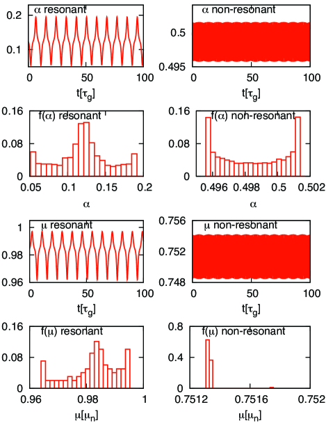
Figure 2: Time evolution of cosine of pitch angle $\alpha$ (first row) and its distribution function $f(\alpha)$ (second row), time evolution of magnetic moment $\mu$ (third row) and its distribution function $f(\mu)$ (fourth row) of resonant ($\alpha=0.125$, left column) and non-resonant particle ($\alpha=0.5$, right column). $v=100\,v_{A}$.

Figure 3 shows the distribution functions, $f(\alpha)$ and $f(\mu)$, at the end of the simulation for $1000$ resonant and non-resonant particles injected in the simulation box with random positions and phases. For non-resonant particles (right column) the distributions remain peaked around their initial values $\alpha=0.5$ and $\mu/\mu_{n}=0.75$ with very little spreading. For the resonant particles (left column) $f(\alpha)$ acquires a Gaussian shape centered around its initial value $\alpha=0.125$. Furthermore it spreads of $\sim 0.1$, comparable to the trapping width for the single particle $2\Delta\alpha=0.014$ (Figure 2). The magnetic moment distribution for the resonant case has a characteristic shape found for $\mu$ in the parameter range in which pitch angle exhibits a Gaussian distribution and the density distribution function is still isotropic (particle free-streaming regime). As for the pitch angle, the spread in the magnetic moment distribution of $\sim 0.03$ is comparable to the trapping width for the single particle $2\Delta\mu=0.00352$ (see Eq. 7 and Figure 2).

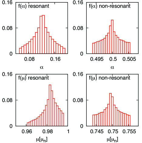
Figure 3: $f(\alpha)$ (first row) and $f(\mu)$ (second row) at the end of the simulation for an initial distribution of $1000$ resonant (left column) and non-resonant (right column) particles randomly distributed in the simulation box. $\delta b=0.01$.

V.2 Overlapping resonances

In order to understand the effect of overlapping resonances on particle magnetic moment, we perform a numerical experiment with four different particles in the simulation box with random initial positions, same initial velocity $v=100\,v_{A}$, but different values for pitch angle cosine: $\alpha_{1}=1/2,\alpha_{2}=1/4,\alpha_{3}=1/8,\alpha_{4}=1/32$. For $\beta=10^{3}$, making use of the resonance condition for the static case [Eq. (12)], the cyclotron resonances $n=1$ for the different values of $\alpha$ are expected for $k_{1}\lambda=20$, $k_{2}\lambda=40$, $k_{3}\lambda=80$, and $k_{4}\lambda=320$.

The total magnetic field is given by:

$${\bf B}=B_{0}{\bf\hat{e}}_{z}+\sum_{i=1}^{4}\delta b\cos[k_{i}z+\phi_{i}]{\bf\hat{e}}_{x}-\sum_{i=1}^{4}\delta b\sin[k_{i}z+\phi_{i}]{\bf\hat{e}}_{y},$$ (16)

where the $\phi_{i}$ are random phases. Taking into account resonance broadening effects, all particles with parallel velocities in the range

$$v_{\parallel}-\Delta v_{\parallel}<v_{\parallel}<v_{\parallel}+\Delta v_{\parallel}$$ (17)

can potentially resonate with a wave, whose wave number is $k_{\parallel}=\Omega/v_{\parallel}$. As found by Ref. Chirikov (1978), the direct evidence of resonances overlapping is the disappearance of constants of motion, i.e., the onset of stochasticity in the Hamiltonian formalism. We make simulations with four different waves amplitudes $\delta b$ = 0.001, 0.01, 0.1, and 1.0. The values of the trapping half-widths $\Delta v_{\parallel}$ computed for the different pitch angles with Eq. (A) are listed in Table 3 for the different $\delta b$ considered.

$\delta b$	$\alpha=1/2$	$\alpha=1/4$	$\alpha=1/8$	$\alpha=1/32$
$0.001$	$4.16$	$3.1$	$2.227$	$1.3$
$0.01$	$13.1$	$9.85$	$7.042$	$3.583$
$0.1$	$41$	$31.1$	$22.27$	$11.33$
$1.0$	$131$	$98.3$	$70.42$	$35.83$

Table 3: Values of $\Delta v_{\parallel}$ for $\alpha$ =1/2,  1/4,  1/8,  and 1/32 resonances at different $\delta b$.

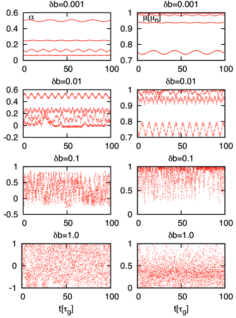
Figure 4: Transition from non-overlapping to overlapping resonances: $\alpha$ (left column) and $\mu$ (right column) profiles varying the waves amplitude: $\delta b=0.001$ (first row), $\delta b=0.01$ (second row), $\delta b=0.1$ (third row), $\delta b=1.0$ (fourth row).

Figure 4 shows time histories of pitch angle cosine $\alpha$ (left column) and magnetic moment $\mu$ (right column) profiles for various $\delta b$. Again similar behavior is seen for $\alpha$ and $\mu$. For the smallest wave amplitude, $\delta b=0.001$, it is possible to recognize very well the four different resonances in the profiles of $\alpha$ and $\mu$. For $\delta b=0.01$ the resonance at $\alpha_{3}=1/8$ is overlapping with the resonance at $\alpha_{4}=1/32$. Indeed, the initial parallel velocity of the particle injected at the smallest pitch angle, $v_{\parallel,4}=3.125v_{A}$, lies in the range of velocities [see Eq. (17)] in possible resonance with $k_{\parallel}=k_{3}$. For higher wave amplitudes, $\delta b=0.1$ and $\delta b=1.0$, the condition (17) is satisfied by all particles velocities. Stochasticity arises and the different resonances are indistinguishable.

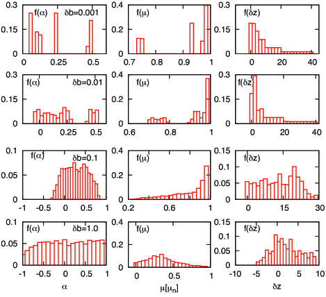
Figure 5: Transition from non-overlapping to overlapping resonances with varying wave amplitude: $\delta b=0.001$ (first row), $\delta b=0.01$ (second row), $\delta b=0.1$ (third row), $\delta b=1.0$ (fourth row). The distribution functions $f(\alpha)$ (left column), $f(\mu)$ (central column) and $f(\delta z)$ (right column) are averaged over time.

The distribution functions $f(\alpha)$, $f(\mu)$ and $f(\delta z)$ (where $\delta z=z-z_{0}$ is the displacement along $z$ relative to the particle initial position $z_{0}$) after $100\tau_{g}$ (Figure 5) exhibit similar characteristics.

For $\delta b=0.001$, $f(\alpha)$ and $f(\mu)$ are peaked in correspondence of their four initial values because of the good resonances separation. $f(\delta z)$ shows that the particles are simply free-streaming in the parallel direction and, depending on their initial parallel velocity, they cover shorter or longer distances along $z$.

For $\delta b=0.01$, $f(\alpha)$ spreads around its initial four peaks because particle interact resonantly with waves of larger amplitude, and resonances overlap for $\alpha<1/4$, as discussed previously. Similar effects are shown also by $f(\mu)$, confirming that for small $\delta b$ the resonant interaction affects magnetic moment and pitch angle in similar ways.

While for $\delta b=0.01$ particles continue to free-stream in the z-direction, different profiles for $f(\delta z)$ appear for $\delta b=0.1$. Pitch angle distribution begins to isotropize and magnetic moment exhibits a one-sided long tail distribution extending toward smaller $\mu$. This behavior is similar to the regime found previously in the single wave experiment when $f(\alpha)$ is nearly isotropic, $f(\delta z)$ still indicates particles free-streaming, and the magnetic moment distribution displays a long tail.

For $\delta b=1.0$, by $t=100\tau_{g}$ the pitch angle cosine distribution $f(\alpha)$ has become completely isotropic, while $f(\delta z)$ approaches a gaussian distribution indicative of spatial diffusion. In this regime $f(\mu)$ loses its long-tail and starts to acquire a gaussian shape. In that way we have identified three distinct regimes of statistical magnetic moment behavior with increasing degree of turbulence.

VI Slab spectrum

In this section we present the results of our numerical simulations of test-particles in presence of a broad-band slab spectrum [see Eq. (19) and Figure 6]. We have performed simulations for different particles velocities and amplitude of the magnetic field fluctuations.

Simulations use a unidimensional computational box of length $L=10000\,l_{z}$ ($l_{z}=1$ is the coherence scale for the slab spectrum) with $N_{z}=2^{28}=268,435,456$ grid points. The magnetic field in physical space is generated from a spectrum $P(k)$ in Fourier space, via inverse fast Fourier transform (FFT). The turbulent magnetic field is given by:

$${\bf B}(z)=B_{0}{\bf e}_{z}+\delta{\bf B}(z),$$ (18)

with $\delta{\bf B}(z)=\delta B_{x}(z)\,{\bf\hat{e}}_{x}+\delta B_{y}(z)\,{\bf\hat{e}}_{y}$ and the solenoidality condition is identically satisfied.

The modes of the magnetic field components in k-space are given by:

$$\delta B_{x}(k_{n})=[P(k_{n})]^{1/2}e^{i\Phi_{n}}$$

$$\delta B_{y}(k_{n})=[P(k_{n})]^{1/2}e^{i\Psi_{n}}$$

where $k_{n}=2\pi n/L$ and $\Phi_{n}$ and $\Psi_{n}$ are random phases. The slab spectrum $P(k)$ is given by:

$$P(k_{n})=\begin{cases}C_{slab}[1+(k_{n}l_{z})^{2}]^{-5/6},&\text{for $k_{n}<k_{diss}$}\\ C_{diss}\left(\frac{k_{n}}{k_{diss}}\right)^{-7/3},&\text{for $k_{n}\geq k_{diss}$}\end{cases}$$ (19)

where $C_{slab}=2\lambda_{c}\delta b^{2}_{x,slab}$ is a constant specific to this form of the slab model, $\delta b^{2}_{x,slab}$ is the mean square fluctuation, $k_{diss}$ is the dissipation range wavenumber, $C_{diss}=C_{slab}[1+(k_{diss}l_{z})^{2}]^{-5/6}$ is the constant for the dissipation range (set by the continuity of the spectrum $P(k)$ at $k_{diss}$). The vectors of Fourier coefficients are zero-padded for $N_{max}+1\leq n\leq N_{z}$ providing an extra level of smoothness to the fields by an effective trigonometric interpolation. In all the simulations we use $N_{max}=6.7\times 10^{7}$ and a simple linear interpolation to compute the fields at the test particle position.

The resulting spectrum is shown in Figure 6.

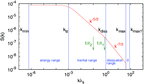
Figure 6: Power spectrum of the turbulent magnetic. $k$ is normalized to the coherence length $l_{z}$.

Several important scales are present in the system. They are labeled as $k_{min}$, $k_{l_{z}}$, $k_{diss}$, $k_{max}$ and $k_{N_{z}}$. The discrete wavenumbers are obtained through $k_{n}=2\pi n/L$ as:

$$N_{k}=\frac{L}{2\pi}k\sim 1600\,k.$$ (20)

Table 4: Characteristic scales in the spectrum.

Wavenumber index	Wavenumber value
$N_{kmin}=1$	$k_{min}=6.28\times 10^{-4}$
$N_{kl_{z}}=10^{4}$	$k_{l_{z}}=2\pi$
$N_{k_{diss}}=1.6\times 10^{6}$	$k_{diss}=10^{3}$
$N_{k_{MAX}}=6.7\times 10^{7}$	$k_{MAX}=4.2\times 10^{4}$
$N_{k_{MAX1}}=1.3\times 10^{8}$	$k_{MAX1}=8.4\times 10^{4}$

We summarize the values for $k$ and $N_{k}$ used in our simulations in Table 4, where:

• $k_{min}=2\pi/L$ is the minimum wave vector of the spectrum, corresponding to $N_{k}=N_{kmin}=1$.

• $k_{l_{z}}=2\pi/l_{z}=2\pi$ is the wave vector that marks the beginning of the inertial range. Three decades of energy containing range from $k_{min}$ to $k_{l_{z}}$ ensure turbulence homogeneity. $l_{z}$ or $\lambda_{c}=0.747l_{z}$ (see Ref. Mace et al., 2000) correspond to the typical lengths scales over which the particles attain diffusive behavior of the pitch angle. Three decades of inertial range with $P(k)\propto k^{-5/3}$ well represent solar wind conditions.

• $k_{diss}$ is the wave vector corresponding to the beginning of the dissipation range. In our model, the spectrum extends beyond $k_{diss}$ with $P(k)\propto k^{-7/3}$.

• At two decades higher wavenumber, $k_{MAX}=\sqrt{m_{i}/m_{e}}k_{diss}$ determines the end of the dissipation range.

• Extending for two decades beyond $k_{MAX}=4.2\times 10^{4}$, the spectrum includes zero-padding up to $k_{MAX1}=8.4\times 10^{4}$.

• Another important scale, not labeled in Figure 6 because it depends on test-particle velocity, is the wave vector corresponding to $z_{max}=vT_{tot}$, the distance covered by a charged test particle moving at speed $v$ in the simulation running time $T_{tot}$. To avoid periodicity effects it is important that the box length $L$ is large enough so that particles trajectories are limited to a small fraction of the full length, i.e., $L\gg z_{max}$ or $k_{min}\ll 1/z_{max}$. Periodicity might indeed give rise to artificial field lines diffusion.

We fix the value of the $\beta$ parameter equal to $10^{4}$. This corresponds approximately to observed solar wind turbulence properties at $1$ AU, as follows:

$$\beta=\Omega\tau_{A}=\left(\frac{q}{m}\right)\frac{\lambda_{c}\sqrt{4\pi\rho}}{c}=\frac{\omega_{pi}\lambda_{c}}{c}=\frac{\lambda_{c}}{\lambda_{ii}},$$ (21)

where $\lambda_{c}$ is the turbulence correlation length $\omega_{pi}=(4\pi n_{0i}{q_{i}}^{2}/m_{i})^{1/2}$ is the ion plasma frequency ($q_{i}$ and $m_{i}$ are respectively the ion charge and mass) and $\lambda_{ii}=c/\omega_{pi}=\left(c^{2}m_{i}/4\pi n_{i}e^{2}\right)^{1/2}$ is the ion inertial length. For $n_{i}=n_{e}$ then $\lambda_{ii}=(m_{i}/m_{e})^{1/2}\rho_{ie}$. Because the solar wind density at 1 AU is approximately $n\sim(1,10)\,cm^{-3}$ on average $\lambda_{ii}\sim 1000\,km$. At the same distance the turbulence correlation length $\lambda_{c}$ is approximately $10^{6}$ km Matthaeus et al. (1986) and $\beta\simeq 10^{4}$.

Typically $1000$ particles are injected in the simulation with initial random positions. Particles are loaded from a cold ring beam [see equations (13)] distribution with constant velocity magnitude, $\sin\theta$ is set equal to $(1-\alpha_{0}^{2})^{1/2}$, where $\alpha_{0}$ is the initial pitch angle cosine respect to the background field $B_{0}$. The initial gyrophase $\phi$ is chosen randomly. For all the simulations $\alpha_{0}=0.125$ ($\theta\simeq 82^{\circ}$).

Table 5: Typical values used in the simulations.

$V[v_{A}]$	$r_{L}[l_{z}]$	$k_{res}$	$\epsilon$	$t_{c}[\tau_{A}]$
$10$	$10^{-3}$	$8\times 10^{3}$	$1.33\times 10^{-3}$	$0.0747$
$100$	$10^{-2}$	$8\times 10^{2}$	$1.33\times 10^{-2}$	$0.00747$

From the previous section, we know that the behavior of magnetic moment is correlated to pitch angle behavior for a low level of magnetic fluctuation ($\delta b=0.001,0.01$). Pitch angle and magnetic moment exhibit Gaussian distribution functions typical of normal diffusion processes. Increasing the turbulence level, pitch angle distribution approaches isotropization and a transient regime is observed with the magnetic moment starting to be influenced by the onset of spatial parallel diffusion. When $f(\alpha)$ completely isotropizes, spatial diffusion sets in and $f(\mu)$ behavior is closely related to the sampling of the varying magnetic field strength associated with that spatial diffusion.

From quasilinear theory we know that velocity and real space diffusion occur at two different time scales. Typically, velocity space diffusion takes place with the time scale $\tau_{c}=\lambda_{c}/v$ shorter than the typical time scale at which parallel diffusion occurs $\tau_{\parallel}=\lambda_{\parallel}/v$, where $\lambda_{\parallel}=3D_{\parallel}/v$ is the parallel mean free path. For this reason we follow test particles in the simulation box for a time $T>\tau_{c}$, typically with $T=20\tau_{c}$. Particles parameters used in the simulations are listed in Table 5.

An important parameter in the description of energetic test particles is $\epsilon=r_{L}/\lambda_{c}$, which is sometimes called the dimensionless particle rigidity. It can be related to the bend-over wavenumber of the turbulence, $k_{bo}=1/\lambda_{c}$, and the minimum resonant wavenumber, $k^{r}_{min}=1/r_{L}$, as $\epsilon=k_{bo}/k^{r}_{min}$. For example when $r_{L}\gg\lambda_{c}$ particles experience all possible $k$-modes in few gyroperiods resonating with the energy containing scale ($k^{r}_{min}\ll k_{bo}$). For lower energies the test particles resonate in the inertial range. Those with $v=10\,v_{A}$ will resonate at the end of the inertial range ($1/r_{1}$ in Fig. 6), while those with $v\,=100v_{A}$ at the middle of the inertial range ($1/r_{2}$ in Fig. 6). Furthermore, as explained previously, the condition $k_{min}\ll z_{max}$ is necessary to avoid artificial effects in particle transport associated with periodicity of the magnetic field.

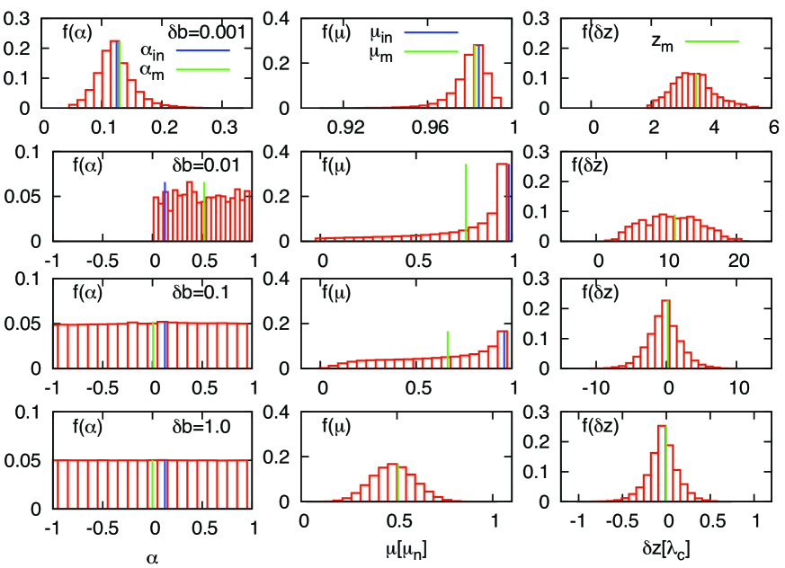
Figure 7: Distribution functions of cosine of pitch angle $f(\alpha)$ (left column), magnetic moment $f(\mu)$ (central column) and particle displacements relative to the initial position $f(\delta z)$ (right column) at $20\,\tau_{c}$ for different waves amplitude: $\delta b=0.001$ (first row), $\delta b=0.01$ (second row), $\delta b=0.1$ (third row) and $\delta b=1.0$ (fourth row). Particle parameters at injection: $v=10\,v_{A}$ and $\alpha_{0}=0.125$.

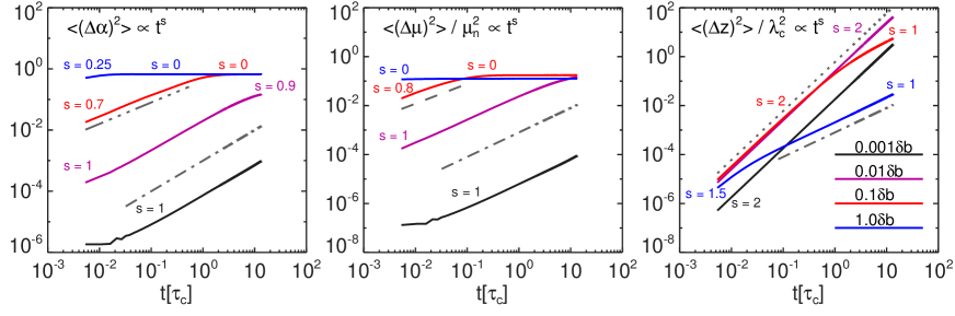
Figure 8: Statistics for $v=10\,v_{A}$. Variances for cosine of pitch angle $\alpha$ (left plot), magnetic moment $\mu$ (center plot) and particle displacements relative to the initial position $\delta z$ (right plot) at different values of $\delta b$: $\delta b=0.001$ (black line), $\delta b=0.01$ (purple line), $\delta b=0.1$ (red line) and $\delta b=1.0$ (blue line). The $s$ values indicate the different slopes for the scalings $\langle(\Delta\alpha)^{2}\rangle,\langle(\Delta\mu)^{2}\rangle$ and $\langle(\Delta z)^{2}\rangle\propto t^{s}$. The variances are fitted with the gray lines: dotted line is $s=2$, dotted-dashed line $s=1$, dashed line $s=0.8$, three dotted-dashed line $s=0.7$.

Figure 7 shows $f(\alpha)$ (left column), $f(\mu)$ (central column) and $f(\delta z)$ (right column) for a distribution of particles moving with an initial velocity $v=10\,v_{A}$ in presence of the slab spectrum [Eq. (19), Figure 6]. All the distribution functions are computed at the end of the simulation, i.e., after $20\,\tau_{c}$. The blue line and the green line indicate the initial value and the mean value of each distribution. As particles are injected at different positions, it is convenient to define the quantity $\delta z=z(j)-z(0)$ ($j$ is a temporal index). In this way it is possible to take out from the distribution function $f(\delta z)$ both the drift effect ($v_{D}t$) and particle diffusion relative to their own positions ($\Delta z_{i}$). The general expression for the $z$ position of the $i$-th particle is given by

$$z_{i}=z_{i}(0)+v_{D}t+\Delta z_{i}=z_{i}(0)+\delta z_{i}.$$ (22)

The primary diagnostic for studying particle diffusion is the variance $\sigma^{2}(t)\propto t^{s}$ of particles cosine of pitch angle, magnetic moment and position parallel to the mean field direction. Figure 8 illustrates the time evolution of the variances, $\langle\left(\Delta\alpha\right)^{2}\rangle$ (left figure), $\langle\left(\Delta\mu\right)^{2}\rangle$ (central figure) and $\langle\left(\Delta z\right)^{2}\rangle$ (left figure) for a particles distribution moving with initial velocity equal to $10\,v_{A}$. Different colors correspond to different $\delta b$ values: $\delta b=0.001$ black line, $\delta b=0.01$ purple line, $\delta b=0.1$ red line and $\delta b=1.0$ blue line. The variances are fitted with the gray lines: the dotted line is used for $s=2$, the dotted-dashed line for $s=1$, the dashed line for $s=0.8$ and the three dotted-dashed line for $s=0.7$.

For $\delta b=0.001$, $\alpha$ and $\mu$ display Gaussian distributions while particles free-stream in the $z$-direction. Particles that cover greater distance in $z$ are more scattered in pitch angle and consequently in $\mu$. Figure 8 shows superdiffusive behavior (black line, $s=2$) with particles free streaming along $z$, and later, variance characteristic of normal diffusion with $\langle\left(\Delta\alpha\right)^{2}\rangle$ and $\langle\left(\Delta\mu\right)^{2}\rangle$ scaling $\propto t$.

For $\delta b=0.01$, particles cover only one side of the $\alpha$ hemisphere continuing to travel along $z$ (purple line in Figure 8). This is the transient regime already observed in Figure 5 when $f(\mu)$ exhibits a one-sided long tail distribution toward smaller $\mu$.

For $\delta b=0.1$, pitch angle distribution becomes completely isotropic and spatial diffusion sets in, as shown by the slope $s=1$ of $\langle\left(\Delta z\right)^{2}\rangle$ in Figure 8 (red line) at the end of the simulation. The deviation from purely free-streaming or ballistic behavior means that, while the system has not become fully diffusive along the mean field direction, there are signs that diffusive processes in velocity space are beginning to diminish the free-streaming. Although $f(\mu)$ still exhibits a long-tail, the influence of spatial diffusion starts to appear. The well-pronounced peak observed in $f(\mu)$ for $\delta b=0.01$ is substantially reduced and the mean value of magnetic moment decreases. Moreover $\mu$ displays subdiffusive behavior up to $0.02\tau_{c}$. After this time particles diffuse in space and $\langle\left(\Delta\mu\right)^{2}\rangle$ attains a plateau. The Gaussian shape is not reached yet probably because spatial diffusion is just at the beginning.

For $\delta b=0.5$ [see Figure (9)] and $\delta b=1.0$, $f(\alpha)$ is isotropic, particle motion is completely diffusive in real space [as the slope $s=1$ in $\langle\left(\Delta z\right)^{2}\rangle$ in Figure 8 (blue line) shows], and $f(\mu)$ behavior is closely related to the sampling of varying magnetic field strength associated with that spatial diffusion, displaying a Gaussian distribution centered at the middle of $\mu$-space.

From a more detailed analysis of the case $\delta b=0.5$ [Figure (9)] we notice that magnetic moment variance (first figure) scales according to $\langle\left(\Delta\mu\right)^{2}\rangle\propto t^{0.17}$ (red-dashed line) up to $0.002\tau_{c}$ and after $0.005\tau_{c}$ a plateau is attained (blue-dashed line). Instead particles motion (see time evolution of $\langle\left(\Delta z\right)^{2}\rangle$, second plot) becomes fully diffusive (blue-dashed line) only after $0.007\tau_{c}$. Magnetic moment distribution $f(\mu)$ in the first part of the evolution (third plot) is in the transient regime characterized by the long tail. In contrast, when particles diffuse in real space (fourth plot), $f(\mu)$ reacquires the gaussian profile. Thus the final stage of magnetic moment variance evolution, i.e. the formation of the plateau, can be considered as a precursor for the onset of the parallel diffusion of particles in space. Of course this effect is present in pitch angle variance too, but in addition in $\mu$ behavior we have a direct signature of the onset of the spatial diffusion, that is the reappearance of the gaussian shape in the distribution function, while pitch angle distribution remains completely isotropic.

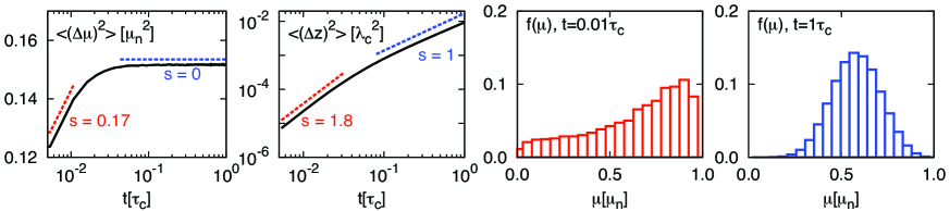
Figure 9: Statistics for $v=10\,v_{A}$ and $\delta b=0.5$. Magnetic moment variance $\langle\left(\Delta\mu\right)^{2}\rangle$ (first plot) and mean square displacement $\langle\left(\Delta z\right)^{2}\rangle$ (second plot) versus time and magnetic moment distribution function $f(\mu)$ after $0.01\,\tau_{c}$ (third plot) and at the end of the simulation (fourth plot). The $s$ values indicate the different slopes for the scaling of the variances $\langle(\Delta\mu)^{2}\rangle$ and $\langle(\Delta z)^{2}\rangle\propto t^{s}$. The variances are fitted with the dashed lines.

Thus these transitions in magnetic moment behavior are related not just to the variation of the turbulence level, but also to the different time scale at which magnetic moment conservation is studied.

The magnetic moment distribution functions $f(\mu)$ and variances $\langle\left(\Delta\mu\right)^{2}\rangle$ in the case $v=100\,v_{A}$ (not shown) exhibit the same features observed for $v=10v_{A}$. However, increasing particle speed the total number of gyroperiods, $N_{\tau_{g}}$, performed by each particle decreases; as a consequence, faster particles sample less variation in magnetic field strength. This leads to a slower spatial diffusion, i.e., for $100v_{A}$ spatial diffusion occurs on a time scale longer than $20\tau_{c}$.

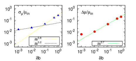
Figure 10: Standard deviation (blue triangle) and variation in magnetic moment (red circle) versus $\delta b$ for at $20\tau_{c}$ $v=100v_{A}$ and $\alpha=0.125$.

For $v=100v_{A}$ we show in Figure (10) magnetic moment standard deviation $\sigma_{\mu}/\mu_{min}$ (blue triangle) and the changes in its mean $\Delta\mu/\mu_{in}=(\bar{\mu}-\mu_{in})/\mu_{in}$ versus $\delta b$ after $20\tau_{c}$. As $\delta b$ increases toward unity the changes in magnetic moment distribution start to increase faster.

VII Conclusions

In this paper we have investigated the conservation of charged particle magnetic moment in presence of turbulent magnetic fields. For slow spatial and temporal variations of the magnetic field respect to the particle gyroradius and gyroperiod, the magnetic moment $\mu$ is an adiabatic invariant of the particle motion. Non-conservation of magnetic moment can influence particle acceleration and have considerable implications in many astrophysical problems such as coronal heating, cosmic rays transport and temperature anisotropies in the solar wind. These applications motivate the present basic study of the degree to which magnetic moments are conserved in increasingly complex models of one dimensional spectra. While all the models considered here have been very oversimplified relative to the spectra observed for example in the solar wind Bieber et al. (1994, 1996) or in simulations of MHD turbulence Oughton et al. (1994); Lehe et al. (2009), the present study is intended to contribute to the basic understanding of the conditions for the onset of magnetic moment nonconservation. We point the interested reader also to a recent study by Ref. Lehe et al. (2009) that addresses this issue from a somewhat different perspective.

In order to reproduce and extend some of the result obtained by Ref. Karimabadi et al. (1992), we started to study the resonant interaction between ions and a single parallel propagating electromagnetic wave (see Section V.1). Using the specialized expression for the trapping width $\Delta v_{\parallel}$ found by Ref. Mace et al. (2012) in the case of a single circularly polarized wave, we have been able to write a similar expression for magnetic moment (see Eq. 7). In presence of a single finite amplitude fluctuation the magnetic moment of a resonant particle undergoes a finite amplitude nonlinear oscillation too. We have performed several simulations changing both particle velocity and the amplitude of the wave. For each of them we compare the values of $\Delta\mu$ and $\Delta v_{\parallel}$ with those obtained using our specialized expression and they are in good agreement.

We designed a particular experiment to study the effects of resonances overlapping (see Section V.2). From the analysis of the distribution functions of particles pitch angle, $f(\alpha)$, magnetic moment, $f(\mu)$, and $z$-position, $f(z)$, we distinguish three different regimes. First, for a low level of magnetic fluctuation, i.e., $\delta B/B_{0}=0.001,0.01$, the magnetic moment distribution half-width is directly related to pitch angle distribution. Second for $\delta B/B_{0}=0.1$ stochasticity arises as a consequence of overlapping resonances and its effect on pitch angle is isotropization of the distribution function. This is a transient regime during which magnetic moment exhibits a one-sided long-tail distribution and starts to be influenced by the onset of spatial parallel diffusion. Finally, when $f(\alpha)$ completely isotropizes spatial diffusion sets in ( $\delta B/B_{0}=0.1$), $f(\mu)$ behavior is closely related to the sampling of varying magnetic field strength associated with that spatial diffusion.

Other studies regarding particles interaction with two electromagnetic waves as well as a flat turbulent spectrum (not shown) were also conducted and they confirmed this general picture.

Motivated by these results we studied the behavior of many particles interacting with a broad-band slab spectrum, generated in order to mimic some of the major features of the solar wind (see Figure 6): (a) three decades of the energy containing scale ensure turbulence homogeneity, (b) three decades of inertial range well-reproduce the observations and (c) two decades of dissipation range enable us to cross the “$\alpha_{min}$ barrier” related with the “resonance gap” predicted by quasilinear theory Kaiser et al. (1973, 1978). After that there are almost other two decades of zero-padding, important for the trigonometric interpolations and for the smoothness of the field. This is implemented using a numerical grid with $N_{z}=2^{28}=268,435,456$ points corresponding to $134,217,728$ wavevectors for the spectrum. Apart from the obvious limitation that this spectrum is purely one dimensional, it is constructed to correspond roughly to features of solar wind spectra observed by single spacecraft, where the fully three dimensional spectrum is in effect reduced to a one dimensional form. Information is lost in the process (see, e.g., Bieber et al., 1996).

In order to gain insight on magnetic moment conservation we have performed simulations changing both particles velocity, $v=(10,100)\,v_{A}$, and the amplitude of magnetic field fluctuations $\delta B/B_{0}=(0.001,0.01,0.1,0.5,1.0)$. Particles injected at different velocities start to resonate at different points of the spectrum. We analyzed the distribution function [see Figure 7] and the variance [see Figure (8)] of pitch angle cosine $\alpha$, magnetic moment $\mu$ and parallel position $z$.

From the experiment of resonances overlapping we know that the three different regimes of $\mu$ statistical behavior are related with other two effects: diffusion in velocity space and spatial parallel diffusion. These take place at different characteristic times, $\tau_{c}$ and $\tau_{\parallel}$ respectively. In order to investigate the effects of both processes on magnetic moment distributions, we followed test-particles in the simulation box for times $T>\tau_{c}$.

For a low level of magnetic fluctuations particles free-stream in the $z$-direction while $\alpha$ and $\mu$ exhibit gaussian distributions around their initial values. For $\delta B/B_{0}=0.01$ particles cover completely one side of the $\alpha$ hemisphere continuing to stream freely along $z$. This is the transient regime during which $f(\mu)$ exhibits a one-sided long tail distribution in the direction of smaller $\mu$ that appears to be a typical feature of magnetic moment distribution. During this transient regime the distribution of particles nearly conserves its magnetic moment. Increasing the value of $\delta B/B_{0}$ spatial diffusion starts to take place, $f(\mu)$ recovers the typical Gaussian shape centered in the middle of $\mu$-space. These different regimes of magnetic moment statistical behavior are related not just to the variation of the turbulence level $\delta B/B_{0}$, but also to the different time scale at which magnetic moment conservation is studied [see Figure (9)].

In spite of the limitations of the present approach the results presented here provide a basic view of how magnetic moments are modified in simplified models, and in particular how magnetic moment changes are related to pitch angle changes and sampling of magnetic variations due to spatial diffusion. It is clear that additional study is required to understand more fully the influences of turbulence on magnetic moment statistics. For example realistic three dimensional models of the magnetic field turbulence, as well as incorporation of electric field fluctuation effects, are expected to have significant effects. It is also possible that nonGaussian features of magnetic field fluctuations, such as, are associated with intermittency effects, may also influence magnetic moment changes, much as they influence spatial transport due to trapping and related influences Ruffolo et al. (2003); Chuychai et al. (2007). In this regard the present results, along with those of Ref. Lehe et al. (2009), may be considered as baseline or minimal quantification of nonconservation of magnetic moments of a distribution of test particles in turbulence. Planned future studies will investigate quantitatively how additional realism in the modeling might produce even more significant departures from magnetic moment conservation.

*

Appendix A Derivation of trapping half width for a circularly polarized wave

Using equations $(5a)$ and $(5b)$ of Karimabadi et al. (1992) it is possible to derive a simplified expression for the trapping half-width and the bounce frequency in the case of an Alfvén static wave MaceEA. For this particular case $k_{\perp}=0$ and $\phi=0$. We can rewrite equation $(5c)$ of Karimabadi et al. (1992) as

$$Z_{n} =mc^{2}\left\{\frac{v_{\perp}}{2c}\left[\left(\epsilon_{2}-\frac{k_{\parallel}}{k}\sigma\epsilon_{1}\right)J_{n-1}(k_{\perp\rho})+\right.\right.$$

$$\left.-\left(\epsilon_{2}+\frac{k_{\parallel}}{k}\sigma\epsilon_{1}\right)J_{n+1}(k_{\perp\rho})\right]+$$

$$\left.+\sigma\left(\frac{v_{\parallel}k_{\perp}}{ck}\epsilon_{1}+\epsilon_{3}\right)J_{n}(k_{\perp\rho})\right\},$$ (23)

with $\cos\alpha=1$ and $\sin\alpha=0$. Because ${\bf k}\parallel{\bf B}_{0}$ we can choose ${\bf\hat{e}}_{z}={\bf B}_{0}/|{\bf B}_{0}|$, ${\bf\hat{e}}_{y}$ is any arbitrary direction perpendicular to ${\bf\hat{e}}_{z}$ and ${\bf\hat{e}}_{x}={\bf\hat{e}}_{u}\times{\bf\hat{e}}_{z}$. The vector potential can be obtained from the magnetic field $\nabla\times{\bf B}_{\perp}=B_{x}{\bf\hat{e}}_{x}+B_{y}{\bf\hat{e}}_{y}$. In Fourier space $\nabla\rightarrow ik_{z}{\bf\hat{e}}_{z}$, so we have:

$$A_{x} = -\frac{i}{k_{\parallel}}B_{y}$$

$$A_{y} = \frac{i}{k_{\parallel}}B_{x}$$ (24)

Considering only a single circularly polarized wave in space, for the two different possible helicities we can write:

$${\bf B}_{\pm}=(B_{\pm}{\bf\hat{e}}_{\pm})\exp{[i(k_{\parallel}z)]}$$ (25)

where

$$B_{\pm}=\frac{1}{\sqrt{2}}(B_{x}\mp iBy)\quad\textrm{and}\quad{\bf\hat{e}}_{\pm}=\frac{1}{\sqrt{2}}({\bf\hat{e}_{x}}\mp i{\bf\hat{e}}_{y})$$ (26)

are respectively the complex amplitudes and the orthogonal polarization unit vectors. The $+(-)$ polarization state is the positive (negative) helicity, i.e., the vector ${\bf B}$ is rotating counter-clockwise (clockwise). At first, let’s consider only the left-handed polarized wave ${\bf B}_{+}$. Assuming $B_{+}=\sqrt{2}\delta Be^{-i\pi/2}$ we can write the $x$ and $y$ components of the wave magnetic field as

$$B_{x} = \delta B\exp{[i(k_{\parallel}z-\pi/2)]}$$

$$B_{y} = \delta B\exp{(ik_{\parallel}z)}$$ (27)

Inserting this two expressions into Eq. A we obtain:

$$A_{x} = \frac{\delta B}{k_{\parallel}}\exp{[i(k_{\parallel}z-\pi/2)]}$$

$$A_{y} = \frac{\delta B}{k_{\parallel}}\exp{(ik_{\parallel}z)}$$

Comparing the real parts of these equations with equation $(1b)$ of Karimabadi et al. (1992) we obtain an expression for the coefficients $A_{1}$ and $A_{2}$ and for the normalized components of the wave polarization vector $\epsilon_{1}$, $\epsilon_{2}$ and $\epsilon_{3}$:

$$A_{1}=\eta\frac{\delta B}{k_{\parallel}},\quad A_{2}=\frac{\delta B}{k_{\parallel}},\quad\textrm{where}\quad\eta=\frac{k_{\parallel}}{|k_{\parallel}|}$$ (28)

$$\epsilon_{1}=\frac{|q|\eta\delta B}{mc^{2}k_{\parallel}},\quad\epsilon_{2}=\frac{|q|\delta B}{mc^{2}k_{\parallel}},\quad\epsilon_{3}=0.$$ (29)

Similarly, for a right-handed circularly polarized wave ${\bf B}_{-}$ we have:

$$A_{1}=-\eta\frac{\delta B}{k_{\parallel}},\quad A_{2}=\frac{\delta B}{k_{\parallel}},\quad\textrm{where}\quad\eta=\frac{k_{\parallel}}{|k_{\parallel}|}$$

$$\epsilon_{1}=-\frac{|q|\eta\delta B}{mc^{2}k_{\parallel}},\quad\epsilon_{2}=\frac{|q|\delta B}{mc^{2}k_{\parallel}},\quad\epsilon_{3}=0.$$

In case of a single circularly polarized wave propagating parallel (or antiparallel) to the magnetic field there is only one resonance present and particle motion is integrable Karimabadi et al. (1992): indeed $J_{n}(0)=0$ unless $n=0$. Therefore depending on the polarization of the wave and on its direction of propagation $\eta$ only $l=1$ or $l=-1$ resonances contribute to the trapping width, as shown in Table 6.

Table 6: Wave polarization and resonance contribution to trapping width.

Polarization	$\eta$	resonance $n$
$B_{+}$ left-handed	$1$ parallel	$-1$
$B_{-}$ right-handed	$-1$ anti-parallel	$1$
$B_{+}$ left-handed	$-1$ parallel	$1$
$B_{-}$ right-handed	$1$ parallel	$-1$

Thus, considering equations $(5a)$ and $(5b)$ of Karimabadi et al. (1992), Eq. A and Eq. 28-29 with $J_{0}(0)=1$, MaceEA find a specialized formula for the trapping half width and bounce frequency applied to the case of a circularly polarized wave propagating parallel $k_{\parallel}>0$ and $n=-1$, or antiparallel, $k_{\parallel}>0$ and $n=1$ to ${\bf B}_{0}$:

$$\Delta{v_{\parallel}}^{(-1)} = 2v\left[(1-\alpha^{2})^{1/2}|\alpha|\frac{\delta B}{B_{0}}\right]^{1/2}$$

$${\omega_{b}}^{(-1)} = \Omega_{0}\left[\frac{(1-\alpha^{2})^{1/2}}{|\alpha|}\frac{\delta B}{B_{0}}\right]^{1/2}$$ (30)

if $k_{\parallel}v_{\parallel}>0$ and zero otherwise, in which $\alpha=\cos\theta$ is the cosine of pitch angle. Exactly the same set of equations holds for $\Delta v_{\parallel}^{(+1)}$ and $\omega_{b}^{(+1)}$. However the condition for their being nonzero is reversed, i.e., $k_{\parallel}v_{\parallel}>0$. We omit the superscripts $(\pm 1)$ because of this degeneracy.

References

- Marsch (1991) E. Marsch,“Kinetic Physics of the Solar Wind Plasm , in Physics of the Inner Heliosphere, Vol. 2: Particles, Waves and Turbulence, (Eds.) Schwenn, R., Marsch, E., pp. 45 133 (Springer, Berlin, Germany, 1991).
- Knizhnik et al. (2011) K. Knizhnik, M. Swisdak, and J. F. Drake, Astrophys. J. Lett. 743, L35 (2011).
- Chirikov (1987) B. V. Chirikov, Proc. R. Soc. Lond. A 413, 145-156 (1987).
- Rossi & Olbert (1970) B. Rossi and S. Olbert, Introduction to the physics of space (McGraw-Hill, New York, 1970).
- Jokipii (1966) J. R. Jokipii, Astrophys. J. 146, 480 (1966).
- Urch (1977) I. H. Urch, Astrophys. Space Sci. 46, 389 (1977).
- Jones et al. (1998) F. C. Jones, J. R. Jokipii, and M. G. Baring, Astrophys. J. 509, 238 (1998).
- Landau (1946) L. D. Landau, J. Phys. (Moscow) 10, 25 (1946).
- Chandran (2000) B. D. G. Chandran, Phys. Rev. Lett. 85, 4656 (2000).
- Smith & Kaufman (1978) G. R. Smith and A. N. Kaufman, Phys. of Fluids 21, 2230 (1978).
- Lichtenberg & Wood (1989) A. J. Lichtenberg and B. P. Wood, Phys. Rev. Lett. 62, 2213 (1989).
- Karimabadi et al. (1990) H. Karimabadi, K. Akimoto, N. Omidi, and C. R. Menyuk, Phys. Fluids B 2, 606 (1990).
- Davidson (1972) R. C. Davidson, Methods in a Nonlinear Plasma Theory (Academic Press, New York), 356 (1972).
- Weinstock (1969) J. Weinstock, Phys. Fluids 12, 1045 (1969).
- Karimabadi et al. (1992) H. Karimabadi, D. Krauss-Varban, and T. Terasawa, J. Geophys. Res. 97, A9, 13853 (1992).
- Mace et al. (2012) R. L. Mace, S. Dalena, and W. H. Matthaeus, Phys. Plasmas. 19, 032309 (2012).
- Bieber et al. (1994) J. W. Bieber, W. H. Matthaeus, C. W. Smith, W. Wanner, M.-B. Kallenrode, and G. Wibberenz, Astrophys. J. 420, 294 (1994).
- Kennel & Petschek (1966) C. F. Kennel and H. E. Petschek, J. Geophys. Res. 71, 1 (1966).
- Swanson (1989) D. G. Swanson, Plasma waves. (Academic Press, Boston, 1989).
- Stix (1992) T. H. Stix, American Institute of Physics, New York 141(1), 186 (1966).
- Kaiser et al. (1978) T. B. Kaiser, T. J. Birmingham, and F. C. Jones, Phys. Fluids 21, 361 (1978).
- Mace et al. (2000) R. L. Mace, W. H. Matthaeus, and J. W. Bieber, Astrophys. J. 538, 192 (2000).
- Minnie et al. (2005) J. Minnie, R. A. Burger, Parhi S., W. H. Matthaeus, and J. W. Bieber, Adv. Sp. Res. 35, 543 (2005).
- Ambrosiano et al. (1988) J. Ambrosiano, W. H. Matthaeus, M. L. Goldstein, and D. Plante, J. Geophys. Res. 93, 14383 (1988).
- Goldstein et al. (1986) M. L. Goldstein, W. H. Matthaeus, and J. J. Ambrosiano, J. Geophys. Res. 13, 205 (1986).
- Press et al. (1992) W. H. Press, S. A. Teukolsky, W. T. Vetterling, and B. P. Flannery, Numerical Recipes - 2nd ed.(Cambridge University Press, New York, 1992).
- Chirikov (1978) B. V. Chirikov, Fizika Plazmy 4, 521 (1978).
- Matthaeus et al. (1986) W. H. Matthaeus, M. L. Goldstein, and J. H. King, J. Geophys. Res. 91, 59 (1986).
- Bieber et al. (1996) J. W. Bieber, W. Wanner, and W. H. Matthaeus, J. Geophys. Res. 101, A22511 (1996).
- Lehe et al. (2009) R. Lehe, I. J. Parrish, and E. Quataert, Astrophys. J. 707, 409 (2009).
- Oughton et al. (1994) S. Oughton, E. R. Priest, and W. H. Matthaeus, J. Fluid Mech. 280, 65 (1994).
- Kaiser et al. (1973) T. B. Kaiser, F. C. Jones, and T. J. Birmingham, Astrophys. J. 180, 239 (1973).
- Ruffolo et al. (2003) D. Ruffolo, W. H. Matthaeus, and P. Chuychai, Astrophys. J. 597, 169 (2003).
- Chuychai et al. (2007) P. Chuychai, D. Ruffolo, W. H. Matthaeus, and J. Meechai, Astrophys. J. 659, 1761 (2007).