Detection of Symmetry Protected Topological Phases in 1D
Abstract
A topological phase is a phase of matter which cannot be characterized by a local order parameter. It has been shown that gapped phases in 1D systems can be completely characterized using tools related to projective representations of the symmetry groups. We show how to determine the matrices of these representations in a simple way in order to distinguish between different phases directly. From these matrices we also point out how to derive several different types of non-local order parameters for time reversal, inversion symmetry and symmetry, as well as some more general cases (some of which have been obtained before by other methods). Using these concepts, the ordinary string order for the Haldane phase can be related to a selection rule that changes at the critical point. We furthermore point out an example of a more complicated internal symmetry for which the ordinary string order cannot be applied.
I Introduction
Phases of matter are usually identified by measuring a local order parameter. These order parameters reveal spontaneous symmetry breaking.Landau (1937) In the symmetric Ising model we find for example an ordered and a disordered phase which can be distinguished by an order parameter which measures the magnetization. Over the last decades, it has been discovered that distinct quantum phases separated by quantum phase transitions can occur even when there is no local order parameter or spontaneous breaking of a global symmetry. These phases are usually referred to as “non-trivial topological phases”.Wen (1989) One of the simplest examples of a topological phase is the Haldane phase in quantum spin chains with odd integer spin.Haldane (1983a, b) By tuning various parameters, such as anisotropy terms, this state can be driven through a critical point. Yet on the other side of the critical point, there is no spontaneous symmetry breaking either. A mystery then is to find some non-local order parameter or another property that changes at the critical point. Such a property was first found by considering an exactly solvable model introduced by Affleck, Kennedy, Lieb, and Tasaki (AKLT)Affleck et al. (1987, 1988). The ground state, the AKLT state, was later found to exhibit several unexpected properties, such as a non-local “string order” and edge states, which extend also to states within the same phase.den Nijs and Rommelse (1989)
It turns out that the topological phases in the Spin-1 chain can be understood in terms of “fractionalization” of symmetry operations at the edgesPollmann et al. (2010); Turner et al. (2010), which is reflected in the bulk as well, by non-trivial degeneracies in the entanglement. In other words, different phases correspond to inequivalent projective representation of the symmetries present. These topological phases can be protected by any of the following symmetries: spatial inversion symmetry, time reversal symmetry or the symmetry (rotations by about a pair of orthogonal axes).Chen et al. (2011a); Pollmann et al. (2010) The same approach can be applied to phases with other symmetry groups–the phases can simply be classified by enumerating the possible types of projective representations of the appropriate group. This approach was then shown to give a complete procedure in one dimension, and elaborated in various directions.Chen et al. (2011a, b); Schuch et al. (2011)
As the symmetry protected phases do (by definition) not break any symmetry, there exist no local properties in the bulk which can be measured to distinguish the phases. On the other hand, for certain cases, non-local order parameters have been derived to distinguish different symmetry protected phases. For example the string order mentioned above can be applied whenever the phases are stabilized by a symmetryden Nijs and Rommelse (1989) and some aspects of it have recently been generalized to other local symmetries.Pérez-García et al. (2008); Haegeman et al. (2012) Furthermore, it has been found recently that string order can actually be observed experimentally: Endres et. al observed string order in low-dimensional quantum gases in an optical lattice using high-resolution imaging.Endres et al. (2011)
In this paper, we show how to convert the mathematical description of topological phases into a practical numerical procedure. This procedure calculates the projective representation of the symmetries of a given state, starting from a matrix product state. The projective representations can then be used to identify any symmetry protected phase. However, this procedure is only practical when one has a matrix product representation of the state (or at least has a way of determining its entanglement spectrum). We therefore also discuss other non-local order parameters, generalizations of string order, which can be calculated from any representation of the wave function using, e.g., Monte Carlo simulations or possibly even measured experimentally. In particular, we revisit and generalize the den Nijs and Rommelse string order for local symmetriesden Nijs and Rommelse (1989) and show that it works because of a selection rule that changes at the critical point. We conclude with an alternative order parameter for local symmetries (introduced by Ref. Haegeman et al., 2012). The former type of order parameter is an easier way to identify phases for many symmetry groups. However, we point out that there are some states with more complicated symmetry groups to which it does not apply, while Ref. Haegeman et al., 2012’s order parameter always works. We furthermore explain non-local order parameters for the cases of inversion symmetry (which was introduced by Ref. Cen, 2009) and time-reversal symmetry.
This paper is organized as follows: We first briefly review properties of MPS’s and their transformation under symmetry operation in Sec. II. In Sec. III, we show how to distinguish MPS representations of different symmetry protected topological phases and present numerical results for a Spin-1 Heisenberg chain. In Sec. IV, we analyze non-local order parameters which can be calculated from any representation of the wave function. (The appendix gives an example of a phase that cannot be identified using the den Nijs-Rommelse string order, but can be identified with the more general order of Ref. Haegeman et al., 2012.) We finally summarize our results again in Sec V.
II Symmetries in Matrix product states
II.1 Matrix product states
We use a matrix product state (MPS) representation Fannes et al. (1992) to understand and to define non-local order parameters for topological phases in 1D. We consider translationally invariant MPS’s, using the framework contained in Ref. Vidal, 2007. A translationally invariant Hamiltonian on a chain of length has a ground state that can be written as the following MPS:
| (1) |
where are matrices, and represents local states at site . The matrix determines the boundary conditions. For most of this paper we consider the case of infinite chains and the boundary matrices can be ignored. Ground states of one dimensional, gapped systems can be efficiently approximated by an MPS representationHastings (2007); Gottesman and Hastings (2009); Schuch et al. (2008), in the sense that the value of needed to approximate the ground state wave function to a given accuracy converges to a finite value as .
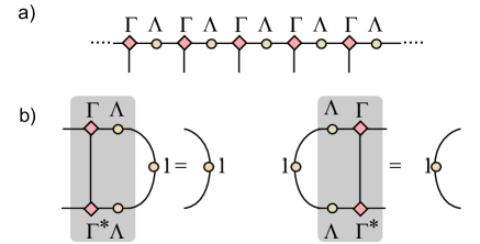
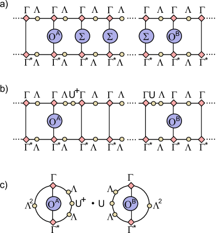
In this paper we follow Ref. Vidal, 2007 and use infinite matrix-product states (iMPS’s) for translationally invariant, infinite chains. In the iMPS representation, we write the matrices as a product of complex matrices and positive, real, diagonal matrices (see Fig. 1a for a diagrammatic representation). The matrices , can be chosen to be in a canonical form; that is, the transfer matrix
| (2) |
should have a right eigenvector with eigenvalue (∗ denotes complex conjugation). Similarly,
| (3) |
has a left eigenvector with (see Fig. 1b for a diagrammatic representation). In this case, the diagonal matrix contains the Schmidt values for a decomposition into two half infinite chains,
| (4) |
where and () are orthonormal basis vectors of the left and right partition, respectively. The states and can be obtained by multiplying together all the matrices to the left and right of the bond, e.g., if the broken bond is between sites and , the right Schmidt states are given by
| (5) |
Here, is the index of the row of the matrix; when the chain is infinitely long, the value of affects only an overall factor in the wavefunction. Reviews of MPS’s as well as the canonical form can be found in Refs. Perez-Garcia et al., 2007; Orús and Vidal, 2008; Vidal, 2007.
Furthermore, we must require that our state is not a cat state. The condition turns out to be that is the only eigenvector with eigenvalue .Pérez-García et al. (2008) The second largest (in terms of absolute value) eigenvalue determines the largest correlation length
| (6) |
II.2 Symmetry protected topological phases
If a state is invariant under an internal symmetry, which is represented in the spin basis as a unitary matrix , then the matrices must transform under in such a way that the product in Eq. (1) does not change (up to a phase). Thus the transformed matrices can be shown to satisfyPollmann et al. (2010); Pérez-García et al. (2008)
| (7) |
where is a unitary matrix which commutes with the matrices, and is a phase factor(see Fig. 2a for a diagrammatic representation). As the symmetry element is varied over the whole group, a set of phases and matrices and results. The phases form a 1D representation (i.e., a character) of the symmetry group. The matrices form a dimensional (projective) representation of the symmetry group. A projective representation is like an ordinary regular representation up to phase factors; i.e., if , then
| (8) |
The phases can be used to classify different topological phases.Pollmann et al. (2010); Schuch et al. (2011); Chen et al. (2011a) Consider for example a model which is invariant under a symmetry of rotations and . The phases for each spin rotation individually (e.g., ) can be removed by redefining the phase of the corresponding -matrix. However, the representations of and can also differ by a phase, which it turns out must be :
| (9) |
I.e., the matrices either commute or anti-commute. This resulting phase cannot be gauged away because the phases of and enter both sides of the equation in the same way. Thus we have two different classes of projective representations.
We can derive a similar relation to Eq. (7) for time reversal and inversion symmetry.Pollmann et al. (2010) For a time reversal transformation is replaced by (complex conjugate) on the left hand side. In the case of inversion symmetry is replaced by (transpose) on the left hand side of Eq. (7). In both cases we can distinguish the two different phases depending on whether and . Details on the classification of topological phases can be found in, e.g., Ref. Pollmann et al., 2010; Chen et al., 2011a, b; Schuch et al., 2011; Pollmann et al., 2012.
III Detecting symmetry protected topological phases in MPS representations
The definitions in the previous section tell us exactly what kind of topological phases exist in 1D and how to classify them. It does, however, not give us a direct method to detect and distinguish different phases. In Ref. Pollmann et al., 2010 it is pointed out that topologically non-trivial phases must have degeneracies in the entanglement spectrum. However, this does not distinguish among various non-trivial topological states (when there is more than 1). Furthermore, DMRG calculations sometimes produce states which have a degenerate entanglement spectrum for another reason (such as “cat states” for a phase with broken symmetry).
In this section we show to directly obtain the projective representations , given that the ground-state wave function is given in the form of an iMPS, i.e., we have access to the matrices. These matrices can be conveniently obtained using various numerical methods, e.g., the infinite time-evolving block decimation (iTEBD) method.Vidal (2007) The iTEBD method is a descendent of the density matrix renormalization group (DMRG) method.White (1992) Once the algorithm has converged to the ground state, the matrices are already in the desired canonical form.
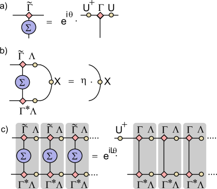
We will now explain how the -matrices may be obtained by diagonalizing transfer matrices.Pérez-García et al. (2008) First of all, we need to test if the iMPS is invariant under certain symmetry operations, i.e, we require that with being the transformed state. This implies that a “generalized” transfer matrix
| (10) |
must have a largest eigenvalue ,
| (11) |
see also the diagrammatic representation in Fig. 1b. Here is an internal symmetry operation and is equal to , or , depending on the symmetry of the system (the complex conjugate and transpose are required for time reversal and inversion, respectively). If , the overlap between the original and the transformed wave function decays exponentially with the length of the chain and is thus not invariant. Given that , the information about the symmetry protected topological phase of the system is encoded in the corresponding eigenvector . We will now see that is related to , specifically
| (12) |
(For DMRG calculations of , it is helpful to note that if the iMPS is not obtained in the canonical form, we need to multiply by the inverse of the eigenstate of the transfer matrix Eq.(2).)
This convenient expression for finding can be understood from the symmetry transformation of the Schmidt states defined in Eq. (5). Figure 1c shows the overlap of the Schmidt states with their transformed partners . The overlap corresponds to applying the generalized transfer matrix many times; hence only the dominant eigenvector remains in the thermodynamic limit. On the other hand, we can apply the transformation Eq. (7) to each transformed matrix and see that only the at the left end remains (Fig. 1d). Using the fact that the matrices , are chosen to be in the canonical form, we can read off that (where we normalize such that and ignore a constant phase factor which results from the right end). Thus the matrices can be obtained by finding the dominant eigenvector of the generalized transfer matrix, i.e., . Once we have obtained the of each symmetry operation, we can read off in which phase the state is. Furtermore, we can directly see the block structure of the matrices which is discussed in Ref. Pollmann et al., 2010.
III.1 Example: spin-1 chain
In this section we show for an example how we can use this approach to distinguish different symmetric phases. We consider the spin-1 model Hamiltonian
| (13) |
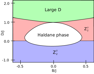
as a specific example in which symmetry protected topological phases occur. This model is invariant under translation, under spatial inversion as well as under a combined rotation around the -axis and complex conjugation []. The phase diagram has been studied in Ref. Gu and Wen, 2009 and is shown in Fig. 3. The point is the Heisenberg point, around which one finds the gapped Haldane phase. When increases, there is a transition into another phase which also does not break any symmetry. Even for , there is a transition between these two phases (with an intervening phase). At large , the phase is trivial and can be visualized by a state where all the sites are in the state, hence the phase containing the Heisenberg point seems to be a non-trivial topological phase. Furthermore, two antiferromagnetic phases and with spontaneous non-zero expectation values of and are present, respectively.
We now show how to use the method introduced in the previous section to distinguish different symmetry protected topological phases in the spin-1 model. In the presence of a symmetry (), we can use the symmetry operations and (or alternatively any other pair of orthogonal spin rotations) to calculate the matrices and as above. From them we can then define a quantity which distinguishes the different topological phases:
| (14) |
Here , are the largest eigenvalue of the generalized transfer matrix Eq. (2). Thus if the state is not symmetric and the two symmetric phases are distinguished by the properties of the matrices. If and commute () the system is in a trivial phase (i.e, same class as a site factorizable state) and if they anti commute (), the system is in a nontrivial phase (i.e., the Haldane phase). We proceed in a similar way for the other symmetries. In the presence of inversion symmetry (i.e., ), we define
| (15) |
For time reversal symmetry the matrices transformation as and the corresponding order parameter reads
| (16) |
These quantities behave similarly to , i.e., if the symmetry is broken and for the two symmetric phases.
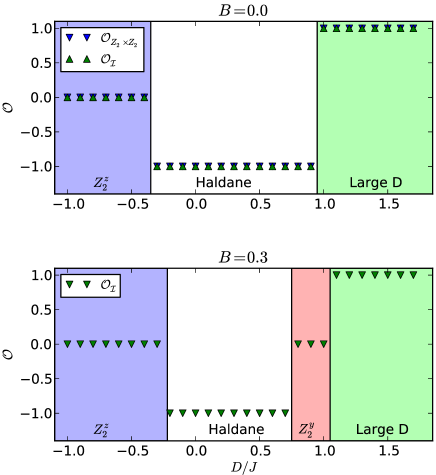
The procedure to calculate the quantities defined above is summarized by Eqs. (10), (11), (12) and the formulae Eqs. 14-(16) for the appropriate symmetry. We use the iTEBD methodVidal (2007) to obtain the ground state of Hamiltonian Eq. (13) in the desired canonical form. Then we construct the generalized transfer matrices Eq. (10) for the appropriate symmetry operations and find their largest eigenvalues with corresponding eigenvectors (Eq. (11)) using sparse matrix diagonalization (the iTEBD algorithms breaks the translational symmetry, yielding two matrices and thus we construct the transfer matrix using a two-site unit cell). From and we determine the quantities defined in Eqs. (14) and (15). Figure 4 shows the results which distinguish the phases clearly. Interestingly, the sharp distinctions between the phases can be achieved using MPS with rather small bond dimensions (we used MPS’s with up to only ).
IV Non-local order parameters from a wave function
In the previous section we showed how to detect different phases from an iMPS representation of the ground state. Now we derive expressions which can be evaluated when the wave function is given in another form, for example, using Monte Carlo or possibly experimentally (as proposed by Ref. Endres et al., 2011). The basic idea is to find some operators on the physical Hilbert space which give us some access to the -matrices which live in the “entanglement Hilbert space.”
IV.1 String order in the presence of internal symmetries
Perez-Garcia et al. Pérez-García et al. (2008) showed that the string order parameter, which was originally defined for symmetric spin chains den Nijs and Rommelse (1989) , can be generalized for systems with other symmetry groups. The generalized form for a state which is invariant under symmetry operations reads:
| (17) |
The non-vanishing of this expression for generic operators only means that the state is symmetric, but does not distinguish among topologically distinct states.
Nevertheless, we will now show that if the operators are chosen appropriately, this order parameter can distinguish some topological states. However, it is not a complete characteristization since we give an example below showing that it does not necessarily work in the presence of more complicated symmetries.
The most basic result about the string order correlator Eq. (17) is that a phase must be symmetric under for the string order to be non-zero. However, there is a second more refined condition for when the string order is nonzero, which can be used to distinguish between different symmetric phases. For example, the string order defined by vanishes in the large phase. Why does this occur even though the state is symmetric? The same string order is non-zero in the Haldane phase, hence it seems to be connected to the topological order of the phase, as we will show now.
Intuitively, the string order corresponds to calculating the overlap between the wave function with applied to consecutive sites and the wave function itself. Since is a symmetry of the wave function, it does not change anything in the bulk and the overlap should not vanish, generically speaking. A diagrammatic representation of the string order is shown in Fig. 5a. We represent the symmetry that is sandwiched in the middle using Eq. (7), i.e., . Ignoring the overall phase factor , we obtain the expression shown in Fig. 5b. If is large, the part in between the and is a product of orthogonal Schmidt states of the segment yielding a scalar product of delta functions on the left and on the right, yielding Fig. 5c. That is, the string order is equal to the product (where , or explicitly with the generalized transfer matrix as defined in Eq. (10), and where ). This expression is nonzero unless one of the two factors is equal to zero. Thus, the string order is generically non-zero in a symmetric phase.
Whether the factors vanish depends on the symmetry of the operators and can be seen as a selection rule for string order. Such selection rules exist only in the presence of additional symmetry. Thus, suppose that there are two symmetry operations and which commute but . We consider the string correlator , and focus on the left side of it. The operator can be chosen as having a particular quantum number under , i.e., . Then a short calculation shows that transforms in the same way under , . It follows that
| (18) | |||||
Thus we obtain a string order selection rule: the string order parameter vanishes if . Without the second symmetry , the string order would not vanish. Hence a nonzero string order in a state (though intuitively surprising) is actually not so unusual; it is the vanishing of a string order that is the signature of a topological phase. To summarize, the second criterion for the string order is that or else the string order vanishes.
The string order for the spin-1 Heisenberg chain can, for example, be derived simply in this way. Consider the Heisenberg chain with the symmetries and . Then the selection rule implies that the string order vanishes in the trivial phase if one of the operators , is odd under flips about the axis. The string order vanishes in the nontrivial phase if one of these operators is even (since is odd under flips about the -axis in this phase). Thus, vanishes in the nontrivial () phase and does not, while the situation is reversed in the trivial () phase. This is different than ordinary ordering transitions as, e.g., for the Ising model, where even operators have long-range correlations in both phases.
This approach may be used to give an order parameter that is sensitive to certain phase factors, those of the form for commuting symmetries. In order to determine systematically, find test operators with each possible transformation under , and then see which of these has a non-zero string correlation. In more detail, note first that where is the order of and where is some integer, and thus finding is equivalent to finding . We can then choose “test operators” that are powers of a single operator that transforms as . For calculate the string order with , translated to the left end of the segment, and , translated to the right end. The result will be nonzero only for one value of , namely .
In general, the possible phases of a system with a given symmetry group can be classified by finding all the consistent phase factors for a projective representation (see Eq. (8)). A phase can thus be identified by measuring the gauge-invariant combinations of these phase factors. The procedure just given works for phase factors that arise from a pair of symmetries that commute in the original symmetry group. However, for complicated groups, these might not be the only parameters that one needs. If and do not commute, e.g. (another symmetry), then there can be a phase in the projective representation, . This phase cannot be detected using the string-order selection rule, but it also does not matter since it is not gauge invariant: it can be absorbed into . To give an example of a gauge invariant phase that cannot be detected by a selection rule, we need to involve more symmetries. Suppose there is another pair of symmetries and with the same commutator, i.e., . Then in the projective representation, . Either or may be absorbed into , but not both. In fact, we can write:
| (19) |
Thus, is an example of a phase factor that is gauge invariant but cannot be detected by the string order just developed. (Appendix Acknowledgment fleshes out the details of this example.) This phase factor can be detected by the general approach we started with, of diagonalizing transfer matrices to find the ’s, and then just calculating the appropriate products of them.
At the end of the next section, we will describe another type of non-local order parameter that is sensitive to these more complicated local phase factors. Similar types of order parameters can also be used to identify phases protected by time reversal or inversion symmetry. In fact, these types of order parameter can detect any gauge-invariant phase-factor, so they give a complete way to determine what type of symmetry-protected topological order a system has.
IV.2 Non-local order parameters that measure the phase factors
Phases that are protected by inversion symmetry, time-reversal symmetry or more complicated internal symmetries (see example above) cannot be detected using the selection rules. However, there is another type of non-local order parameter (for example introduced by Ref. Cen, 2009 for inversion). The important thing about this parameter is not whether it vanishes, but what its complex phase is. The phase is simply equal to a gauge-invariant phase in the projective representations, such as the sign of .
Inversion symmetry.
In this case we can define an order parameter by simply reversing a part of the chain with an even length and then calculating the overlap:
| (20) |
where is the inversion on the segment from to . This expectation value can be evaluated using, e.g., Monte Carlo methods and it distinguishes the two possible symmetric phases by
| (21) |
where is a diagonal matrix which contains the Schmidt values (as defined in Sec. II). The sign of this quantity determines which of the two inversion-protected phases the chain is in. can be described by the following thought experiment: Form pairs of sites that are symmetric about the midpoint of the segment, and perform a measurement of the parity of the state of each pair. Then is . A non-zero value for means that there is a non-local correlation according to which the number of odd pairs is more likely to be either an even or odd number, even when the chain is very long. The effect is not so easy to see experimentally, since independent errors in measuring individual pairs will make even and odd numbers equally likely.
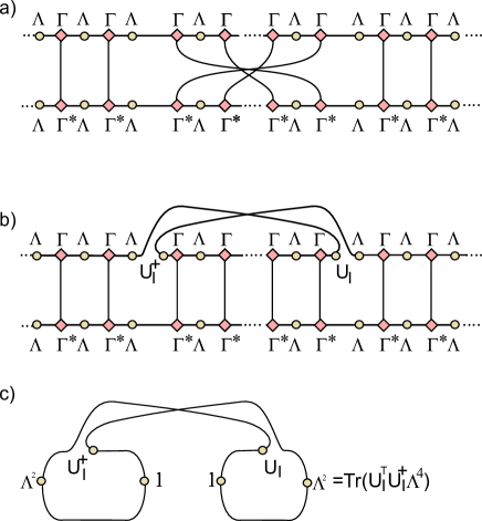
We now derive the string order formally using the iMPS representation together with the identities defined in Sec. II. The result of reversing a segment and taking the overlap, shown in Fig. 6a, is that the segments attaching the two chains to each other get twisted. These may be untwisted by reversing the orientation of the segment on the top level of the chain, at the expense of introducing a twist in it (see Fig. 6b); the explicit calculation uses the relationship , and so factors of appear in the diagram. Now, each of the ladders is a product of several copies of the transfer matrix , and so, if is large, it becomes a projection onto the largest eigenvector of , which is (see Eq. (2)), allowing the diagram to be simplified again (see Fig. 6c and Fig. 6d). Reading along the loop in this figure gives the value of the string order parameter:
| (22) |
Note that the line goes backwards through so it is transposed. Unlike the ordinary string order (which vanishes in one phase), it is the sign of this parameter that distinguishes among phases. (The factors of cancel.)
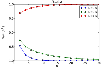
As a specific example, we calculated for the spin-1 Heisenberg chain (13) in the presence of a finite transverse field. In this case, the Haldane phase is stabilized by inversion symmetry. The results, which have been obtained using the iTEBD algorithm, are shown in Fig. 7. The order parameter shows a clear distinction between the two phases. As we approach the phase transition, the correlation length gets longer and we have to make the segment longer to see the convergence of to .

Time Reversal.
A more complicated expectation value can be used to distinguish between phases protected by time reversal symmetry. This order parameter is more subtle to devise because there is no way to apply time-reversal to just a portion of a system (as there is for inversion symmetry) since time-reversal is anti-unitary. For example, consider the state:
| (23) |
formed from two q-bits. One cannot apply time-reversal symmetry to just the first q-bit in a unique way, since the result of applying to just the first atom comes out differently for the two ways of grouping the factors. However, there is a way to express the overlap on the full chain without using antiunitary operators, and this is the starting point for a non-local order parameter. Consider for example a single spin with . Then
| (24) |
is not the ordinary expectation value of because both factors of have complex conjugates. To relate this to an expectation value, let us take two copies of the system and introduce the two states,
| (25) | |||||
| (26) |
so that . The phase of is not well-defined, since it depends on how one chooses the phase of so is a more useful quantity. This can be related to an experiment where one takes two unentangled copies of the system and measures their state in a basis including . The probability that the state is is then given by .
Now the generalization of to an entire chain is useful for testing whether time-reversal is broken spontaneously, but it does not help to distinguish between different phases. For that, an operator has to be applied over part of the chain in order to create “domain walls” which depend on . Therefore, we introduce an entangled state on just sites,
| (27) |
To define an order parameter that can distinguish different symmetric phases, we also have to introduce a swapping operator (defined similarly to Ref. Isakov et al., 2011). Let swap the parts of the chains between and . Then we find that
| (28) | |||||
with being the local dimension of the Hilbert space.The swapping operator is introduced because, without it, does not depend on the sign of (it is clearly positive). Multiplying by makes it possible to isolate the phase .
Figure 8 shows how to work out the order-parameter . The expectation value is evaluated in two parts: First, we calculate (Fig. 8a) and then (Fig. 8b). Since extends only over sites, these are partial inner products, giving a wave-function in which spins have been removed. The short sticks coming out of the other sites represent the sites that have not been contracted yet. Next, we transform Fig. 8a using Eq. (7) in the conjugate form and take the overlap between Figs. 8a and 8b, by contracting the short sticks with one another. There will be three “domain-wall” regions that we have to concentrate on (the bonds between ; and ); everything else can be simplified by replacing the ladders by projections onto the identity (in the same way as we have done several times before). The three “domain walls” can be replaced by the product of loops in Fig. 8c. Contracting these expressions gives , which is equal to Eq. (28). (If the swap had not been included, the domain wall on the right of the region contracted with would be proportional to . The swap reverses the orientation of one of the paths so that appears instead of , yielding the desired phase factor.) This string order is nonzero in both the time-reversal-protected phases, but when it is negative, the phase is non-trivial, just as for the inversion-symmetry.
Combinations of Multiple Local Symmetries
A similar type of string order expectation value can also be used to identify more tricky phase factors, like in Eq. (19). This type of string order was introduced by Ref. Haegeman et al., 2012. To be general, note that there is a gauge invariant phase any time there is a sequence of symmetries which can be multiplied together to give the identity in more than one way, (where the indices are a permutation of ). When these symmetries are replaced by the ’s, a phase factor appears, , and the phase factor is gauge invariant. For example, in Eq. (19), the symmetries can be multiplied together in the order which gives the identity by assumption or each symmetry can be grouped with its inverse, which also cancels to . We will now see that such phase factors can be identified by taking multiple chains and applying symmetries and permutations to them. The point we would most like to make about this order parameter is that it succeeds at identifying phase factors that the string order selection rule fails to detect. In fact, it gives a complete way to distinguish between topological states, because Schur showed that every gauge-invariant phase factor in a projective representation has this form, see Appendix B.
The string order is illustrated in Fig. 9 for .
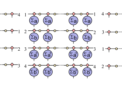
Take identical copies of the given state, and place them side-by-side. Take three successive long segments , and . Now apply the symmetries to the middle segment and different permutations to the two ends (similar to the swap operator used in the case of time reversal symmetry). This causes the matrices at each of the ends of to get multiplied together in two orders which allows one to detect the phase factor. Fig. 9 illustrates the order parameter for the simplest case of (where and commute). The order parameter and its value is
| (29) | |||||
Here consists of permuting the left segments of the chains according to the permutation (written as a cycle), means to apply the symmetry to the middle segment of the chain, and indicates permuting the right segments. The wave function is simple a product of replicas of the ground state. To identify the phase factor in Eq. (19), take chains, and apply the symmetries to the legs of the ladder in the middle segment. Then apply the permutations on the left segment and on the right one, in order to get the ’s to cancel with their inverses on the right and to obtain on the left, which is the phase we want to find. (We could also apply a bunch of two cycles on the right end to get the same phase factor but multiplied by a different combination of Renyi entropies.)
This type of nonlocal order parameter distinguishes between all phases with a local symmetry group. Time reversal and inversion symmetry phase factors can be determined as in the previous section. By combining all these ideas together, it should also be possible to measure phase factors that arise from combining spatio-temporal symmetries with local symmetries. (We have not yet worked out order parameters for groups that contain either inversion or time-reversal symmetry together with local symmetries, but it seems likely to be possible.)
V Conclusions
A topological phase is a phase of matter which cannot be characterized by a local order parameter. Gapped phases in 1D systems can be completely characterized using tools related to projective representations of the symmetry groups. If the ground state is given in the form of a matrix-product state representation, the different topological phases can be directly detected by diagonalizing a generalized transfer matrix (obtained from an overlap with the transformed matrix-product state). Based on this fact, we also introduced non-local order parameters which can be simply calculated using alternative representations. Such an order parameter could be determined for a wave function using Monte Carlo simulations or possibly experimentally. The ordinary string order for the Haldane phase can be explained using a selection rule that changes at the critical point: there are two types of string orders (depending on the operators at the ends of the string), one which vanishes in the trivial phase, and one which vanishes in the non-trivial one. This order parameter can be generalized to many cases, but not to all groups. An alternative order parameter that directly measures the “projective phases” is required to distinguish among phases in general. Such an order parameter work for all cases, including time reversal, inversion symmetry, and complicated local symmetry groups. Intriguingly, this parameter involves measuring expectation values of string operators on multiple copies of the system, even though these copies are uncorrelated.
Acknowledgment
We thank Erez Berg and Masaki Oshikawa for useful discussions and the collaboration on a related project. A.M.T. acknowledges the hospitality of the guest program of MPI-PKS Dresden.
Appendix A Example of a Phase that cannot be detected by String Order Selection Rules
Let us assume that a state is invariant under a symmetry group which fulfills the group algebra . (We simplify the expressions by writing instead of .) Then is gauge-invariant and does not look easy to detect by using the selection rule for string order from Sec. IV.1. But this is not completely obvious. In fact, if and both commute with both and , then we can rearrange into . Thus and commute, allowing us to define a phase (in general, we define for commuting symmetries as the phase of ). The phase can be expressed in terms of it. In fact, rearranging the expression for and remembering to keep track of the phases that might arise from exchanging e.g. and (on account of the topological order), we find that , so reduces to simpler phase-factors which can all be determined by using the string order selection rule.
More pairs of symmetries must be non-commuting to ensure that there is no way to simplify . We will introduce the following group algebra, with and relabeled and ,
| (30) |
Besides the original symmetries we have introduced additional symmetries as the commutators of some of them. Aside from these conditions, we assume that all the generators square to one. This group has elements. The algebraic relations defining it are complicated generalizations of the quaternion group; for example, the first equation corresponds to the commutator of and being , which commutes with everything and squares to like does.
Example of “undetectable” projective phase factors for this group: We can write the elements in the group as products of and . The numbers of factors are each the same modulo two no matter how we rearrange the factors. So define and to be the number of ’s and ’s appearing modulo 2. Assume the following projective phase factors:
| (31) |
(To create an example of an undetectable phase factor, we want a minus sign to appear in the first of Eqs. (30) on replacing the symmetries by their matrices, and we want this to be the only phase factor that appears. These conditions lead to Eq. (31).) It is easy to check that this definition is consistent, i.e., that The calculation starts from the linearity of and , e.g. .
Now let us show first that this is a non-trivial phase (by showing that there is a non-trivial phase factor defined using four symmetries) and second that this phase cannot be detected using a string order selection rule, because all the commuting pairs of elements and also commute in the projective representation. Hence this is a nontrivial phase without any signature in the ordinary string order.
The phase is non-trivial as while . Hence the gauge-invariant phase factor from these four symmetries is .
However, all two-symmetry phase factors are trivial. To show this, we have to enumerate (at least partly) all the pairs of symmetries that commute, and then check that the ’s for them also commute. Write and where the ’s are each or and the ’s are products of some combination of , and (i.e., elements of the center of the group). Since the commutators of any two of are in the center, the commutator of and can be calculated by evaluating the commutators of their factors one pair at a time:
| (32) |
We want and to commute, so the exponents of ,, must be zero modulo 2. We will then want to calculate . which according to Eq. (31) is .
In order for and to commute, the exponents of the ’s must vanish:
| (33) |
Consider all four possible combinations of values for and . First, if , then and commute because . Second, if and , then we must have by Eq. (33). This implies that or . But this commutes with only in the former case (since has a factor of in it and this does not commute with ), while there is a non-trivial phase factor only in the latter case. The remaining two cases are similar.
Appendix B Schur’s Theorem on Projective Representations
Schur classified the types of projective representations (which are also known as the “Schur Multiplier”); the resultKarpilovsky (1987) shows that all one-dimensional phases, at least with local symmetry groups, can be recognized using the order parameter of Sec. IV.2. The gauge-invariant phase-factors we have found involve products such as where ,,, are generators of the group. This phase factor can be defined by listing the sequence of group elements that have to be multiplied together: , without actually multiplying them. It is convenient to regard such sequences as forming a group (a “free group”): to multiply two sequences, juxtapose them and cancel elements with their inverses when they meet each other. This structure is useful because it makes it possible to break phase factors down to simpler ones (for example, repeating the string just given twice does not give a new phase factor, just the square of the original one).
The sequences that give a gauge-invariant phase factor form a group, which Schur’s theorem describes. In general, let the symmetry group be and let be a set of symmetries that generate it; call the set of sequences of these generators the free group . Let be the group generated by commutators of two elements of . (Similarly, one can define the commutator of any two subgroups ). Consider also the set of sequences whose product is equal to the identity. A sequence that lies in both these subgroups determines a gauge-invariant phase factor; that is, there is a function defined on . Because is an element of , it gives a phase when the corresponding ’s are multiplied together, and these phases are invariant because elements of are products of commutators, that is, they have the form where the ’s and ’s are various elements of . The theorem of Schur states that all gauge-invariant phase factors are contained in this function. In addition, the theorem finds all the conditions that have to be satisfied by these phases (such as when one of the phases has to be ); the general rule is that when .
Hence, the classes of projective representations of a group are in one-to-one correspondence with characters on the group . When is finite, this is a finite group, too.
For example, consider . Let and be the two generators. Then is an element of because and commute as elements of the group . It is also an element of , so it defines a phase factor . Now the second part of the theorem implies that this phase factor is equal to . To see this, we will show that , which implies . That is implied by the following relationship (where the commas represent multiplication in the free group): . This is in because and are both in .
References
- Landau (1937) L. D. Landau, Phys. Z. Sowjetunion 11, 26 (1937).
- Wen (1989) X.-G. Wen, Phys. Rev. B 40, 7387 (1989).
- Haldane (1983a) F. D. M. Haldane, Phys. Lett. 93A, 464 (1983a).
- Haldane (1983b) F. D. M. Haldane, Phys. Rev. Lett. 50, 1153 (1983b).
- Affleck et al. (1987) I. Affleck, T. Kennedy, E. H. Lieb, and H. Tasaki, Phys. Rev. Lett. 59, 799 (1987).
- Affleck et al. (1988) I. Affleck, T. Kennedy, E. H. Lieb, and H. Tasaki, Commun. Math. Phys. 115, 477 (1988).
- den Nijs and Rommelse (1989) M. den Nijs and K. Rommelse, Phys. Rev. B 40, 4709 (1989).
- Pollmann et al. (2010) F. Pollmann, A. M. Turner, E. Berg, and M. Oshikawa, Phys. Rev. B 81, 064439 (2010).
- Turner et al. (2010) A. M. Turner, F. Pollmann, and E. Berg, arXiv:1008.4346 (2010).
- Chen et al. (2011a) X. Chen, Z. Gu, and X. Wen, Physical Review B 83, 035107 (2011a).
- Chen et al. (2011b) X. Chen, Z. Gu, and X. Wen, arXiv:1103.3323 (2011b).
- Schuch et al. (2011) N. Schuch, D. Pérez-García, D.ia, and I. Cirac, Phys. Rev. B 84, 165139 (2011).
- Pérez-García et al. (2008) D. Pérez-García, M. Wolf, M. Sanz, F. Verstraete, and J. Cirac, Phys. Rev. Lett. 100, 167202 (2008).
- Haegeman et al. (2012) J. Haegeman, D. Perez-Garcia, I. Cirac, and N. Schuch, ArXiv e-prints (2012), eprint 1201.4174.
- Endres et al. (2011) M. Endres, M. Cheneau, T. Fukuhara, C. Weitenberg, P. Schauß, C. Gross, L. Mazza, M. C. Bañuls, L. Pollet, I. Bloch, et al., Science 334, 200 (2011),
- Cen (2009) L.-X. Cen, Phys. Rev. B 80, 132405 (2009).
- Fannes et al. (1992) M. Fannes, B. Nachtergaele, and R. W. Werner, Commun. Math. Phys. 144, 443 (1992).
- Vidal (2007) G. Vidal, Phys. Rev. Lett. 98, 070201 (2007).
- Hastings (2007) M. B. Hastings, J. Stat. Mech. 2007, P08024 (2007).
- Gottesman and Hastings (2009) D. Gottesman and M. B. Hastings, arXiv:0901.1108 (2009).
- Schuch et al. (2008) N. Schuch, M. M. Wolf, F. Verstraete, and J. I. Cirac, Phys. Rev. Lett. 100, 030504 (2008).
- Perez-Garcia et al. (2007) D. Perez-Garcia, F. Verstraete, M. Wolf, and J. Cirac, Quantum Inf. Comput. 7, 401 (2007).
- Orús and Vidal (2008) R. Orús and G. Vidal, Phys. Rev. B 78, 155117 (2008).
- Pollmann et al. (2012) F. Pollmann, E. Berg, A. M. Turner, and M. Oshikawa, Phys. Rev. B 85, 075125 (2012).
- White (1992) S. R. White, Phys. Rev. Lett. 69, 2863 (1992).
- Gu and Wen (2009) Z.-C. Gu and X.-G. Wen, Phys. Rev. B 80, 155131 (2009).
- Isakov et al. (2011) S. V. Isakov, M. B. Hastings, and R. G. Melko, Nature Physics 7 (2011).
- Karpilovsky (1987) G. Karpilovsky, The Schur multiplier, LMS monographs (Clarendon Press, 1987), ISBN 9780198535546,