Sensing and Multiscale Structure

Abstract

We introduce a method of estimating parameters associated with a fractal random scattering medium, which utilizes the multiscale properties of the scattered field. The example of ray-density fluctuations beyond a phase screen with fractal slope is considered. An exact solution to the forward problem, in the case of the Brownian fractal, leads to an expression for the volatility of the slope. This expression is invariant under a change of probability measure, a fact which gives rise to the corresponding result for a (stationary) Ornstein-Uhlenbeck slope. We demonstrate that our analytical results are consistent with numerical simulations. Finally, an application to the determination of sea ice thickness via sonar is discussed.

1 Introduction

When a wave is scattered by a random medium the scattered radiation can be described by a random field. We consider the problem of estimating parameters related to the characteristics of the scattering medium. The numerous applications of such problems, for example, in the areas of industry, geophysics and medicine are well known, and are of considerable practical importance [1].

One possible approach is the following: First, derive an expression for the “random scattered field”, or some observable properties thereof. Then, compare these theoretical quantities with the corresponding sample quantities derived from experiment. A popular version of this strategy is the “method of moments” which uses the mean, variance, correlation function etc. A refinement of this, also along Bayesian lines, is the method of maximum likelihood, which can provide optimal estimates of the parameters in question [2]. However, this technique is not usually available in scattering problems. Elementary considerations soon lead to the conclusion that scattered fields (arising from, for example, a homogeneous random scattering medium) are rarely endowed with convenient properties. For instance, in the example of surface scattering the Markov property will not hold in general, since the scatter could be a function of the whole of the scattering surface.

If the scattered field has fractal properties, there is another possibility for estimating parameters, unrelated to Bayes theorem. Information can be derived from fluctuations in the field at all scales. The principle can be understood by relation to the “well known fact” that the volatility of an Ito diffusion can be recovered with probability one, given a sample path over any non-zero interval, see e.g. [3]. It is common for naturally occurring structures to possess multiscale character suitable to be modeled as a fractal. Moreover, it seems reasonable to suppose that such structures might confer multiscale properties to the scattered field. Parameter estimation based around this idea is potentially very efficient, since it does not require the availability of data over many correlation lengths. This approach to sensing (inverse scattering) is apparently new, and is illustrated here through the example of ray-density fluctuations beyond a subfractal phase-changing screen (SPS). The concept of rays is of great utility in the theory of scattering, most famously in the shortwave limit [4], but also more generally [5]. The ray-density, denoted by $R$, describes intensity fluctuations induced by a SPS in an incoherent configuration (no interference). $R$ also features in expressions for the moments of the scattered intensity in a coherent configuration [6]. We consider scatter from a one-dimensional SPS in an incoherent configuration, which provides the simplest example of the proposed technique.

2 The phase screen model

When a plane of parallel rays passes through a non-flat refracting layer, differences in the refractive index of the layer cause the rays to scatter. The situation may be described by specifying the slope (gradient) of a surface of constant phase in terms of a one-dimensional stochastic process $(Y_{t})_{t\in\mathbb{R}}$. If $Y$ is fractal, then we have a “subfractal phase-changing screen” [6]. This model also describes surface scattering, when the source and point of observation are coincident, and shadowing and multiple scattering are neglected, see Fig. 1. These surfaces can be thought of as possessing a faceted structure, and have been used to model, among other things, scattering of radio waves in the ionosphere [7], and the effect of internal waves on acoustic propagation in the ocean [8].

\psfrag{A}[c]{{\small$a$}}\psfrag{B}[c]{{\small$\sigma$}}\includegraphics[width=433.62pt]{fig1.eps}

Figure 1: Rays scattered from a faceted random surface, or through a subfractal phase-changing screen.

The ray-density can be approximated at $a\in A_{n}:=[a_{n},a_{n+1})$ where $a_{n}=n\Delta a$, a unit distance from the layer by $\{\mathbf{R}_{n}^{Y}(\Delta t,\Delta a);n\in\mathbb{Z}\}$ defined as

$$\mathbf{R}_{n}^{Y}(\Delta t,\Delta a):=\frac{1}{\Delta a}\sum_{k=-\infty}^{\infty}\mathbf{1}_{\{t_{k}-{Y}_{t_{k}}\in A_{n}\}}\Delta t$$ (1)

where $t_{k}=k\Delta t$ and $\Delta a\gg\Delta t$. The ray-density $(R_{a}^{Y})_{a\in\mathbb{R}}$ is defined as the limit (when it exists)

$$R_{a}^{Y}:=\lim_{\Delta a\rightarrow 0}\lim_{\Delta t\rightarrow 0}\mathbf{R}_{n}^{Y}(\Delta t,\Delta a)=:\int_{\mathbb{R}}\mathrm{d}t\,\delta(Y_{t}-t+a)$$ (2)

where $a\in A_{n}$. Assume that $Y$ is an Ito diffusion described by the stochastic differential equation $\mathrm{d}Y_{t}=-\theta Y_{t}\mathrm{d}t+\sigma\mathrm{d}B_{t}$, where $(B_{t})_{t\in\mathbb{R}}$ is a Brownian motion, and $\theta\in[0,\infty)$ and $\sigma>0$ are parameters known as the damping and volatility respectively. Norris [9] found an exact solution to the forward problem when $\theta=0$, obtaining $R^{Y}$ when $Y_{t}=\sigma B_{t}$. This is referred to as the case of “Brownian slope”.

3 Brownian slope

The result from [9], that $R^{Y}$ is an Ito diffusion when $Y_{t}=\sigma B_{t}$ is stated briefly below:

The quantity

$$L_{t}^{x}:=\int_{0}^{t}\mathrm{d}s\,\delta(X_{s}-x)$$ (3)

known as the occupation density or local time, measures infinitesimally the “time spent at $x$ by $X$ before $t$”. Set $X_{t}=\sigma B_{t}-t$, where $(B_{t})_{t\geq 0}$ is a Brownian motion, started at zero. Also, let $T$ denote the first time that $X$ hits level $K<0$. It follows from the Ray-Knight theorem on Brownian local time, that the process $(L_{T}^{x})_{x\geq K}$ has generator

$$\mathscr{L}=\frac{2}{\sigma^{2}}\left[l\left(\frac{\mathrm{d}}{\mathrm{d}l}\right)^{2}+(\mathbf{1}_{\{x\leq 0\}}-l)\frac{\mathrm{d}}{\mathrm{d}l}\right].$$ (4)

Since $X_{t}\rightarrow-\infty$ as $t\rightarrow\infty$, $(X_{t})_{t\geq 0}$ has a final local time $F_{x}:=\lim_{t\rightarrow\infty}L_{t}^{x}<\infty$. Taking $K\rightarrow-\infty$, $(F_{x})_{x\in\mathbb{R}}$ is a diffusion, and $R_{a}^{\sigma B}=\lim_{b\rightarrow\infty}F_{-a-b}$ is a diffusion on $a\in\mathbb{R}$, with generator

$$\mathscr{L}=\frac{2}{\sigma^{2}}\left[r\left(\frac{\mathrm{d}}{\mathrm{d}r}\right)^{2}+(1-r)\frac{\mathrm{d}}{\mathrm{d}r}\right].$$ (5)

Now consider the problem of finding $\sigma$. Calling our probability measure $\mathbb{P}$, it follows immediately from (4) that $L_{T}$ satisfies

$$\sigma^{2}=4\int_{J}^{I}\mathrm{d}x\,L_{T}^{x}/\langle L\rangle_{J,I}\quad\mathbb{P}\mbox{-a.s.}$$ (6)

where $I>J>K$, and $\langle L\rangle_{J,I}$ denotes the quadratic variation of $L_{T}$ on $[J,I]$. Also, by sending $K\rightarrow-\infty$ in (6), or from (5), $R^{\sigma B}$ satisfies

$$\sigma^{2}=4\int_{I}^{J}\mathrm{d}a\,R_{a}/\langle R\rangle_{I,J}\quad\mathbb{P}\mbox{-a.s.}$$ (7)

for $I<J$. At first glance, the expression (7) might appear to be the end of the matter, but there is an important sense in which it is unphysical. A density is of course an idealization. In practice, one seeks an approximation by measuring the energy flux over some finite area. For a general density $(Z_{x})_{x\in\mathbb{R}}$ define the “discrete local average” $(\bar{Z}_{n})_{n\in\mathbb{Z}}$ by

$$\bar{Z}_{n}:=\frac{1}{\Delta a}\int_{A_{n}}\mathrm{d}x\,Z_{x}$$ (8)

where $\Delta a>0$ is the width over which the average is taken. The quantity $\bar{Z}$ is observable, and we assume that measurements of $\bar{Z}$ are available. Consider the case $Z=B$, a Brownian motion. One quickly finds that

$$\mathbb{E}[(\bar{B}_{n+1}-\bar{B}_{n})^{2}]=2\Delta a/3.$$ (9)

Define a partition of $[I,J]$ as $\{a_{n};n=n_{0},...,\tiny{N}\}$, and the quadratic variation of $\bar{Z}$ as

$$\langle\bar{Z}\rangle_{I,J}:=\lim_{\Delta a\rightarrow 0}Q_{I,J}(\bar{Z})$$ (10)

where

$$Q_{I,J}(\bar{Z}):=\sum_{n=n_{0}}^{N-1}(\bar{Z}_{n+1}-\bar{Z}_{n})^{2}.$$ (11)

It follows from (9) that $\langle\bar{B}\rangle_{I,J}\neq\langle B\rangle_{I,J}$. If $\langle\bar{B}\rangle_{I,J}$ is deterministic (9) implies that $\langle\bar{B}\rangle_{I,J}=2(J-I)/3$ $\mathbb{P}$-a.s.. This follows from the second moment method if

$$\lim_{\Delta a\rightarrow 0}\mathbb{E}[Q_{I,J}^{2}(\bar{B})]$$ (12)

$$= \lim_{\Delta a\rightarrow 0}\mathbb{E}[Q_{I,J}(\bar{B})]^{2}=4(J-I)^{2}/9.$$ (13)

The expectation in (12) is not as easy to evaluate as in the Brownian case (without the local average), since the increments $\bar{B}_{n+1}-\bar{B}_{n}$ are not independent. However, the (quadruple) integrals that result from multiplying out the squared sum are trivial to compute using the correlation function $\mathbb{E}[B_{s}B_{t}B_{u}B_{v}]=s(2t+u)$ where $0\leq s\leq t\leq u\leq v$. For example, for $n_{0}=0$, $N=1$ we have

$$\mathbb{E}[Q^{2}(\bar{B})]=\mathbb{E}\left[(\bar{B}_{1}-\bar{B}_{0})^{4}\right]$$

$$= \mathbb{E}\left[\bar{B}_{0}^{4}-2\bar{B}_{0}^{3}\bar{B}_{1}+6\bar{B}_{0}^{2}\bar{B}_{1}^{2}-2\bar{B}_{0}\bar{B}_{1}^{3}+\bar{B}_{1}^{4}\right].$$ (14)

Each of the terms in (14) can be evaluated by exchanging the order of the expectation and the integral, and time ordering. For example, the first term:

$$\mathbb{E}\left[\bar{B}_{0}^{4}\right]= \frac{4!}{(\Delta a)^{4}}\int_{0}^{\Delta a}\mathrm{d}v\int_{0}^{v}\mathrm{d}u\int_{0}^{u}\mathrm{d}t\int_{0}^{t}\mathrm{d}s\,\mathbb{E}[B_{s}B_{t}B_{u}B_{v}]$$

$$= (\Delta a)^{2}/3.$$ (15)

For larger values of $N$ one can use a computer to sum the terms and verify that $\mathbb{E}[Q_{I,J}^{2}(\bar{B})]$ does indeed appear to tend to the required limit (13). Taking this as an assumption, and applying the same reasoning to the process defined by (5), it follows from (7), in the limit $\Delta a\rightarrow 0$, that $\bar{R}^{\sigma B}$ satisfies

$$\sigma^{2}=\frac{8}{3}\int_{I}^{J}\mathrm{d}a\,\bar{R}_{a}/\langle\bar{R}\rangle_{I,J}\quad\mathbb{P}\mbox{-a.s.}$$ (16)

where $\bar{R}_{a}^{Y}:=\lim_{\Delta a\rightarrow 0}\bar{R}_{n}^{Y}=R_{a}^{Y}$ for $a\in A_{n}$. Hence (16) solves the inverse problem for the Brownian slope. Noting that $\bar{R}_{n}^{Y}=\lim_{\Delta t\rightarrow 0}\mathbf{R}_{n}^{Y}(\Delta t,\Delta a)$, $\bar{R}$ can be simulated using (1). Fig. 2 shows values of $\sigma$ computed using (16).

\psfrag{A}[c]{{\small$a$}}\psfrag{B}[c]{{\small$\sigma$}}\includegraphics[width=433.62pt]{fig2.eps}

Figure 2: Three values of $\sigma$ computed from (16) using (1) for Brownian slope. Note that the rate of convergence is only limited by the finiteness of $\Delta t$ and $\Delta a$. The Brownian motion is simulated exactly with $\Delta a=2\times 10^{-4}$ and $\Delta t=10^{-8}$.

The Brownian slope model is somewhat unsatisfactory since Brownian motion is non-stationary and $\lim_{t\rightarrow\infty}|B_{t}|=\infty$. Of greater verisimilitude is the model resulting when $\theta>0$, then $Y$ is a stationary Ornstein-Uhlenbeck (OU) process, a Gaussian Markov process with exponential autocorrelation function. This is referred to as the case of “OU slope” and is considered next.

4 OU slope

Define a probability measure $\mathbb{Q}$ such that $\mathrm{d}\mathbb{Q}:=M_{T}\mathrm{d}\mathbb{P}$. If $(M_{t})_{0\leq t\leq T}$ is a martingale then $\mathbb{P}$ and $\mathbb{Q}$ are equivalent which means that any event that has probability one w.r.t. $\mathbb{P}$ must also have probability one w.r.t. $\mathbb{Q}$. Let $(B_{t})_{t\geq 0}$ be a $\mathbb{P}$-Brownian motion, started at zero. Then $(M_{t})_{0\leq t\leq T}$ where

$$M_{t}=$$ (17)

$$\mathrm{exp}\left(-\theta\int_{0}^{t}\mathbf{1}_{\{s\leq-K\}}B_{s}\mathrm{d}B_{s}-\frac{\theta^{2}}{2}\int_{0}^{t}\mathrm{d}s\,\mathbf{1}_{\{s\leq-K\}}B_{s}^{2}\right)$$

is a martingale, which can be verified, for example, with the help of Example 3, p.233, [10]. Now, for the process $(X_{t})_{0\leq t\leq T}$ defined as above, it follows from the Girsanov theorem (see for example [3]) that

$$\mathrm{d}X_{t}=-\mathbf{1}_{\{t\leq-K\}}\theta(X_{t}+t)\mathrm{d}t-\mathrm{d}t+\sigma\mathrm{d}W_{t}\quad\mbox{w.r.t.}\,\,\mathbb{Q}$$ (18)

where $(W_{t})_{0\leq t\leq T}$ is a $\mathbb{Q}$-Brownian motion. The process $(U_{t})_{0\leq t\leq-K\wedge T}$ where $U_{t}:=X_{t}+t$ is a $\large\mathbb{Q}$-OU process, such that $\mathrm{d}U_{t}=-\theta U_{t}\mathrm{d}t+\sigma\mathrm{d}W_{t}$ w.r.t. $\mathbb{Q}$. By the equivalence of $\mathbb{P}$ and $\mathbb{Q}$, (6) implies that

$$\sigma^{2}=4\int_{J}^{I}\mathrm{d}x\,L_{T}^{x}/\langle L\rangle_{J,I}\quad\mathbb{Q}\mbox{-a.s.}$$ (19)

where $I>J>K$. Note that $L_{T}$ is not Markov under $\mathbb{Q}$. The remaining steps are understood to be w.r.t. $\mathbb{Q}$. Taking $K\rightarrow-\infty$, $(X_{t})_{t\geq 0}$ has a final local time $F_{x}<\infty$. Then, $R_{a}^{U}=\lim_{b\rightarrow\infty}F_{-a-b}$ where $(U_{t})_{t\in\mathbb{R}}$ is a stationary OU process described by $\mathrm{d}U_{t}=-\theta U_{t}\mathrm{d}t+\sigma\mathrm{d}W_{t}$, and $(W_{t})_{t\in\mathbb{R}}$ is a Brownian motion. It now follows from (19), in this limit, that $R^{U}$ satisfies

$$\sigma^{2}=4\int_{I}^{J}\mathrm{d}a\,R_{a}/\langle R\rangle_{I,J}\quad\mathbb{Q}\mbox{-a.s.}$$ (20)

for $I<J$. Then, noting that the change-of-measure argument goes through as above, and assuming (13), $\bar{R}^{U}$ satisfies

$$\sigma^{2}=\frac{8}{3}\int_{I}^{J}\mathrm{d}a\,\bar{R}_{a}/\langle\bar{R}\rangle_{I,J}\quad\mathbb{Q}\mbox{-a.s.}$$ (21)

where $\bar{R}_{a}$ is defined as in (16). Hence $\sigma$ can be obtained given the ray-density on any non-zero interval in the case of OU slope, see Fig. 3. We emphasize that the expression is valid for arbitrary $\theta\in[0,\infty)$.

\psfrag{A}[c]{{\small$a$}}\psfrag{B}[c]{{\small$\sigma$}}\includegraphics[width=433.62pt]{fig3.eps}

Figure 3: Three values of $\sigma$ computed from (21) using (1) for OU slope. As in the Brownian case, the rate of convergence is only limited by the finiteness of $\Delta t$ and $\Delta a$. The OU process is simulated exactly with $\Delta a=2\times 10^{-4}$ and $\Delta t=10^{-8}$.

With regard to $\theta$, consider the moments of $\bar{R}^{U}$. It is not hard to see that the moments of $\bar{R}^{U}$ are equal to the moments of $R^{U}$ in the limit $\Delta a\rightarrow 0$. Therefore, for ease of calculation, the moments of $R^{U}$ are considered, and the superscript is dropped to aid clarity. One quickly finds that $\mathbb{E}[R]=1$. For the second moment, define the process $\{R_{a}(t_{0});a\in\mathbb{R}\}$ as

$$R_{a}(t_{0}):=\int_{t_{0}}^{\infty}\mathrm{d}t\,\delta(U_{t}-t+a).$$ (22)

where $U$ is an OU process with transition density

$$\rho(U_{t}=y|U_{s}=x)=$$ (23)

$$\frac{\sqrt{\theta}}{[\pi\sigma^{2}(1-e^{-2\theta|t-s|})]^{1/2}}\mathrm{exp}\left[-\frac{\theta(y-xe^{-\theta|t-s|})^{2}}{\sigma^{2}(1-e^{-2\theta|t-s|})}\right]$$

see for example [11]. For $X_{t}:=U_{t}-t$, it follows that

$$\mathbb{E}[R_{a}^{2}(t_{0})|\{X_{t_{0}}=x_{0}\}]$$ (24)

$$= 2\int_{-a}^{\infty}\mathrm{d}q\,\rho(U_{q+a}=q+t_{0}|U_{0}=u_{0})\mathbb{E}[R_{q}(t_{0})|\{X_{t_{0}}=q\}].$$

The unconditional second moment can be found by taking $t_{0}\rightarrow-\infty$, or, equivalently, by fixing $t_{0}=0$ and sending $a\rightarrow\infty$:

$$\mathbb{E}[R^{2}]=\lim_{a\rightarrow\infty}\mathbb{E}[R_{a}^{2}(0)|\{X_{0}=q\}]$$

$$= 2\int_{\mathbb{R}}\mathrm{d}q\,\rho(U=q)\mathbb{E}[R_{q}(0)|\{X_{0}=q\}]$$ (25)

where $\rho(U=q)$ is the point-density of the long-term limit of $U$. This calculation is similar to the Kac moment formula [11]. In general (25) must be evaluated numerically. An approximate analytical result is available when the correlation length of $U$ is small compared to the height of the point of observation above the surface, that is $1/\theta\ll 1$. Assume for simplicity that $\sigma^{2}\sim 1$, then

$$\lim_{\Delta a\rightarrow 0}\mathbb{E}[\bar{R}^{2}]=\mathbb{E}[R^{2}]\simeq 1+\frac{1.1}{\sqrt{\theta\sigma^{2}}}$$ (26)

holds to a close approximation for $\theta\gtrsim 10^{2}$, see Fig. 4. Finally, (26) combined with (21) provides a way to estimate of $\theta$ given $\sigma$.

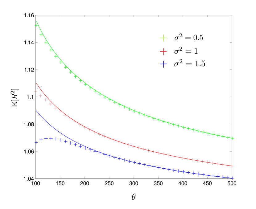
Figure 4: (color online) An approximate expression for the second moment. Solid lines are (26). The ‘$+$’ denote exact values from numerical integration of (25).

5 Application to sensing of sea ice thickness and discussion

An example of an application is the following: The first convincing evidence for the thinning of the Arctic sea ice was collected using submarine mounted sonar [12]. Sonar methods continue to this day to provide the most reliable source of information on sea ice thickness on large scales [13]. The thickness of the ice can be inferred from the range of the mean surface of the underside. This surface is known to possess fractal properties, and to have an approximately exponential correlation function [14]. The statistics of the ice surface are important parameters for determining the relation between the range and the time elapsed before the earliest return [15]. Typically, returns from various reflecting points are resolvable in time. It follows that the individual intensities can be added, the sum being proportional to the ray-density, assuming the geometrical optics approximation. Taking the OU process as a one-dimensional model of the slope of the surface, estimates of $\{\sigma,\theta\}$ can be obtained given $\bar{R}^{U}$ as outlined above.

To summarize, the example provided exploits fluctuations in the ray-density, which is proportional to the intensity in incoherent configurations. The potential scope of the method is clearly far wider than the example given. As already mentioned, the ray-density features in expressions for the moments of the intensity in coherent configurations, in the short wavelength limit. Furthermore, it is $R$ which appears to dictate the structure of intensity fluctuations on a small-scale when the outer scale is small [6], (for OU slope this means that $1/\theta\ll 1$). For finite wavelength, the requirement that the scattered amplitude must satisfy the Helmholtz equation means that the field cannot be “nowhere differentiable”, and will therefore have zero quadratic variation. However, it is only necessary for fractal structure to be present down to the resolution of the measurements.

References

- Colton [2000] D. Colton, Surveys on solution methods for inverse problems, Springer Verlag Wien, 2000.
- Bishwal [2008] J. Bishwal, Parameter estimation in stochastic differential equations, 1923, Springer Verlag, 2008.
- Rogers and Williams [2000] L. Rogers, D. Williams, Diffusions, Markov processes, and martingales, volume 1,2, Cambridge university press, 2000.
- Keller [1962] J. Keller, JOSA 52 (1962) 116–130.
- Budaev and Bogy [2007] B. Budaev, D. Bogy, Proceedings of the Royal Society A: Mathematical, Physical and Engineering Science 463 (2007) 1005.
- Jakeman [1982] E. Jakeman, JOSA 72 (1982) 1034–1041.
- Rino [1979] C. Rino, Radio Science 14 (1979) 1135–1145.
- Uscinski et al. [1981] B. Uscinski, H. Booker, M. Marians, Proceedings of the Royal Society of London. A. Mathematical and Physical Sciences 374 (1981) 503–530.
- Norris [1988] J. Norris, Physics Letters A 128 (1988) 404–405.
- Liptser and Shiryaev [2001] R. Liptser, A. Shiryaev, Statistics of Random Processes, vol. 1, 2001.
- Borodin and Salminen [2002] A. Borodin, P. Salminen, Handbook of Brownian motion, Birkhauser Boston, 2002.
- Wadhams [1990] P. Wadhams, Nature 345 (1990) 795–797.
- Rothrock et al. [2008] D. Rothrock, D. Percival, M. Wensnahan, J. Geophys. Res 113 (2008) C05003.
- Wadhams [2000] P. Wadhams, Ice in the Ocean, RoutledgeCurzon, 2000.
- Godin and Fuks [2003] O. Godin, I. Fuks, Waves in random media 13 (2003) 205–221.