An introduction to multi-player, multi-choice quantum games

Abstract

We give a self contained introduction to a few quantum game protocols, starting with the quantum version of the two-player two-choice game of Prisoners dilemma, followed by a n-player generalization trough the quantum minority games, and finishing with a contribution towards a n-player m-choice generalization with a quantum version of a three-player Kolkata restaurant problem. We have omitted some technical details accompanying these protocols, and instead laid the focus on presenting some general aspects of the field as a whole. This review contains an introduction to the formalism of quantum information theory, as well as to important game theoretical concepts, and is aimed to work as an introduction suiting economists and game theorists with limited knowledge of quantum physics as well as to physicists with limited knowledge of game theory.

1 Introduction

Quantum game theory is the natural intersection between three fields. Quantum mechanics, information theory and game theory. At the center of this intersection stands one of the most brilliant minds of the 20:th century, John von Neumann. As one of the early pioneers of quantum theory, he made major contributions to the mathematical foundation of the field, many of them later becoming core concepts in the merger between quantum theory and information theory, giving birth to quantum computing and quantum information theory Nielsen, today being two of the most active fields of research in both theoretic and experimental physics. Among economists may he be mostly known as the father of modern game theory GT-Critical; GT-fudenberg; CourseinGT, the study of rational interactions in strategic situations. A field well rooted in the influential book Theory of Games and Economic Behavior (1944), by Von Neumann and Oscar Morgenstern. The book offered great advances in the analysis of strategic games and in the axiomatization of measurable utility theory, and drew the attention of economists and other social scientists to these subjects. For the last decade or so there has been an active interdisciplinary approach aiming to extend game theoretical analysis into the framework of quantum information theory, through the study of quantum games flitney; pitrowski1; NEinQ; landsburg; Bleiler; MW; offering a variety of protocols where use of quantum peculiarities like entanglement in quantum superpositions, and interference effects due to quantum operations has shown to lead to advantages compared to strategies in a classical framework. The first papers appeared in 1999. Meyer showed with a model of a penny-flip game that a player making a quantum move always comes out as a winner against a player making a classical move regardless of the classical players choice meyer. The same year Eisert et al. published a quantum protocol in which they overcame the dilemma in Prisoners dilemma eisert. In 2003 Benjamin and Hayden generalized Eisert’s protocol to handle multi-player quantum games and introduced the quantum minority game together with a solution for the four player case which outperformed the classical randomization strategy benjamin. These results were later generalized to the $n$-players by Chen et al. in 2004 chen. Multi-player minority games has since then been extensively investigated by Flitney et al. flitney1; flitney2; schmid. An extension to multi-choice games, as the Kolkata resturant problem was offered by the authors of this review, in 2011 puya.

1.1 Games as information processing

Information theory is largely formulated independent of the physical systems that contains and processes the information. We say that the theory is substrate independent. If you read this text on a computer screen, those bits of information now represented by pixels on your screen has traveled through the web encoded in electronic pulses through copper wires, as burst of photons trough fiber-optic cables and for all its worth maybe on a piece of paper attached to the leg of a highly motivated raven. What matters from an information theoretical perspective is the existence of a differentiation between some states of affairs. The general convention has been to keep things simple and the smallest piece of information is as we all know a bit $b\in\{0,1\}$, corresponding to a binary choice: true or false, on or off, or simply zero or one. Any chunk of information can then be encoded in strings of bits: $\textbf{b}=b_{n-1}b_{n-2}\cdots b_{0}\in\{0,1\}^{n}$. We can further define functions on strings of bits, $f:\{0,1\}^{n}\rightarrow\{0,1\}^{k}$ and call these functions computations or actions of information processing.

In a similar sense games are in their most general form independent of a physical realization. We can build up a formal structure for some strategic situation and model cooperative and competitive behavior within some constrained domain without regards to who or what these game playing agents are or what their actions actually is. No matter if we consider people, animals, cells, multinational companies or nations, simplified models of their interactions and the accompanied consequences can be formulated in a general form, within the framework of game theory.

Lets connect these two concepts with an example. We can create a one to one correspondence with between the conceptual framework of game theory and the formal structure of information processing. Let there be $n$ agents faced with a binary choice of joining one of two teams. Each choice is represented by a binary bit $b_{i}\in\{0,1\}$. The final outcome of these individual choices is then given by a $n$-bit output string $\textbf{b}\in\{0,1\}^{n}$. We have $2^{n}$ possible outcomes, and for each agent we have some preference relation over these outcomes $\textbf{b}_{j}$. For instance, agent $1$ may prefer to have agent 3 in her team over agent 4, and may prefer any configuration where agent 5 is on the other team over any where they are on the same and so on. For each agent $i$, we’ll have a preference relation of the following form, fully determining their objectives in the given situation:

$$\textbf{b}_{x_{1}}\succeq\textbf{b}_{x_{2}}\succeq\cdots\succeq\textbf{b}_{x_{m}},\;\;\;m=2^{n},$$ (1)

where $\textbf{b}_{x_{i}}\succeq\textbf{b}_{x_{j}}$ means that the agent in question prefers $\textbf{b}_{x_{i}}$ to $\textbf{b}_{x_{j}}$, or is at least indifferent between the choices. To formalize things further we assign a numerical value to each outcome $\textbf{b}_{x_{j}}$ for each agent, calling it the payoff $\$_{i}(\textbf{b}_{x_{j}})$ to agent $i$ due to outcome $\textbf{b}_{x_{j}}$. This allows us to move from the preference relations in (1) to a sequence of inequalities. $\textbf{b}_{x_{i}}\succeq\textbf{b}_{x_{j}}\Longleftrightarrow\$(\textbf{b}_{x_{i}})\geq\$(\textbf{b}_{x_{j}})$. The aforementioned binary choice situation can now be formulated in terms of functions $\$_{i}(\textbf{b}_{x_{j}})$ of the output strings $\textbf{b}_{x_{j}}$, where each entry $b_{i}$ in the strings corresponds to the choice of an agent $i$. So far has the discussion only regarded the output string without mentioning any input. We could without loss of generality define an input as string where all the entries are initialized as 0’s, and the individual choices being encoded by letting each participant either leave their bit unchanged or performing a NOT-operation, where $\textrm{NOT}(0)=1$. More complicated situations with multiple choices could be modeled by letting each player control more than one bit or letting them manipulate strings of information bearing units with more states than two; of which we will se an example of later.

1.2 Quantization of information

Before moving on to the quantum formalism of operators and quantum states, there is one intermediate step worth mentioning, the probabilistic bit, which has a certain probability $p$ of being in one state and a probability of $1-p$ of being in the other. If we represent the two states ’0’ and ’1’ of the ordinary bit by the two-dimensional vectors $(1,0)^{T}$ and $(0,1)^{T}$, then a probabilistic bit is given by a linear combination of those basis vectors, with real positive coefficients $p_{0}$ and $p_{1}$, where $p_{0}+p_{1}=1$. In this formulation, randomization between two different choices in a strategic situation would translate to manipulating an appropriate probabilistic bit.

The quantum bit

Taking things a step further, we introduce the quantum bit or the qubit, which is a representation of a two level quantum state, such as the spin state of an electron or the polarization of a photon. A qubit lives in a two dimensional complex space spanned by two basis states denoted $\left|0\right\rangle$ and $\left|1\right\rangle$, corresponding to the two states of the classical bit.

$$\left|0\right\rangle=\left(\begin{array}[]{c}1\\ 0\end{array}\right),\;\left|1\right\rangle=\left(\begin{array}[]{c}0\\ 1\end{array}\right).$$ (2)

Unlike the classical bit, the qubit can be in any superposition of $\left|0\right\rangle$ and $\left|1\right\rangle$:

$$\left|\psi\right\rangle=a_{0}\left|0\right\rangle+a_{1}\left|1\right\rangle,$$ (3)

where $a_{0}$ and $a_{1}$ are complex numbers obeying $|a_{0}|^{2}+|a_{1}|^{2}=1$. $|a_{i}^{2}|$ is simply the probability to find the system in the state $\left|\,i\,\right\rangle,\;i\in\{0,1\}$. Note the difference between this and the case of the probabilistic bit! We are now dealing with complex coefficients, which means that if we superpose two qubits, then some coefficients might be eliminated. This interference is one of many effects without counterpart in the classical case. The state of an arbitrary qubit can be written in the computational basis as:

$$\left|\psi\right\rangle=\left(\begin{array}[]{c}a_{0}\\ a_{1}\end{array}\right)$$ (4)

The state of a general qubit can be parameterized as:

$$\left|\psi\right\rangle=\cos\left(\frac{\vartheta}{2}\right)\left|0\right\rangle+e^{i\varphi}\sin\left(\frac{\vartheta}{2}\right)\left|1\right\rangle,$$ (5)

where we have factored out and omitted a global phase due to the physical equivalence between the states $e^{i\phi}\left|\psi\right\rangle$ and $\left|\psi\right\rangle$. This so called state vector describes a point on a spherical surface with $\left|0\right\rangle$ and $\left|1\right\rangle$ at its poles, called the Bloch-sphere, parameterized by two real numbers $\theta$ and $\varphi$, depicted in figure 1.

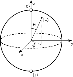
Figure 1: Bloch sphere

Hilbert spaces and composite systems

The state vector of a quantum system is defined in a complex vector space called Hilbert space $\mathcal{H}$. Quantum states are represented in common Dirac notation as “ket’s”, written as the right part $\left|\psi\right\rangle$ of a bracket (“bra-ket”). Algebraically a “ket” is column vector in our state space. This leaves us to define the set of “bra’s” $\langle\phi|$ on the dual space of $\mathcal{H}$, $\mathcal{H^{\star}}$. The dual Hilbert space $\mathcal{H^{\star}}$ is defined as the set of linear maps $\mathcal{H}\rightarrow\textbf{C}$, given by

$$\langle\phi|\>:\,\left|\psi\right\rangle\mapsto\langle\phi|\psi\rangle\in\textbf{C},$$ (6)

where $\langle\phi|\psi\rangle$ is the inner product of the vectors $\left|\psi\right\rangle,\left|\phi\right\rangle\in\mathcal{H}$. We can now write down a more formal definition of a Hilbert space: It is a complex inner product space with the following properties:

1. $\langle\phi|\psi\rangle=\langle\psi|\phi\rangle^{\dagger}$, where $\langle\psi|\phi\rangle^{\dagger}$ is the complex conjugate of $\langle\psi|\phi\rangle$.

2. The inner product$\langle\phi|\psi\rangle$ is linear in the first argument: $\langle a\phi_{1}+b\phi_{2}|\psi\rangle=a^{\dagger}\langle\phi_{1}|\psi\rangle+b^{\dagger}\langle\phi_{2}|\psi\rangle$.

3. $\langle\psi|\psi\rangle\geq 0$.

The space of a $n$ qubit system is spanned by a basis of $2^{n}$ orthogonal vectors $\left|e_{i}\right\rangle$; one for each possible combination of the basis-states of the individual qubits, obeying the orthogonality condition:

$$\langle e_{i}|e_{j}\rangle=\delta_{ij},$$ (7)

where $\delta_{ij}=1$ for $i=j$ and $\delta_{ij}=0$ for $i\neq j$. We say that the Hilbert space of a composite system is the tensor products of the Hilbert spaces of its parts. So the space of a $n$ qubit system is simply the tensor product of the spaces of the $n$ qubits.

$$\mathcal{H}_{\mathcal{Q}}=\mathcal{H}_{\mathcal{Q}_{n}}\otimes\mathcal{H}_{\mathcal{Q}_{n}-1}\otimes\mathcal{H}_{\mathcal{Q}_{n-2}}...\otimes\mathcal{H}_{\mathcal{Q}_{1}},$$ (8)

where $\mathcal{Q}_{i}$ the quantum system $i$ is a vector in $\textbf{C}^{2}$. A general $n$ qubit system can therefore be written

$$\left|\psi\right\rangle=\sum_{x_{n},..,x_{1}=0}^{1}a_{x_{n}...x_{1}}\left|x_{n}\cdots x_{1}\right\rangle,$$ (9)

where

$$\left|x_{n}\cdots x_{1}\right\rangle=\left|x_{n}\right\rangle\otimes\left|x_{n-1}\right\rangle\otimes\cdots\otimes\left|x_{1}\right\rangle\in\mathcal{H}_{\mathcal{Q}}$$ (10)

with $x_{i}\in\{0,1\}$ and complex coefficients $a_{x_{i}}$. For a two qubit system, $\left|x_{2}\right\rangle\otimes\left|x_{1}\right\rangle=\left|x_{2}\right\rangle\left|x_{1}\right\rangle=\left|x_{2}x_{1}\right\rangle$, we have

$$\left|\psi\right\rangle=\sum_{x_{2},x_{1}=0}^{1}a_{x_{2}x_{1}}\left|x_{2}x_{1}\right\rangle=a_{00}\left|00\right\rangle+a_{01}\left|01\right\rangle+a_{10}\left|10\right\rangle+a_{11}\left|11\right\rangle$$ (11)

This state space is therefore spanned by four basis vectors:

$$\left|00\right\rangle,\left|01\right\rangle,\left|10\right\rangle,\left|11\right\rangle,$$ (12)

which are represented by the following 4-dimensional column vectors respectively:

$$\left(\begin{array}[]{c}1\\ 0\\ 0\\ 0\end{array}\right),\left(\begin{array}[]{c}0\\ 1\\ 0\\ 0\end{array}\right),\left(\begin{array}[]{c}0\\ 0\\ 1\\ 0\end{array}\right),\left(\begin{array}[]{c}0\\ 0\\ 0\\ 1\end{array}\right).$$ (13)

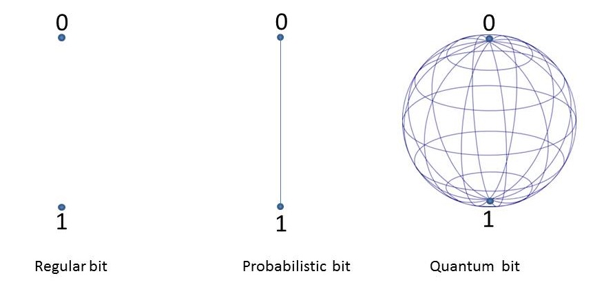
Figure 2: The classical bit has only two distinct states, the probabilistic bit can be in any normalized convex combination of those states, whereas the quantum bit has a much richer state space.

Operators

A linear operator on a vector space $\mathcal{H}$ is a linear transformation $\mathrm{T\,}:\mathcal{\>H}\rightarrow\mathcal{H}$, that maps vectors in $\mathcal{H}$ to vectors in the same space $\mathcal{H}$. Quantum states are normalized, and we wish to keep the normalization; we are therefore interested in transformations that can be regarded as rotations in $\mathcal{H}$. Such transformations are given by unitary operators $U$. An operator $U$ is called unitary if $U^{-1}=U^{\dagger}$. They preserve inner products between vectors, and thereby their norm. A projection operator $P$ is Hermitian i.e. $P=P^{\dagger}$ and satisfies $P^{2}=P$. We can create a projector $P$, by taking the outer product of a vector with itself:

$$P=\left|\phi\right\rangle\langle\phi|.$$ (14)

$P$ is a matrix with every element $P_{ij}$ being the product of the elements $i,j$ of the vectors in the outer product. This operator projects any vector $\left|\gamma\right\rangle$ onto the 1-dimensional subspace of $\mathcal{H}$, spanned by $\left|\phi\right\rangle$:

$$P\left|\gamma\right\rangle=\left|\phi\right\rangle\langle\phi|\left|\gamma\right\rangle=\langle\phi|\gamma\rangle\left|\phi\right\rangle.$$ (15)

It simply gives the portion of $\left|\gamma\right\rangle$ along $\left|\phi\right\rangle$.
We will often deal with unitary operators $U\in\mathrm{SU(2)}$, i.e operators from the special unitary group of dimension 2. The group consists of $2\times 2$ unitary matrices with determinant 1. These matrices will be operating on single qubits (often in systems of 2 or more qubits). The generators of the group are the Pauli spin matrices $\sigma_{x},\,\sigma_{y},\,\sigma_{z}$, shown together with the identity matrix $I$:

$$I=\left(\begin{array}[]{cc}1&0\\ 0&1\end{array}\right),\;\sigma_{x}=\left(\begin{array}[]{cc}0&1\\ 1&0\end{array}\right),\;\sigma_{y}=\left(\begin{array}[]{cc}0&-i\\ i&0\end{array}\right),\;\sigma_{z}=\left(\begin{array}[]{cc}1&0\\ 0&-1\end{array}\right).$$ (16)

Note that $\sigma_{x}$ is identical to a classical (bit-flip) ’NOT’-operation. General $2\times 2$ unitary operators can be parameterized with three parameters $\theta,\alpha,\beta$, as follows:

$$U\left(\theta,\alpha,\beta\right)=\left(\begin{array}[]{cc}e^{i\alpha}\cos\left(\theta/2\right)&ie^{i\beta}\sin\left(\theta/2\right)\\ ie^{-i\beta}\sin\left(\theta/2\right)&e^{-i\alpha}\cos\left(\theta/2\right)\end{array}\right).$$ (17)

An operation is said to be local if it only affects a part of a composite (multi-qubit) system. Connecting this to the concept of the bit-strings in the previous section; a local operation translates to just controlling one such bit. This is a crucial point in the case of modeling the effect of individual actions, since each agent in a strategic situation is naturally constrained to decisions regarding their own choices. The action of a set of local operations on a composite system is given by the tensor product of the local operators. For a general n-qubit $\left|\psi\right\rangle$ as given in (9) and (10) we get:

$$U_{n}\otimes U_{n-1}\otimes\cdots\otimes U_{1}\left|\psi\right\rangle=\sum_{x_{n},..,x_{1}=0}^{1}a_{x_{n}...x_{1}}U_{n}\left|x_{n}\right\rangle\otimes U_{n-1}\left|x_{n-1}\right\rangle\otimes\cdots\otimes U_{1}\left|x_{1}\right\rangle.$$ (18)

Mixed states and the density operator

We have so far only discussed pure states, but sometimes we encounter quantum states without a definite state vector $\left|\psi\right\rangle$, these are called mixed states and consists of a states that has certain probabilities of being in some number of different pure states. So for example a state that is in $\left|\psi_{1}\right\rangle=a_{0}^{1}\left|0\right\rangle+a_{1}^{1}\left|1\right\rangle$ with probability $p_{1}$ and in $\left|\psi_{2}\right\rangle=a_{0}^{2}\left|0\right\rangle+a_{1}^{2}\left|1\right\rangle$ with probability $p_{2}$ is mixed. We handle mixed states by defining a density operator $\rho$, which is a hermitian matrix with unit trace:

$$\rho=\sum_{i}p_{i}\left|\psi_{i}\right\rangle\langle\psi_{i}|,$$ (19)

where $\sum_{i}p_{i}=1$. A pure state in this representation is simply a state for which all probabilities, except one is zero. If we apply a unitary operator $U$ on a pure state, we end up with $U\left|\psi\right\rangle$ which has the density operator $U\rho U^{\dagger}=U\left|\psi\right\rangle\langle\psi|U^{\dagger}$. Regardless if we are dealing with pure or mixed states, we take the expectation value of upon measurement ending up in a $\left|\phi\right\rangle$ by calculating $\mathrm{Tr}\left(\left|\phi\right\rangle\langle\phi|\rho\right)$, where $|\phi\rangle\langle\phi|$ is a so called projector. For calculating the expectation values of a state to be in any of a number of states $|\phi_{i}\rangle$, we construct a projection operator $P=\sum_{i}|\phi_{i}\rangle\langle\phi_{i}|$ and take the trace over $P$ multiplied by $\rho$.

Entanglement

Entanglement is the resource our game-playing agents will make use of in the quantum game protocols to achieve better than classical performance. Non-classical correlations are thus introduced, by which the players can synchronize their behavior without any additional communication. An entangled state is basically a quantum system that cannot be written as a tensor product of its subsystems, we’ll thus define two classes of quantum states. Examples below refers to two-qubit states.

Product states:

$$|\Psi_{\mathcal{Q}}\rangle=|\Psi_{\mathcal{Q}_{2}}\rangle\otimes|\Psi_{\mathcal{Q}_{1}}\rangle,~{}~{}\textrm{or using density matrix}~{}~{}\rho_{\mathcal{Q}}=\rho_{\mathcal{Q}_{2}}\otimes\rho_{\mathcal{Q}_{1}},$$ (20)

and entangled states

$$|\Psi_{\mathcal{Q}}\rangle\neq|\Psi_{\mathcal{Q}_{2}}\rangle\otimes|\Psi_{\mathcal{Q}_{1}}\rangle,~{}~{}\textrm{or using density matrix }~{}~{}\rho_{\mathcal{Q}}\neq\rho_{\mathcal{Q}_{2}}\otimes\rho_{\mathcal{Q}_{1}}.$$ (21)

For a mixed state, the density matrix is defined as mentioned by $\rho_{\mathcal{Q}}=\sum^{N}_{i=1}p_{i}|\psi_{i}\rangle\langle\psi_{i}|$ and it is said to be separable, which we will denote by $\rho^{sep}_{\mathcal{Q}}$, if it can be written as

$$\rho^{sep}_{\mathcal{Q}}=\sum_{i}p_{i}(\rho^{i}_{\mathcal{Q}_{2}}\otimes\rho^{i}_{\mathcal{Q}_{1}}),~{}\sum_{i}p_{i}=1.$$ (22)

A set of very important two-qubit entangled states are the Bell states

$$|\Phi^{\pm}_{\mathcal{Q}}\rangle=\frac{1}{\sqrt{2}}(|{00}\rangle\pm|11\rangle),~{}~{}~{}~{}|\Psi^{\pm}_{\mathcal{Q}}\rangle=\frac{1}{\sqrt{2}}(|{01}\rangle\pm|10\rangle).$$ (23)

The GHZ-type-states

$$|\textrm{GHZ}_{n}\rangle=\frac{1}{\sqrt{2}}\left(|00\cdots 0\rangle+e^{i\phi}|11\cdots 1\rangle\right)$$ (24)

could be seen as a $n$-qubit generalization of $|\Phi^{\pm}_{\mathcal{Q}}\rangle$-states.

1.3 Classical Games

It is instructive to review the theory of classical games and some major solution concepts before moving on to examples of quantum games. We’ll start by defining classical pure and mixed strategy games, and then move on to introducing some relevant solution concepts and finish off with a definition of quantum games.

A game is a formal model over the interactions between a number of agents (agents, players, participants, and decision makers may be used interchangeably) under some specified sets of choices (choices, strategies, actions and moves, may be used interchangeably). Each combination of choices made, or strategies chosen by the different players leads to an outcome with some certain level of desirability for each of them. The level of desirability is measured by assigning a real number, a so called payoff $\$$ for each game outcome for each player. Assuming rational players, each will choose actions that maximizes their expected payoff $E(\$)$, i.e. in an deterministic as well as in an probabilistic setting acting in a way that, based on the known information about the situation, maximizes the expectation value of their payoff. The structure of the game is fully specified by the relations between the different combinations of strategies and the payoffs received by the players. A key point is the interdependence of the payoffs with the strategies chosen by the other players. A situation where the payoff of one player is independent of the strategies of the others would be of little interest from a game theoretical point of view. It is natural to extend the notion of payoffs to payoff functions whose arguments are the chosen strategies of all players and ranges are the real valued outputs that assigns a level of desirability for each player to each outcome.

Pure strategy classical game

We have a set of $n$ players $\{1,2,...,n\}$, $n$ strategy sets $S_{i}$, one for each player $i$, with $s_{i}^{j}\in S_{i}$, where $s_{i}^{j}$ is the $j$:th strategy of player $i$. The strategy space $S=S_{1}\times S_{2}\times\cdots\times S_{n}$ contains all $n$-tuples pure strategies, one from each set. The elements $\sigma\in S$ are called strategy profiles, some of which will earn them the status of being a solution with regards to some solution concept.

We define a game by its payoff-functions $\$_{i}$, where each is a mapping from the strategy space $S$ to a real number, the payoff or utility of player $i$. We have:

$$\$_{i}:S_{1}\times S_{2}\times\cdots\times S_{n}\rightarrow\textbf{R}.$$ (25)

Mixed strategy classical game

Let $\Delta(S_{i})$ be the set of convex linear combinations of the elements $s_{i}^{j}\in S_{i}$. A mixed strategy $s^{mix}_{i}\in\Delta(S_{i})$ is then given by:

$$\sum_{s^{j}_{i}\in S_{i}}p_{i}^{j}s^{j}_{i}\;\;\;\textrm{with}\;\;\;\sum_{j}p_{i}^{j}=1,$$ (26)

where $p^{j}_{i}$ is the probability player $i$ assigns to the choice $s^{j}_{i}$. The space of mixed strategies $\Delta(S)=\Delta(S_{1})\times\Delta(S_{2})\times\cdots\times\Delta(S_{n})$ contains all possible mixed strategy profiles $\sigma_{mix}$. We now have:

$$\$_{i}:\Delta(S_{1})\times\Delta(S_{2})\times\cdots\times\Delta(S_{n})\rightarrow\textbf{R}.$$ (27)

Note that the pure strategy games are fully confined within the definition of mixed strategy games and can be accessed by assigning all strategies except one, the probability $p^{j}=0$. This class of games could be formalized in a framework using probabilistic information units, such as the probabilistic bit.

1.4 Solution concepts

We will introduce two of many game theoretical solution concepts. A solution concept is a strategy profile $\sigma^{*}\in S$, that has some particular properties of strategic interest. It could be a strategy profile that one would expect a group of rational self-maximizing agents to arrive at in their attempt to maximize their minimum expected payoff. Strategy profiles of this form i.e. those that leads to a combination of choices where each choice is the best possible response to any possible choice made by other players tend to lead to an equilibrium, and are good predictors of game outcomes in strategic situations. To see how such equilibria can occur we’ll need to develop the concept of dominant strategies.

Definition 1

(Strategic dominance): A strategy $s^{dom}\in S_{i}$ is said to be dominant for player $i$, if for any strategy profile $\sigma_{-i}\in S/S_{i}$, and any other strategy $s^{j}\neq s^{dom}\in S_{i}$:

$$\$_{i}(s^{dom},\sigma_{-i})\geq\$_{i}(s^{j},\sigma_{-i})\;\;\textrm{for all}\;\;i=1,2,\cdots,n.$$ (28)

Lets look at a simple example. Say that we have two players, Alice with legal strategies $s^{1}_{Alice},s^{2}_{Alice}\in S_{Alice}$ and Bob with $s^{1}_{Bob},s^{2}_{Bob}\in S_{Bob}$. Now, if the payoff Alice receives when playing $s^{1}_{Alice}$ against any of Bob’s two strategies is higher than (or at least as high as) what she receives by playing $s^{2}_{Alice}$, then $s^{1}_{Alice}$ is her dominant strategy. Her payoff can of course vary depending on Bob’s move but regardless what Bob does, her dominant strategy is the best response. Now there is no guarantee that such dominant strategy exists in a pure strategy game, and often must the strategy space be expanded to accommodate for mixed strategies for them to exist.

If both Alice and Bob has a dominant strategy, then this strategy profile becomes a Nash Equilibrium, i.e. a combination of strategies for which none of them can gain by unilaterally deviating from. The Nash equilibrium profile acts as an attractor in the strategy space and forces the players into it, even though it is not always an optimal solution. Combinations can exist that can lead to better outcomes for both (all) players.