Herschel far-infrared observations of the Carina Nebula complex

Abstract

Context. The Carina Nebula represents one of the most massive star forming regions known in our Galaxy and displays a high level of feedback from the large number of very massive stars. While the stellar content is now well known from recent deep X-ray and near-infrared surveys, the properties of the clouds remained rather poorly studied until today.

Aims. By mapping the Carina Nebula complex in the far-infrared, we aim at a comprehensive and detailed characterization of the dust and gas clouds in the complex.

Methods. We used SPIRE and PACS onboard of Herschel to map the full spatial extent ($\approx 5.3$ square-degrees) of the clouds in the Carina Nebula complex at wavelengths between $70\,\mu$m and $500\,\mu$m. We use here the $70\,\mu$m and $160\,\mu$m far-infrared maps to determine color temperatures and column densities, and to investigate the global properties of the gas and dust clouds in the complex.

Results. Our Herschel maps show the far-infrared morphology of the clouds at unprecedented high angular resolution. The clouds show a very complex and filamentary structure that is dominated by the radiation and wind feedback from the massive stars. In most locations, the column density of the clouds is $N_{\rm H}\la 2\times 10^{22}\,\rm cm^{-2}$ (corresponding to visual extinctions of $A_{V}\la 10$ mag); denser cloud structures are restricted to the massive cloud west of Tr 14 and the innermost parts of large pillars. Our temperature map shows a clear large scale gradient from $\approx 35-40$ K in the central region to $\la 20$ K at the periphery and in the densest parts of individual pillars. The total mass of the clouds seen by Herschel in the central (1 degree radius) region is $\approx 656\,000\,M_{\odot}$. We also derive the global spectral energy distribution in the mid-infrared to mm wavelength range. A simple radiative transfer model suggests that the total mass of all the gas (including a warmer component that is not well traced by Herschel) in the central 1 degree radius region is $\leq 890\,000\,M_{\odot}$.

Conclusions. Despite the strong feedback from numerous massive stars and the corresponding cloud dispersal processes that are going on since several million years, there are still several $10\,000\,M_{\odot}$ of cool cloud material present at column-densities sufficient for further star formation. Comparison of our total gas mass estimates to molecular cloud masses derived from CO line mapping suggests that as much as about 75% of all the gas is in atomic rather than molecular form.

1 Introduction

Most stars form in large clusters or associations, containing (at least) several thousand stars (e.g., Briceño et al. 2007), and it has recently become clear that also our sun formed as part of a large star forming complex (e.g., Adams 2010). In contrast to low-mass star forming regions like Taurus, where the individual young stellar objects (YSOs) form more or less in isolation and any interaction is minimal, large clusters and associations contain high-mass ($M\geq 20\,M_{\odot}$) stars. These hot and luminous O-type stars profoundly influence their environments (see, e.g. Freyer et al. 2003) by creating HII regions, generating wind-blown bubbles, and exploding as supernovae. This feedback can disperse the natal molecular clouds and thus halt further star formation. However, advancing ionization fronts and expanding superbubbles can also compress nearby clouds and thereby trigger the formation of new generations of stars (e.g., Reach et al. 2004; Cannon et al. 2005; Oey et al. 2005; Preibisch & Zinnecker 2007; Deharveng et al. 2009; Zavagno et al. 2010; Brand et al. 2011). The interaction of the massive stars with the surrounding clouds and the balance between cloud destruction and triggered star formation determine the characteristics and the final outcome of the star formation process (see Dale et al. 2007; Dale & Bonnell 2008; Bate 2009; Gritschneder et al. 2010, for numerical studies).

At a distance of 2.3 kpc, the Carina Nebula Complex (CNC, hereafter; see Smith & Brooks 2008, for a recent review) is the nearest star forming region with a large population of very massive stars (at least 70 O-type and WR stars; see Smith 2006). Among these are several of the most massive ($M\ga 100\,M_{\odot}$) and luminous stars known in our Galaxy, e.g., the famous Luminous Blue Variable $\eta$ Car, the O2 If* star HD 93129Aa, several O3 main sequence stars, and four Wolf-Rayet stars. Most of the massive stars reside in several loose clusters near the center of the complex, including Tr 14, 15, and 16, which have ages ranging from $<$1 to $\sim 8$ Myr (see Dias et al. 2002; Preibisch et al. 2011c). The CNC contains large amounts of gas and dust clouds, with an estimated total mass in the range $350\,000-670\,000\,M_{\odot}$ based on CO radio maps (e.g. Grabelsky et al. 1988; Yonekura et al. 2005; Smith & Brooks 2007). The very strong radiative and wind feedback from the massive stars has already dispersed much of the original cloud mass in the central region, and drives a large expanding superbubble, extending over $\sim 80$ pc (corresponding to $\sim 2\degr$).

During the last few years, several surveys have provided a wealth of new information on the stellar populations in the CNC. The HST survey of the central area (Smith et al. 2010a) and a Spitzer survey of the southern parts of the CNC (Smith et al. 2010b) showed that the ionizing radiation from the massive stars is currently triggering the formation of a new generation of stars in the remaining dense clouds, in particular in the so-called “Southern Pillars” region.

We have performed a very deep near-infrared survey of the central $\sim 1300$ square-arcminute area of the CNC with the near-infrared camera HAWK-I at the ESO 8m-VLT (Preibisch et al. 2011c) which is deep enough to reveal all young stars in the region with $A_{V}\leq 35$ mag.

The Chandra Carina Complex Project (see Townsley et al. 2011, for an overview) has mapped the CNC with a mosaic of 22 individual ACIS-I pointings, using a total observing time of 1.34 Megaseconds (15.5 days) and covering an area of about 1.4 square-degrees. With the detection of more than 11 000 X-ray emitting young stars, these Chandra data efficiently eliminate the strong field-star confusion problems that plague visual and IR samples and provide, for the first time, a large sample of the young stellar population (down to $\sim 0.5\,M_{\odot}$) in the area. A detailed statistical analysis of the X-ray, optical, and infrared properties of the detected sources showed that 10 714 of the X-ray sources are very likely young stars in the CNC (Broos et al. 2011b). The analysis of the spatial distribution of the X-ray detected young stars showed that half of the young stellar population resides in one of about 30 clusters or stellar groups, while the other half constitutes a widely dispersed population (Feigelson et al. 2011). The combination of the X-ray data with near- and mid-infrared photometry provided new information about the properties of the stellar populations in the entire complex (Povich et al. 2011; Preibisch et al. 2011b) and the individual clusters Tr 14 and Tr 15 (Wolk et al. 2011; Wang et al. 2011). These studies showed that the X-ray detected young stellar populations have ages ranging from $<1$ Myr up to $\approx 8$ Myr, and support the scenario of ongoing, triggered star formation in the CNC.

While these new data sets have strongly boosted the amount of available information about the stellar populations, the knowledge about the clouds in the complex is still much more limited. While the IRAS maps and several existing radio maps of CO and other molecular lines provide basic information on the large-scale morphology of the clouds, only very small areas at the center of the complex have been observed with sub-arcminute angular resolution at far-infrared (FIR) and (sub)-mm wavelengths so far (Brooks et al. 2005; Gomez et al. 2010). This lack of sensitive FIR and (sub)-mm data with sufficient spatial resolution strongly hampers studies of the cloud structure, and is a very serious obstacle for investigations of global cloud properties and the interaction between massive stars and clouds in the CNC.

As a first step to improve this situation, we have recently used LABOCA at the APEX telescope to obtain a sensitive wide-field ($1.25\hbox{${}^{\circ}$}\times 1.25\hbox{${}^{\circ}$}$) sub-mm map of the CNC at a wavelength of $870\,\mu$m with $18^{\prime\prime}$ angular resolution ($=$ 0.2 pc at the distance of the CNC), which provides the first large-scale survey of the dusty clouds in this region (Preibisch et al. 2011a). These data showed that there are (at least) $\sim 60\,000\,M_{\odot}$ of dust and gas in dense, compact clouds; this represents a large potential for further star formation. While this LABOCA map provided important information about the global properties of the dense clouds in the complex, the information that can be retrieved about the total cloud phase is limited by two factors: First, the LABOCA map is only sensitive to the dense, localized clouds. As a consequence of the removal of correlated noise in the data reduction, structures with angular sizes larger $\approx 2.5^{\prime}$ are only partly recovered. Therefore, the more diffuse emission from less dense gas is missing from the map. The second limitation is that a single-wavelength band map does not allow the determination of cloud temperatures. This is critical, because information on the cloud temperature is required to compute reliable cloud masses from the observed fluxes. The often used approach of simply assuming a uniform “typical” cloud temperature (e.g., 15 K) is very likely not appropriate in the case of the CNC, where some clouds are very strongly irradiated (and thus heated) by numerous nearby massive stars, while other clouds (especially at the periphery of the CNC) experience orders of magnitudes lower levels of irradiation (and correspondingly less heating from outside). FIR maps at several different wavelengths can provide crucial information about the cloud temperatures and thus allow much more reliable mass and column-density estimates than based on single-wavelength data.

In the present paper we will be discussing observations of the CNC performed with the ESA Herschel Space Observatory (Pilbratt et al. 2010), in particular employing Herschel’s large telescope and powerful science payload to do photometry using the PACS (Poglitsch et al. 2010) and SPIRE (Griffin et al. 2010) instruments. We will present an overview of the project, determine color temperature and column density maps and investigate the statistics of these quantities in selected regions of our maps. We also investigate global properties of the CNC clouds derived from our results.

2 Herschel far-infrared mapping of the Carina Nebula

In the Herschel open time project OT1_tpreibis_1 we used PACS and SPIRE to map the entire extent of the CNC in five bands between $70\,\mu$m and $500\,\mu$m. The observation was performed on 26 December 2010 in the SPIRE PACS Parallel Mode and used 6.9 hours observing time. The J2000 coordinates of the aimpoint are RA = 10h44m03s, Dec = -59d30m00s. The fast scan speed (60 arcsec per second) was used to map a $\approx 2.3^{\circ}\times 2.3^{\circ}$ area, which corresponds to a physical region of $\approx 92\,\rm pc\times 92\,pc$ at the distance of the CNC and covers the full spatial extent of the CNC. The mapped area also includes the HII region Gum 31 (= Ced 108 = NGC 2599; see Cederblad 1946; Gum 1955) around the young stellar cluster NGC 3324 at the north-western edge of the Carina Nebula.

The observation was done with two scan maps of the same area, one with nominal scan direction, and the other with orthogonal scan direction, in order to remove more efficiently the stripping effects due to the $1/f$ noise and to get better coverage redundancy.

We used the $70\,\mu$m PACS channel as the blue band, in order to get the widest possible wavelength range. The wavelength bands of the five maps resulting from our observations are $[60-85]\,\mu$m, $[130-210]\,\mu$m, $[210-290]\,\mu$m, $[300-400]\,\mu$m, and $[420-610]\,\mu$m, and will be denoted as the $70\,\mu$m, $160\,\mu$m, $250\,\mu$m, $350\,\mu$m, and $500\,\mu$m band in the following text.

The data reduction was performed with the HIPE v7.0 (Ott 2010) and SCANAMORPHOS v10.0 (Roussel 2012) software packages. From level 0.5 to 1 the PACS data was reduced using the L1_scanMapMadMap script in the photometry pipeline in HIPE with the version 32 calibration tree. The level 2 maps were produced with SCANAMORPHOS with standard options for parallel mode observations and the galactic option to preserve brightness gradients over the field. The pixel sizes of the two PACS maps were chosen as $3.2\arcsec$ (for the $70\,\mu$m map) and $4.5\arcsec$ (for the $160\,\mu$m map), as suggested in Traficante et al. (2011).

The level 0 SPIRE data were reduced with an adapted version of the HIPE script rosette_obsid1&2_script_level1 included in the SCANAMORPHOS package. The final maps were produced by SCANAMORPHOS with standard options for parallel mode observations and the galactic option as for the PACS data. The pixel sizes were chosen as $6\arcsec$, $8\arcsec$ and $11.5\arcsec$, for the 250, 350, and 500 $\mu$m band, respectively.

The quality of the final maps turned out to be very good. In order to characterize the point-spread-function (PSF) in the maps, we determined the full-width at half-maximum (FWHM) for a number of isolated point-like sources and found values of $\approx 10^{\prime\prime}$ for the $70\,\mu$m map, $\approx 15^{\prime\prime}$ for the $160\,\mu$m map, $\approx 20^{\prime\prime}$ for the $250\,\mu$m map, $\approx 26^{\prime\prime}$ for the $350\,\mu$m map, and $\approx 36^{\prime\prime}$ for the $500\,\mu$m map. These values show that the image quality of the PACS maps is slightly worse than the telescope diffraction limit (as expected for observations performed in fast scan mode), but the SPIRE maps are close to the ideal quality. With their unprecedented angular resolution of $\sim 10^{\prime\prime}-36^{\prime\prime}$, corresponding to physical scales of $\sim 0.1-0.4$ pc, these Herschel maps represent the first detailed, deep, and spatially complete FIR maps of the full CNC.

The levels of background cloud fluctuations, determined as the standard deviation of the pixel value in apparently empty regions in the maps, are found to be $\approx 2.3$ mJy/px at $70\,\mu$m, $\approx 5.0$ mJy/px at $160\,\mu$m, $\approx 84$ mJy/beam at $250\,\mu$m, $\approx 83$ mJy/beam at $350\,\mu$m, and $\approx 73$ mJy/beam at $500\,\mu$m.

A potential problem in the calibration of the Herschel maps is the possible presence of zero-level offsets (see Bernard et al. 2010). No correction for these offsets is currently implemented in the Herschel data reduction tools. There are several reasons why we can expect the uncertainties related to offsets to be only moderate for our specific data set and the results obtained in this paper. One reason is that by the use of the the galactic option in SCANAMORPHOS the baseline subtraction is modified with the aim to preserve large-scale structures as well as possible. Another important aspect is that our maps cover the entire spatial extent of the clouds associated with the Carina Nebula. The periphery of our maps shows low-intensity galactic background emission that is not related to the Carina Nebula and thus not relevant for the aims of our study. Therefore, the emission from the relevant clouds associated to the Carina Nebula can be well separated from the galactic background in our maps. We also compared our Herschel $70\,\mu$m map to the IRAS $60\,\mu$m map and found very good agreement (within about 1%) of the fluxes integrated over large regions. Finally, we note that in our temperature and column density determination described in the next section even a 20% error in the intensity causes just a $\sim 5\%$ change in the derived color temperatures and a $\sim 12\%$ change in the derived cloud column densities.

As soon as the Planck data get available, a more detailed analysis of the possible effects of offset corrections will be performed.

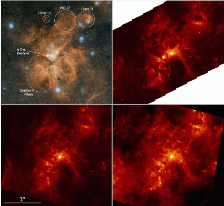
Figure 1: Optical, near-, and far-infrared view of the Carina Nebula. All four images show the same field of view of $3\degr\times 3\degr$. North is up and east to the left. Upper left: Optical image obtained from the ESO Photo Release 1145 (http://www.eso.org/public/images/eso0905b/; ESO/Digitized Sky Survey 2, Davide De Martin). Upper right: $5.8\,\mu$m image constructed by us from Spitzer data obtained from the public archive. Lower left: Herschel $70\,\mu$m map. Lower right: Herschel $500\,\mu$m map. The Spitzer and Herschel images are displayed with a square-root intensity scale.

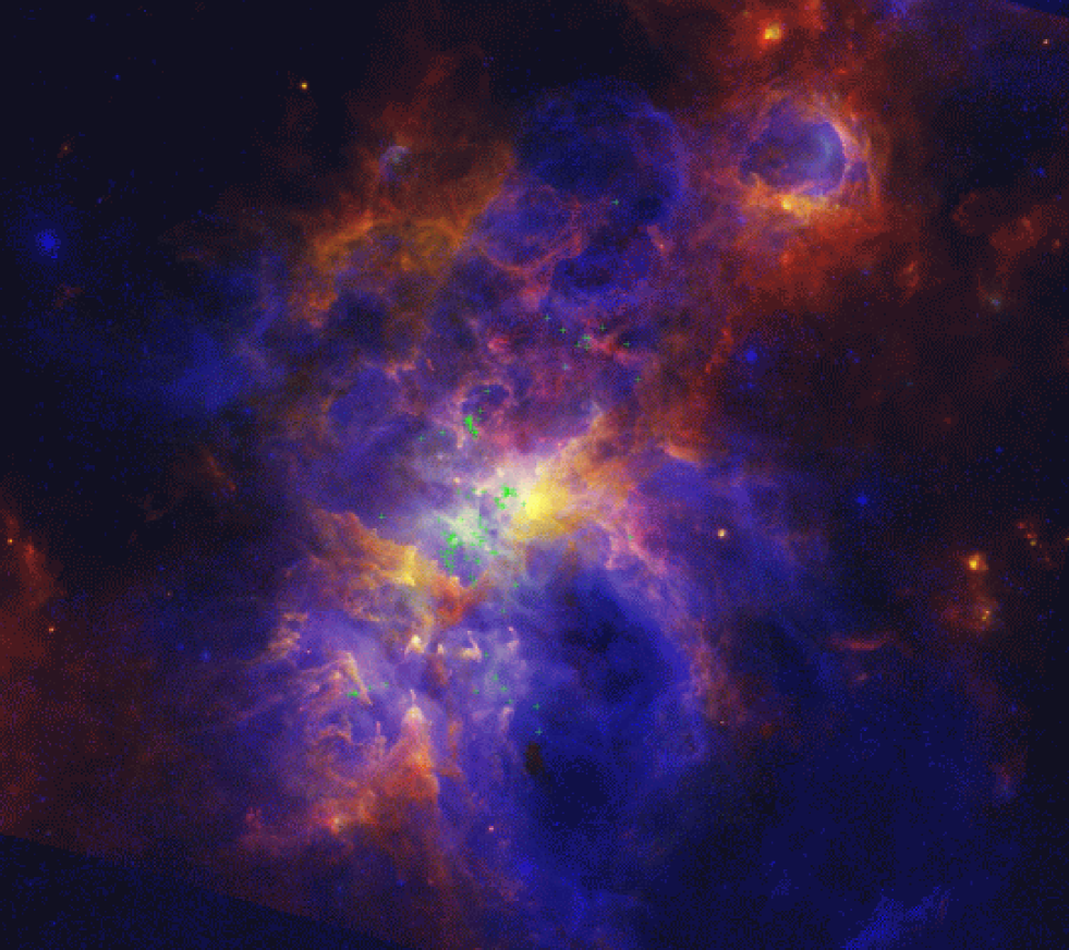
Figure 2: RGB composite of the red optical (DSS) image in blue, the Herschel $70\,\mu$m image in green, and the Herschel $160\,\mu$m image in red. The image shows a $2.9\degr\times 2.6\degr$ field of view. North is up and east to the left. The green plus signs mark the positions of the high-mass stellar members of the CNC as listed in Smith (2006).

3 Cloud morphology

The complete set of all five Herschel maps resulting from our observation is shown in Figures A1 to A5 in the appendix. In Figure 1 we compare the $70\,\mu$m and $500\,\mu$m Herschel maps to an optical image and the Spitzer $5.8\,\mu$m image. The remarkable similarity between the Herschel 70 $\mu$m image and the Spitzer $5.8\,\mu$m image demonstrates that most of the clouds are only moderately dense, i.e., are already transparent in the Spitzer $5.8\,\mu$m band. This point will be discussed in more detail in Sect. 5.

In Fig. 2 we show an RGB color composite of the optical, $70\,\mu$m and $160\,\mu$m emission. This illustrates the spatial relation between the hot ($\sim 10^{4}$ K) H$\alpha$ emitting gas and the dense cool/cold gas. It shows how the hot gas fills the interior of the bubbles in the cloud structure.

The comparison of the Herschel  $70\,\mu$m maps to our LABOCA $870\,\mu$m map presented in Preibisch et al. (2011a) shows that the detectable sub-mm emission is restricted to a small volume fraction of the cloud shown by Herschel. The volume filling factor of the dense clouds is very low, and this dense material is highly fragmented and dispersed throughout the area. Herschel reveals the much more widespread diffuse gas at lower densities.

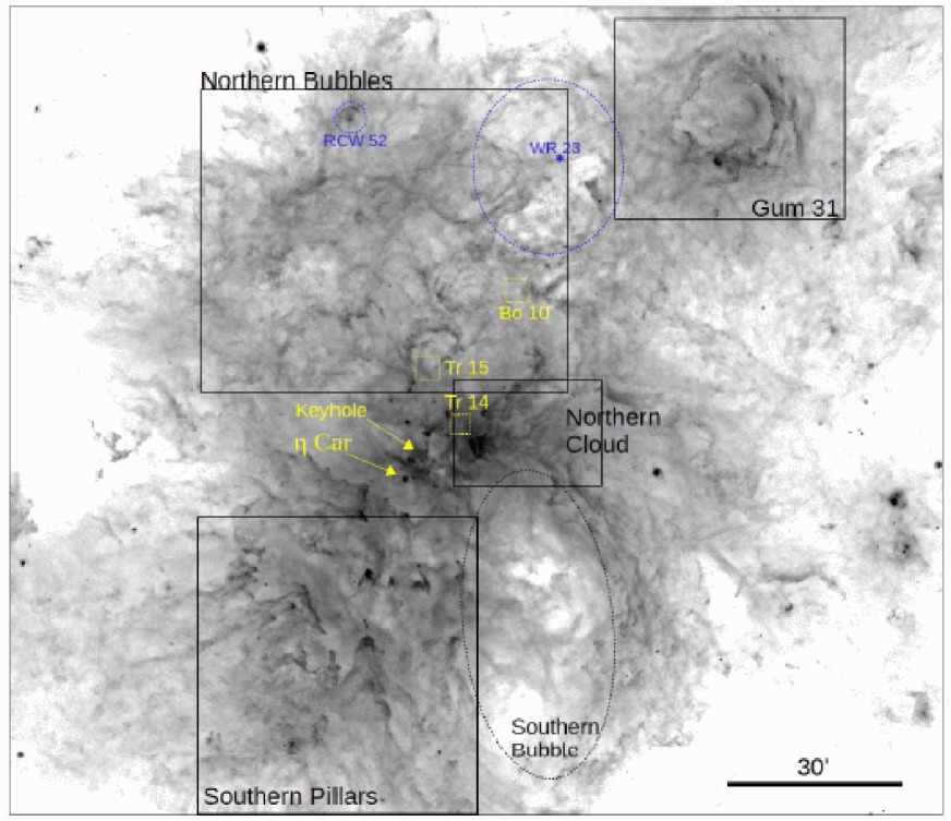
Figure 3: Unsharp-masked version of the Herschel $70\,\mu$m image with a logarithmic intensity scale image. The different regions mentioned in Section 3 are marked by the black boxes. The positions of $\eta$ Car, the clusters Tr 14, Tr 14, and Bo 10, as well as the HII regions around WR 23 and RCW 52 are marked. North is up and east to the left.

Figure 3 is an unsharp-mask filtered version of the $70\,\mu$m map that highlights the small-scale structure of the clouds. It clearly shows that the clouds are highly filamentary and have a very complex morphology. Herschel mapping of other star forming regions has shown that molecular clouds generally exhibit an extensive filamentary structure (e.g. André et al. 2010) and that the typical width of these filaments is of the order of $\sim 0.1$ pc (Arzoumanian et al. 2011). This implies that the width of the individual filaments can be only marginally resolved in our $70\,\mu$m map and remains unresolved in the longer wavelength maps of the CNC.

Based on the observed global cloud morphology, we define several sub-regions of the CNC and discuss them separately.

3.1 Central region

In optical images of the Carina Nebula, the “V”-shaped dark clouds just below $\eta$ Car constitute a very prominent feature. The Herschel image shows that these dark clouds are in fact of only moderate density. As we will find below, their typical visual extinction is just $A_{V}\sim 3-5$ mag.

The nebulosity to the north of $\eta$ Car is the well known “Keyhole Nebula”, which was first described by J. Herschel in 1840 (a reproduction of Herschel’s drawing and a comparison to a modern photograph can be found as Fig. 4 in Smith & Brooks 2008). While this nebula contains large amounts of hot gas, producing copious H$\alpha$ emission, it also contains cold molecular clouds (Cox & Bronfman 1995; Brooks et al. 2005; Gomez et al. 2010; Preibisch et al. 2011a)

To the south of $\eta$ Car, the Herschel image shows a region of low emission. This seems to represent a bubble of lower density, that was probably created by the wind- and radiation-feedback from the numerous very massive stars in the Tr 16 cluster.

3.2 Southern Pillars (SP)

The cloud structure in the so-called “Southern Pillars” (SP) was already discussed in detail by Smith et al. (2010b) on the basis of the Spitzer maps. The cloud morphology we see in our Herschel maps is very similar.

3.3 Northern Cloud (NC)

The cloud to the west of the center, close to the stellar cluster Tr 14, is clearly the densest and most massive cloud structure in the complex. Following Schneider & Brooks (2004), we denote it as the “Northern Cloud” (NC). The eastern edge, where this cloud faces the stellar clusters, is the site of a prominent Photon Dominated Region (PDR), which has been studied in some detail by Brooks et al. (2003) and Kramer et al. (2008). Our Herschel maps show that the cloud extends (at least) about $15^{\prime}$ ($\approx 10$ pc) to the west.

3.4 Bubbles north of $\eta$ Car (NB)

The field north of $\eta$ Car also shows a few prominent pillars, but the general structure is dominated by a web of bubbles and arcs. We will therefore denote this region as the “Northern Bubbles” (NB). The diffuse appearance of the clouds and the lack of sub-mm emission from dense clumps in this region suggests that the density contrast of the clouds is smaller than in the SP region, where numerous dense and massive pillars are present. This morphological differences may indicate that the massive star feedback in this area is different from the strong irradiation that shapes the surfaces of the southern pillars.

The bubble-like structure of the clouds is partly related to individual HII regions that have swept up shells of dense clouds around them. The two most prominent HII regions in this area are the extended nebula surrounding the Wolf-Rayet star WR 23 (=HD 92809; spectral type WC6), and the RCW 52 (=Gum 32) nebula (which is illuminated by the O7V star LSS 1887). Both regions are clearly surrounded by bubbles of gas and dust, which have been interpreted as being mainly created by the action of the stellar winds of the massive stars on their environment (Cappa et al. 2005, 2011).

The irregular filamentary structure could be caused by evolved bubbles that already broke up into pieces. We note that this region contains the cluster Tr 15 and Bo 10, which have estimated ages of $7-8$ Myr (Dias et al. 2002; Preibisch et al. 2011c) and are thus several Myr older than the clusters Tr 14 and Tr 16 in the center of the Carina Nebula. This could suggest that at this older age, the stellar-wind feedback (especially from the evolved massive stars) may play an important role. However, the validity of this interpretation remains unclear, since recent studies suggest that massive star feedback is usually dominated by ionizing radiation (e.g. Martins et al. 2010) and the effects of stellar winds are of secondary importance (e.g. Martins et al. 2012).

3.5 The large southern bubble

In the Spitzer images, the large elongated bubble south-west of $\eta$ Car is a quite prominent hole structure. Our Herschel maps confirm that this structure is truly an almost empty bubble, and not caused by the shadow of a dark cloud. Besides the small dense infrared dark cloud described already in Preibisch et al. (2011a), only very low levels of emission are seen in the inner region of this bubble in the Herschel maps. The Herschel maps suggest that the density increases again at the southern edge, i.e. the bubble wall may be closed at the southern edge. The diameter along the major axis is about $50^{\prime}$, corresponding to a physical length of about 33 pc.

The comparison of our FIR maps to the optical image (Fig. 2) shows that the H$\alpha$ emission is well aligned with the inner edges of the inner cloud surface; as the optical emission is strongest at the edges and lower in the central area, this suggests a shell-like morphology for the hot gas.

The origin of this bubble remains unclear. Our search of the SIMBAD database revealed only three known early-type stars inside this bubble: the O8 star HD 305438, the B1/2 II star HD 92741, and the B2 III star HD 92877. None of these seems to be massive enough to have created this large bubble. One possible explanation is that the hot gas from the winds of the numerous massive stars in the central area is leaking out and filling this bubble. An alternative possibility is that this bubble represents the southern lobe of a large bipolar HII region that is driven by the massive stars in Tr 16.

3.6 The Gum 31 bubble

In the north-western part of our Herschel maps, the prominent circular bubble around the HII region Gum 31, which is produced by the young stellar cluster NGC 3324, is clearly the dominating cloud structure. It represents a nice example of a “perfect bubble” of dense clouds around an HII region (see, e.g., Deharveng et al. 2009, for other examples) that has been swept up by the expansion of the HII region.

It is interesting to note that the Herschel maps show elongated filamentary clouds that seem to connect this bubble to the central regions of the Carina Nebula (see Fig. 2). The idea that the Gum 31 bubble is part of the giant Carina Nebula cloud complex is supported by the available information about the radial velocities of the molecular clouds. According to the CO maps of Yonekura et al. (2005), the clouds surrounding Gum 31 have radial velocities in the range $V_{\rm LSR}=-24\dots-21\,{\rm km\,s^{-1}}$, which is very similar to that of the clouds in the central regions of the Carina Nebula, for which a range of $V_{\rm LSR}=-26\dots-18\,{\rm km\,s^{-1}}$ is found. Another interesting aspect is that the densest and most massive parts of this bubble are found at the south and south-eastern regions of the rim, i.e., just along a line connecting the center of the bubble to the center of the Carina Nebula. This may indicate some kind of interaction between the clouds associated with the Carina Nebula and the Gum 31 bubble. A more comprehensive and detailed investigation of these aspects will be the topic of a forthcoming paper.

4 Cloud colors and temperatures

4.1 Morphology in multi-color FIR images

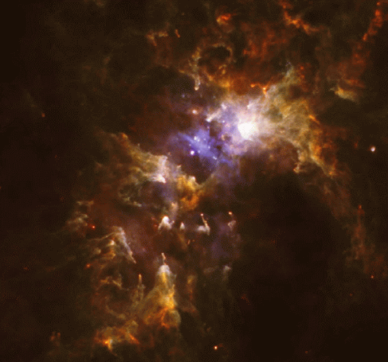
Figure 4: RGB composite of the central region ($1.40\degr\times 1.43\degr$; north is up and east to the left) constructed from our Herschel $70\,\mu$m (blue), $160\,\mu$m (green) and $350\,\mu$m (red).

Figure 4 shows an RGB composite of the central region of the CNC created from our three shortest Herschel wavelengths, in which the colors trace the different cloud temperatures. The bluish emission traces the relatively warm gas in the Keyhole Nebula Region, and also in front of the eastern edge of the Northern Cloud, which is strongly irradiated by the stars in the cluster Tr 14.

The red tones in this image trace the coldest cloud material, which is concentrated in the densest parts of the base of the pillars in the Southern Pillar region, and also in a number of compact clouds north of the Northern cloud.

There are several reddish dense cold clouds to the north-west of center; in contrast to similarly dense clouds in the Southern Pillar region, these do not show a pillar-like structure.

4.2 Color temperatures

In order to estimate the local temperature of the clouds in our map, we determined a color temperature from the ratio of the observed fluxes in two Herschel bands. Due to the high level of radiative feedback from massive stars, which heats the clouds, and the fact that most clouds have only moderate column densities, we can expect that most of the clouds in the CNC should be not extremely cold (such as infrared dark clouds which often show temperatures of $T\leq 15$ K), but somewhat warmer. We will therefore employ the ratio of the $70\,\mu{\rm m}$ versus $160\,\mu{\rm m}$ map intensities, which is well suited to measure temperatures in the range $\sim 20-75$ K. This choice has the advantage that the resulting color temperature maps provide the best angular resolution that can be obtained from our Herschel maps.

In order to construct a flux-ratio map, we first convolved the $70\,\mu$m map with a kernel as discussed in Aniano et al. (2011) to match the angular resolution of the $160\,\mu$m map. Following the procedure for the temperature determinations in the Hi-GAL data described by Bernard et al. (2010), we divided the fluxes derived from the maps by the recommended color-correction factors of 1.05 and 1.29 for the $70\,\mu$m and $160\,\mu$m PACS bands that were derived from a comparison of PACS data to Planck data.

Assuming that we see optically thin thermal dust emission, the ratio of the observed fluxes can be related to the temperature via the formula

$$\frac{I_{\nu}(70\,\mu{\rm m})}{I_{\nu}(160\,\mu{\rm m})}\propto\frac{B_{\nu}(T)(70\,\mu{\rm m})\;\kappa_{\nu}(70\,\mu{\rm m})}{B_{\nu}(T)(160\,\mu{\rm m})\;\kappa_{\nu}(160\,\mu{\rm m})}=f(T)$$ (1)

We further assume that the dust emissivity follows a power-law ($\kappa_{\nu}\propto\nu^{\beta}$). The value of the dust emissivity index $\beta$ is not very well known and under debate; typical observationally determined values range from $\sim 1$ to $\sim 3$, and it is possible that $\beta$ is anti-correlated to the temperature (e.g., Shetty et al. 2009). Here we assume $\beta=2$, what should be appropriate for the relatively warm clouds in the Carina Nebula and has been confirmed for the not too cold ($T\geq 20$ K) clouds in HII regions (see, e.g., Anderson et al. 2010). Equation 1 allows to determine the temperature in each pixel by comparing the observed flux ratio with a pre-computed table of flux-ratio values on a finely space temperature grid.

A complication of this temperature determination method results from the noise in the Herschel maps. In regions with low surface brightness, statistical fluctuations can lead to large errors of the derived temperatures due to division by very small numbers. Furthermore, some outer regions of the maps contain pixels with negative values, preventing any temperature determination. In order to avoid these problems, we restricted the computation of color temperatures to pixels with intensities above the limits of $I_{\nu}(70\,\mu{\rm m})>0.001$ Jy/square-arcsec and $I_{\nu}(160\,\mu{\rm m})>0.01$ Jy/square-arcsec. These limits are several times above the noise-level in the maps and also serve to separate the emission of the clouds in the CNC from the large-scale galactic background emission. This minimum intensity condition is fulfilled for 3 000 757 pixels in our map, i.e. we can derive color temperatures for a total area of about 2.37 square-degrees ($\approx 44\%$ of the full extent of our maps). Since we are only interested here in the properties of the relatively bright clouds associated with the Carina Nebula, these temperature maps cover nevertheless almost the entire area of interest. In the much fainter regions, predominantly around the periphery of our map, for which we cannot determine temperatures, the emission is dominated by the galactic background, which is not of interest for our current study.

A potential problem for the color temperatures may be excess emission from very small dust grains. The absorption of individual optical or UV photons from the surrounding stellar radiation field can cause strong temperature excursions of the smallest grains (with sizes below about 10 nm). Due to these stochastic temperature fluctuations by single-photon heating, the very small grains may not reach an equilibrium temperature. The emission from very small grains in the high-temperature state, immediately after a photon absorption, can lead to an excess of mid-infrared radiation in the total emission spectrum of a cloud with a distribution of grain sizes. As discussed in detail in Draine & Li (2007), two mechanisms play a role. First, photon-heated very small grains consisting of polycyclic aromatic hydrocarbon (PAH) can emit strong mid-infrared band radiation, in particular around the wavelengths of 11.3, 12.7, and $17\,\mu$m. Second, very small carbon and silicate grains may cause an excess of mid-infrared continuum emission. Whereas the Herschel bands do not contain strong PAH emission features, they may be affected by continuum excesses. The strength of excesses from very small grains depends on the ambient radiation field. When the rate of starlight heating is large (as is the case in the Carina Nebula), the relative amplitude of the temperature fluctuations of the grains decreases and the the steady state equilibrium temperature approximation can become valid even for very small grains (see discussion in Sect. 3 of Draine & Li 2007). According to Table 4 in Draine & Li (2007) and in the presence of a radiation field that is 100 times stronger than in the local solar environment, a variation of the abundance of very small grains by a factor of 10 leads to variations in the emissivities of 17% for the $70\,\mu$m PACS band, 7% for the $160\,\mu$m PACS band, and $\leq 5\%$ for the SPIRE bands. We note that a 20% error in the $70\,\mu$m intensity causes a $\sim 5\%$ change in the derived color temperature. This represents a lower limit to the accuracy of the temperature determinations.

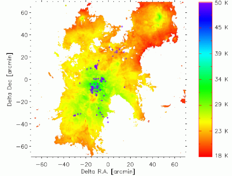
Figure 5: Map of 70–160 $\mu$m color-temperatures. Pixels with insufficient $70\,\mu$m or $160\,\mu$m intensities for a reliable determination of the intensity ratio are left white. The blue plus signs mark the locations of the high-mass stellar members of the CNC as listed in Smith (2006).

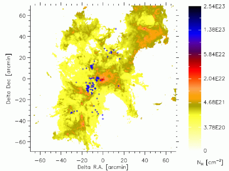
Figure 6: Map of column densities $(N_{\rm H})$ with symbols as in Fig. 5. Pixels with insufficient $70\,\mu$m or $160\,\mu$m intensities for a reliable determination of the intensity ratio are left white.

Figure 5 shows a map of the resulting color temperature values. A histogram of the derived color temperatures can be found in Fig. 7. The color temperatures range from 14 K to 83 K; the mode and the median of the distribution is 29 K and 27.3 K, respectively. Only 4% of the pixels have $T<20\leavevmode\nobreak\ K$, and the fraction of pixels with temperatures of $T>40\leavevmode\nobreak\ K$ [$50\leavevmode\nobreak\ K$] is just 0.39% [0.01%].

In order to estimate the uncertainties of the derived color temperatures, we first note that the flux calibration of the Herschel maps is thought to be accurate to $\sim 10-20\%$; at $T\approx 30$ K, a 20% intensity error causes a 5% ($\approx 1.4$ K) change of the derived color temperature. Besides the above mentioned uncertainties related to possible excess emission from very small grains, another contribution results from the photometric calibration uncertainties of the Herschel bands. For temperatures below $\sim 20$ K, the quickly rising photometric color correction terms cause higher uncertainties and a possible bias towards over-estimated temperatures; however, since only 4% of the pixels in our maps yield such low temperatures, this should not be a serious problem in the analysis of the global properties of the clouds presented in this paper. Furthermore, since our color temperatures are derived from the Herschel maps with the shortest wavelengths, they may be biased towards higher dust temperatures (and consequently lower column densities). Preliminary results from our more detailed investigation (that will be presented in a subsequent publication) suggest that any such bias is rather small. In summary, we estimate the uncertainties of the derived temperatures to be about $\sim 10-15\%$.

We also would like to point out that the temperature values we determined represent averages over the line-of-sight through the full depth of the clouds. Since in some locations there may be several individual clouds that are seen projected onto each other, the physical meaning of the derived temperature is limited, but this is a general problem for the study of cloud properties, and not specific to our data set.

Our temperature map in (Fig. 5) shows a clear systematic temperature gradient from the central regions (where most of the hot, massive stars are located) to the periphery of the complex. A similar, but much steeper temperature gradient is seen within the boundaries of the Gum 31 nebula. This reflects the fact that the number of high-mass stars in NGC 3324 (about 3) is much smaller than the 126 O-, early B-, and WR stars (Smith 2006) in the central regions of the CNC.

5 Cloud column densities

With the temperature estimate we can now proceed and compute the column densities of the clouds. The observed surface brightness in our maps can be converted to the beam-averaged hydrogen column density via the formula

$$N_{\rm H}=2\,N_{\rm H_{2}}=2\,\frac{F_{\nu}\,R}{B_{\nu}(T_{d})\;\Omega\;\kappa_{\nu}\;\mu\,m_{\rm H}}\;\;,$$ (2)

where $\Omega$ is the beam solid angle, $R$ is the gas-to-dust mass ration (assumed here to be 100), $\kappa_{\nu}$ is the dust opacity, and $\mu$ is the mean molecular weight. For consistency with our previous analysis of the LABOCA sub-mm data (Preibisch et al. 2011a), we use the Ossenkopf & Henning (1994) dust model for grains with thin ice-mantles that coagulated at a density of $n=10^{6}\,{\rm cm}^{-3}$ which gives a dust opacity of $\kappa_{\nu}(160\,\mu\rm m)=40.5\,cm^{2}/g$. We note that, due to the unknown details of the chemical composition and physical structure of the dust grains, opacity values suffer from uncertainties of (at least) a factor of $\sim 2$, resulting from the dependence of the dust opacity on the details of the grain properties. This causes uncertainties by a factor of $\sim 2$ for the derived cloud masses.

Figure 6 shows the resulting map of cloud column densities. We assume that column density and visual extinction are related via the “canonical” relation $A_{V}=1\,\rm mag\,\leftrightarrow\,N_{\rm H}=2\times 10^{21}\,{\rm cm}^{-2}\,\leftrightarrow\,N_{\rm H_{2}}=1\times 10^{21}\,{\rm cm}^{-2}$ (see, e.g., Bohlin et al. 1978). For the analysis of the statistics of the column densities, we excluded a $1^{\prime}\times 1^{\prime}$ region centered on $\eta$ Car, which is a source of strong FIR emission. Fig. 7 shows the histogram of the column density values. We find the mode of the distribution at $A_{V}=1.0$ mag and a median value of $A_{V}=1.17$ mag. The distribution shows a second peak near $A_{V}\approx 2$ mag, and drops steeply towards higher column densities. In the $A_{V}\approx 3-30$ mag range, this drops can be well described by a power-law relation of the form

$$\frac{d\,\log(N)}{d\,\log(N_{\rm H})}\propto\left(\log(N_{\rm H})\right)^{\alpha}$$ (3)

with an exponent $\alpha\approx-2.9$. This slope is considerably steeper than column density slopes derived by Hill et al. (2011) from Herschel observations of the Vela C cloud complex ($\alpha\approx-2.0$) or Kainulainen et al. (2011) from an extinction map of the Ophiuchus cloud ($\alpha\approx-1.5$). Although a direct comparison of different star forming regions is difficult due to the unavoidable differences in the observations and data analysis, this result suggests that the CNC contains a smaller fraction of the total cloud mass at high densities than the other mentioned cloud complexes. This may be the consequence of the fact that the CNC is already a somewhat evolved star forming region (star formation has started already about 8 Myr ago), much of the original dense cloud mass has already been dispersed by the very high level of massive star feedback, and the today present dense clouds are less the remnants of the original cloud but more the result of stellar feedback concentrating and compressing some fraction of the remaining clouds.

Our finding that just 1% of the pixels have $A_{V}\geq 5.26$ mag, and only 0.1% have $A_{V}\geq 12$ mag agrees with our estimate of the (generally moderate) cloud extinction mentioned above and can also be used to provide an (a-posteriori) justification of the assumption of optically thin FIR emission. The $70\,\mu$m opacity of the grains in the above mentioned Ossenkopf & Henning (1994) dust model shows that the optical depth of 99.9% of the pixels in our maps (which have $A_{V}<12$ mag) is $\tau(70\,\mu{\rm m})<0.036$.

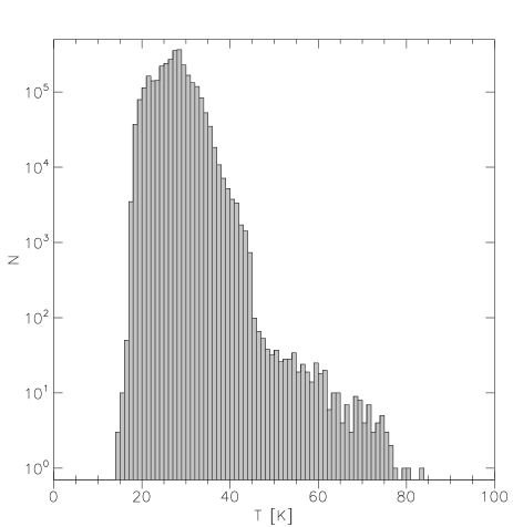
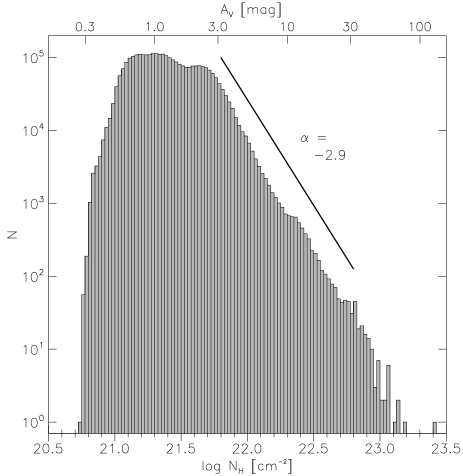
Figure 7: Histogram of 70–160 $\mu$m color temperature values (left) and column density values (right) derived from our maps.

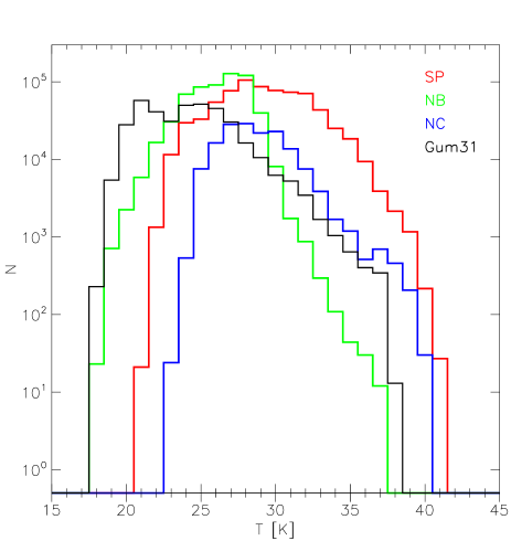
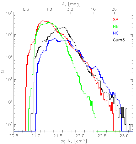
Figure 8: Histogram of 70–160 $\mu$m color temperature (left) column density values (right) for the individual subregions defined in Sect. 3.

6 Column-density- and temperature-distributions and integrated cloud masses in the different parts of the complex

Table 1: Integrated cloud masses for different extinction thresholds.

Region	$M_{\rm tot}$	$M_{\rm tot}$	$M_{\rm tot}$
		$(A_{V}>3)$	$(A_{V}>7)$
	$[M_{\odot}]$	$[M_{\odot}]$	$[M_{\odot}]$
CNC ($R=1\degr$)	655 700	105 100	22 600
SP	209 900	32 300	6940
NC	92 800	44 500	14 300
NB	161 500	4075	185
Gum 31	186 700	46 400	7325

We can now compare the properties of the cloud structure in the different parts of the CNC as defined in Sect. 3. First, we determine the total cloud masses in each region by integrating our column densities over the corresponding area. For the total cloud complex associated to the Carina Nebula we define a circular region with a radius of 1 degree, centered on the position R.A.=10h44m16s, DEC=-59d38m28s (this point is $6.5^{\prime}$ north-east of $\eta$ Car). This region includes nearly all the clouds in our map, but excludes the clouds around Gum 31. Integrating the derived column densities over this circle yields a total cloud mass of $M_{\rm tot}=655\,700\,M_{\odot}$. For the Southern Pillars region we find $209\,900\,M_{\odot}$, and for the Northern Cloud $92\,800\,M_{\odot}$. The integrated mass in the Northern Bubbles region is $161\,500\,M_{\odot}$, and for the Gum 31 region we derive $186\,700\,M_{\odot}$.

While the derived integrated masses should be largely free from background contamination (due to the flux thresholds we applied in our analysis), the gas shows a wide range of densities, from very diffuse and extended low-density filaments to quite massive clouds (like the head of the Northern Cloud). Numerous recent investigations of the relation between cloud structure and the star formation process lead to suggestions of a (column)-density threshold clouds have to exceed in order to allow active star formation. Lada et al. (2010) found that the star formation rate in molecular clouds is linearly proportional to the cloud mass above an extinction threshold of $A_{V}\approx 7$ mag (corresponding to a gas surface density threshold of $\ga 100\,M_{\odot}\,{\rm pc}^{-2}$). The study of Kainulainen et al. (2011) suggested the transition between diffuse clouds and bound clouds (which may be the site of stars formation in the near future) near $A_{V}\approx 3$ mag. We have therefore determined the integrated masses in the above defined regions for all pixels exceeding the column density thresholds of $A_{V}=3$ mag and $A_{V}=7$ mag. These values are listed in Tab. 1.

For the full CNC region, the fraction of mass above $A_{V}=3\,[7]$ mag is 16% [3.4%]. While these fractions are very similar for the Southern Pillars and just slightly higher for the Gum 31 clouds, they are considerably higher (48% [15%]) for the Northern Cloud and considerably lower for the Northern Bubbles (2.5% [0.1%]).

In Fig. 8 we compare the distributions of pixel temperatures and column densities for the four different regions. This shows considerable and remarkable differences between these regions. The clouds in the Southern Pillars show relatively high cloud temperatures. We interprete this as a signature of the strong irradiation that heats these clouds. In combination with the relatively low column densities this suggests that a large fraction of this cloud material is currently in the process of being evaporated due to this heating.

The Northern Bubbles are characterized by systematically lower cloud temperatures. The distribution of column densities is quite similar to that in the Southern Pillars for low extinction values $(A_{V}\la 2$ mag), but drops off very quickly for higher values. This implies that the density contrast in this region is considerably smaller than in the Southern Pillars. This is probably a consequence of the quite different levels and nature of massive star feedback imposed onto these clouds. In the Southern Pillars, the clouds are directly irradiated, what heats their surfaces and can lead to considerable cloud compression in some locations. The Northern Bubbles, on the other hand, are apparently in a situation of less strong irradiation and their structure seems to be dominated by matter flows.

The temperature distribution in the Northern Cloud is quite similar to that in the Southern Pillars. The same is true for the distribution of column densities for values up to $\log\left(N_{\rm H}\right)\leq 22.3$. For higher densities, however, the Northern Cloud shows a prominent excess peak near $\log\left(N_{\rm H}\right)\leq 22.4$, which can be associated to the dense massive center of this cloud.

Finally, the clouds around Gum 31 show relatively low temperatures (with a mode value of 21 K), and intermediate column densities.

It is also interesting to compare the masses derived here from our Herschel maps to those determined from our previous LABOCA map. The total mass of all clouds for which our LABOCA map of the central $1.25\hbox{${}^{\circ}$}\times 1.25\hbox{${}^{\circ}$}$ observed region was sensitive is $60\,000\,M_{\odot}$ (Preibisch et al. 2011a). Considering the same area in our Herschel maps, we find here a total mass of $427\,000\,M_{\odot}$, with $90\,200\,M_{\odot}$ above the $A_{V}\geq 3$ mag threshold. This agrees well with the expectation that LABOCA traces only the mass of the denser clouds.

7 Total cloud mass derived from a simple radiative transfer modeling

If we want to determine the total mass of all the clouds in the CNC, we have to take into account that Herschel is not very sensitive to diffuse warm gas at temperatures $\ga 80$ K. However, due to the very high level of massive star feedback, a substantial fraction of the total gas mass could be at such relatively high temperatures. This gas should then be in atomic rather than molecular form. In order to estimate the total mass of the clouds, we therefore have to also consider the emission at shorter wavelengths, in the mid-infrared range.

We constructed the spectral energy distribution (SED) of the above described $1\degr$ radius region (which includes the entire CNC, but excludes the clouds around Gum 31) in the following way: First, we extracted the total fluxes in this region from our Herschel maps and found values of 844 500 Jy in the $70\,\mu$m band, 847 200 Jy in the $160\,\mu$m band, 374 700 Jy in the $250\,\mu$m band, 156 000 Jy in the $350\,\mu$m band, and 56 000 Jy in the $500\,\mu$m band. For fluxes at shorter wavelengths, we use the MSX and IRAS fluxes in the $8-100\,\mu$m range listed in Table 1 in Smith & Brooks (2007), which were derived for a very similar area. Finally, we also added the FIR and mm-band fluxes determined in the recent study by Salatino et al. (2012), who also considered the same area as Smith & Brooks (2007). The resulting global SED of the CNC is shown in Fig. 9.

In order to estimate the total cloud mass from this SED, we repeated the radiative transfer modeling as described in Preibisch et al. (2011a). We emphasize that this radiative transfer modeling is not intended to be detailed and highly accurate, but just to see whether we can reproduce the general shape of the observed SED with reasonable assumptions about the mass and large-scale density distribution of the surrounding clouds. We do not intend to model the small-scale structure of the individual clouds; instead, we simply assume a central source of radiation surrounded by a spherical envelope of dust and gas. Although this is obviously a strong simplification, it provides the advantage that the temperature distribution of the gas is computed in a more physically meaningful way than adding up a few discrete graybody components.

Since a full description of the radiative transfer modeling was already given in Preibisch et al. (2011a), we summarize here just the main parameters and results:

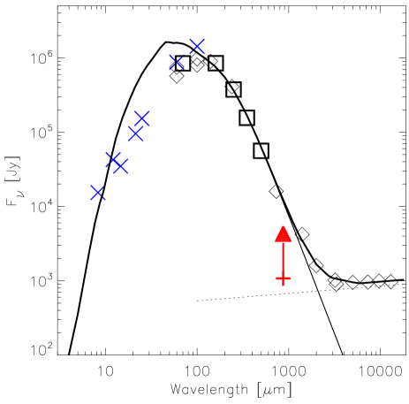
Figure 9: Spectral energy distribution of the Carina Nebula complex. The thick squares show the fluxes derived from our Herschel maps for a $1\degr$ radius area. The crosses show the mid- and far-infrared fluxes determined from the IRAS and MSX maps by Smith & Brooks (2007) for a very similar region. The cross with the upward triangle shows the lower limit to the total $870\,\mu$m flux derived from our LABOCA map that covered the central $1.25\degr\times 1.25\degr$ area. The diamond symbols show the fluxes taken from Salatino et al. (2012). The thick solid line is the sum of the spectrum resulting from the radiative transfer model and a power-law spectrum of the form $F_{\nu}=1100\leavevmode\nobreak\ {\rm Jy}\,\left(\frac{3.4\,{\rm cm}}{\lambda}\right)^{-0.1}$ (following Salatino et al. 2012).

The inner and outer edges of the spatial grid were set at $r=10^{18}$ cm (0.3 pc) and 41 pc. Following the census of massive stars in the CNC by Smith (2006), we assumed a total stellar luminosity of $2.4\times 10^{7}\,L_{\odot}$ and a typical temperature of $T_{\rm eff}=44\,700$ K. The model shown in Fig. 9 assumes that the density increases with distance from the center according to $\rho(r)\propto r^{1.35}$ for radii up to 20.4 pc and then stays constant up to the outer radius at 41 pc; this should approximately match the conditions in the CNC, where most of the cloud material has already been dispersed from the central region and is now located at the periphery of the complex.

The model shown in Fig. 9 contains a total (dust + gas) mass of $889\,140\,M_{\odot}$. The spectrum of this simple model matches the observed FIR fluxes for $\lambda>100\,\mu$m quite well. The fluxes at shorter wavelengths are not so well reproduced, but the model fluxes generally are within a factor of $\sim 2-3$ of the observed values. We note that a good fit of this part on the SED is not expected from our simple model. The apparent discrepancy is probably the consequence of the fact that the true temperature distribution is much more complex than our simple model. Since our model SED predicts systematically too high fluxes in the $15-60\,\mu$m range, the derived mass should be considered to be an upper bound to the total mass.

We also note that the LABOCA $870\,\mu$m flux of 729 Jy is clearly just a lower limit, because the LABOCA map covers just the central $\sim 50\%$ of the analyzed region in our Herschel map. This also explains why the mass derived from this modeling is larger than our previous estimate ($\la 280\,000\,M_{\odot}$) based on the smaller area of the LABOCA map.

It is interesting to compare our result to previous mass estimates of the CNC based on fits of the SED with a few blackbody curves. The SED modeling of Smith & Brooks (2007), who used a combination of three discrete blackbody curves with temperatures of 35 K, 80 K, and 220 K suggested a total (dust + gas) mass of $\approx 962\,000\,M_{\odot}$, slightly higher but still well consistent with our result of $\leq 890\,000\,M_{\odot}$. The SED model of Salatino et al. (2012), which was based on a single temperature component with $T=34.5$ K, yielded a total dust + gas mass of $\approx 950\,000\,M_{\odot}$. Despite the uncertainties (e.g., due to the dust opacity), the results of these different approaches to measure the total mass agree remarkably well.

8 Conclusions and summary

Our Herschel maps show the FIR morphology of the clouds in the CNC at unprecedented sensitivity and angular resolution. They reveal the very complex and filamentary structure of the clouds, which seems to be dominated by the radiation and wind feedback from the numerous massive stars.

The total (gas + dust) mass in the CNC traced by Herschel is $\approx 650\,000\,M_{\odot}$, and our radiative transfer modeling suggests that, including also warmer gas that is not well traced by Herschel, the total mass may be as high as $\leq 890\,000\,M_{\odot}$. Most of this mass resides in clouds with rather low densities. Nevertheless, there are about $105\,000\,M_{\odot}$ in clouds above the extinction threshold of $A_{V}>3$ and about $22\,600\,M_{\odot}$ above $A_{V}>7$. The lower of these two extinction values ($A_{V}>3$) is generally considered to constitute the threshold above which the gas is confined in gravitationally bound entities, making it available for future star formation. The $A_{V}>7$ threshold is though to distinguish the gas that is dense enough to be directly involved in active star formation. We note that Lada et al. (2010) have demonstrated a good correlation between the gas mass above $A_{V}>7$ and the star formation rate, that seems to be valid over a very wide range of cloud masses. This relation predicts a star formation rate of the order $10^{-3}\,M_{\odot}\,{\rm yr}^{-1}$ for the CNC, which is well consistent with the integrated mass and age distribution of the young stars that have formed recently in these clouds (see Preibisch et al. 2011c).

Another important aspect is the ratio between molecular and atomic gas in the complex. Our Herschel maps trace the FIR dust emission and thus our total (gas + dust) mass estimate of $\approx 650\,000-890\,000\,M_{\odot}$ includes both components, i.e. molecular and atomic gas. The amount of the molecular gas can be inferred from molecular line observations. Yonekura et al. (2005) presented a wide-field ¹²CO (J=1–0) survey of the CNC and determined the total gas masses in different sub-regions. Our 1 degree region we used for our CNC mass estimates includes their regions No 1, 2, 3, 7, as well as some parts of their region 4 (see their Table 1 and Fig. 3). Adding up their numbers for the total gas mass based on the ¹²CO signal gives $M_{12\rm CO}\approx 200\,000\,M_{\odot}$. This comparison suggests that about 25% of all the gas in the region is in molecular form, while 75% is in atomic form. We note that the quoted percentages suffer from considerable uncertainties: on the one hand, the CO data may seriously under-estimate the total molecular mass, and on the other hand, uncertainties of the assumed dust opacity and calibration problems may affect the estimate of the total gas mass. Nevertheless, the suggested high mass fraction of atomic gas may be interpreted as the consequence of the high level of massive star feedback that irradiates, heats, and disperses the clouds since several million years. The feedback has apparently transformed much, presumably most, of the original molecular cloud mass into atomic gas.

The Herschel maps provide much more detailed information than reported in this paper. The Herschel fluxes have been used in our recent study of the infrared detected jet-driving protostars in the Carina Nebula (Ohlendorf et al. 2012). In forthcoming publications we will report results about the detailed small-scale structure of the clouds, the numerous point-like FIR sources (most of which are expected to be embedded protostars), as well as the relation between the CNC and the Gum 31 nebula.