Cosmological model with variable equations of state for matter and dark energy

Abstract

We construct a cosmological model which is physically reasonable, mathematically tractable, and extends the study of CDM models to the case where the equations of state (EoS) for matter and dark energy (DE) vary with time. It is based on the assumptions of (i) flatness, (ii) validity of general relativity, (iii) the presence of a DE component that varies between two asymptotic values, (iv) the matter of the universe smoothly evolves from an initial radiation stage - or a barotropic perfect fluid - to a phase where it behaves as cosmological dust at late times. The model approximates the CDM ones for small $z$ but significantly differ from them for large $z$. We focus our attention on how the evolving EoS for matter and DE can modify the CDM paradigm. We discuss a number of physical scenarios. One of them includes, as a particular case, the so-called generalized Chaplygin gas models where DE evolves from non-relativistic dust. Another kind of models shows that the current accelerated expansion is compatible with a DE that behaves like pressureless dust at late times. We also find that a universe with variable DE can go from decelerated to accelerated expansion, and vice versa, several times.

PACS numbers: 98.80.Es, 98.80.-k, 95.36.+x, 98.80.Cq, 04.20.-q

Keywords: Cosmological constant, Cosmology, Einstein equation, general relativity, Dark energy, Cosmic Late-time Acceleration

1 Introduction

One of the most challenging problems in cosmology today is to explain the observed late-time accelerated expansion of the universe [1]-[14]. Since the gravity of both baryonic (ordinary) matter and radiation is attractive, the fact that the universe is presently accelerating, and may continue to do so, forces us to rethink and question some fundamental concepts about the universe.

The first question highlights our limited knowledge of the real nature of the content of the universe. In fact, an accelerated expansion requires the presence of a new form of matter (called dark energy), which could (i) produce gravitational repulsion, i.e., violate the strong energy condition; (ii) account for $70\%$ of the total content of the universe; (iii) remain unclustered on all scales where gravitational clustering of ordinary matter is seen. (For a recent review see Ref. [18]). While we do not yet know exactly the physical mechanism responsible for this exotic behavior, we do have possible candidates for dark energy (DE). They include: a cosmological constant or a time dependent cosmological term [19]-[20]; an evolving scalar field known as quintessence ($Q$-matter) with a potential giving rise to negative pressure at the present epoch [21]-[24]; dissipative fluids [25]; Chaplygin gas [26]-[27]; K-essence [28]-[31], and other more exotic models [32].

The second question is whether general relativity is applicable to describe the universe as a whole. Indeed, this and other puzzles of theoretical and experimental gravity have triggered a huge interest in alternative theories of gravity (See, e.g. [33] and references therein) where the cosmological acceleration is not provided by dark energy, but rather by a modification of the Friedman equation on large scales [34], [35]. These include scalar-tensor theories of gravity [36]-[42], various versions of Kaluza-Klein theories, braneworld, STM and Brans-Dicke theory in $5D$ [43]-[46].

In view of these uncertainties, much of the research work being done in cosmology is based on the construction and study of specific cosmological models. The simplest one that predicts accelerated cosmic expansion and fits observational data reasonably well is the $\Lambda$CDM model [1]-[4] which is based on the assumptions of (i) flatness, (ii) validity of general relativity, (iii) the presence of a cosmological constant $\Lambda$ and (iv) Cold Dark Matter (CDM). The main problem of this model is the huge difference between the observed value of the cosmological constant and the one predicted in quantum field theory. The other one, although not vital for the model, is that the assumption of CDM can not be applied to the entire evolution of the universe.

In this work, we construct an alternative cosmological model where we keep the first two assumptions but relax the other two. Rather than choosing to investigate constraints on specific DE models, here we use a parameterization originally proposed by Hannestad and Mörtsell [47] which can accommodate a number of DE models, including a cosmological constant. On the other hand, we employ a phenomenological approach to describe the matter content of the universe as a mixture of different components, which are not required to expand adiabatically. The mixture smoothly evolves from an initial dense radiation stage - or a barotropic perfect fluid - to a phase where it behaves as cosmological dust at late times.

This framework allows us to compare and contrast different physical settings and tackle a number of questions. Here we focus our attention on the evolution of the universe and its cosmic acceleration and on how the evolving EoS for matter and DE might modify the $\Lambda$CDM paradigm. We explore whether DE could play a significant role in the past evolution of our universe, and - conversely - whether the primordial EoS of matter can affect the details of accelerated expansion at late times. Also, whether dark energy can cross the line between quintessence and phantom regimes (the crossing of the cosmological constant boundary) [48]. Another important question is whether the accelerated expansion, once begun, continues forever: Is it possible for an ever-expanding DE-dominated universe to go through different cycles in which it changes from decelerated to accelerated expansion, and vice versa?

This paper is organized as follows. In section $2$ we give a brief introduction to Einstein’s equations in a homogeneous and isotropic background. In section $3$ for the sake of generality we integrate the field equations without assuming any specific EoS. In this way we obtain general expressions for the Hubble, density and deceleration parameters which in practice provide a simple recipe for the construction of cosmological models. In section $4$ we introduce the EoS that generate our cosmological model and obtain explicit expressions for the relevant cosmological quantities. In section $5$ we study the properties of a universe whose matter content is described by the EoS proposed in section $3$, and the DE has a constant EoS. In section $6$, in the context of CDM, we concentrate our study to the effects of a DE with variable EoS. In section $7$ we present a summary of our work.

2 Field equations

A spatially homogeneous and isotropic universe is described by the FLRW line element, which in polar coordinates $(r,\theta,\varphi)$ is written as

$$ds^{2}=dt^{2}-a^{2}(t)\left[\frac{dr^{2}}{1-kr^{2}}+r^{2}(d\theta^{2}+{\sin}^{2}\theta d\varphi^{2})\right],$$ (1)

where $a(t)$ is the scale factor with cosmic time $t$; $k$ is the curvature signature which can, by a suitable scaling of $r$, be set equal to $-1$, $0$ or $+1$.

The evolution of the scale factor and the stress energy in the universe are governed by the Einstein field equations:

$$R_{\mu\nu}-\frac{1}{2}g_{\mu\nu}R=T_{\mu\nu}.$$ (2)

The assumption of isotropy and homogeneity (1) requires that the stress-energy tensor take on the perfect fluid form: $T_{\nu}^{\mu}=\mbox{diagonal}\left(\rho,-p,-p,-p\right)$, where $\rho$ and $p$ stand for the total energy density and total isotropic pressure of the cosmological “fluid”. This framework leads to two independent equations

$$\frac{3{\dot{a}}^{2}}{a^{2}}+\frac{3k}{a^{2}}=\rho=\sum_{i=1}^{N}\rho^{(i)},$$ (3)

and

$$\frac{2\ddot{a}}{a}+\frac{{\dot{a}}^{2}}{a^{2}}+\frac{k}{a^{2}}=-p=-\sum_{i=1}^{N}p^{(i)},$$ (4)

where an over-dot indicates ordinary derivative with respect to $t$. The total energy density and pressure have been split up into constituents: $\rho^{(i)}$ and $p^{(i)}$ represent the energy density and pressure of the $i$-th component that fills the universe; the sums are over all, say $N$, different species of matter present in the universe (baryonic, non-baryonic, radiation, cosmic neutrinos, dark energy, etc.) at a given epoch.

These equations can be combined to obtain the continuity equation

$$\dot{\rho}+3\left(\rho+p\right)\frac{\dot{a}}{a}=0,$$ (5)

which is equivalent to the covariant conservation equation $T^{\mu\nu}_{\;\;\;;\nu}=0$.

Thus, there are two independent equations and $(2N+1)$ unknown quantities, namely, $a(t)$, $\rho^{(i)}$, $p^{(i)}$, $i=1..N$. To close the system we need to provide $(2N-1)$ additional equations. They could be $N$ equations of state (EoS) relating the pressures and densities. The remaining $\left(N-1\right)$ equations are usually generated by the assumption that each component is expanding adiabatically, i.e., that there is no interaction between the cosmological constituents. What this means is that one imposes the energy conservation equation (5) on each constituent.

The scale factor $a(t)$ can be expressed as a Taylor series around the present time $t_{0}$:

$$\frac{a(t)}{a_{0}}=1+H_{0}\left(t-t_{0}\right)-\frac{1}{2}q_{0}H_{0}^{2}\left(t-t_{0}\right)^{2}+\frac{1}{6}r_{0}H_{0}^{3}\left(t-t_{0}\right)^{3}+...,$$ (6)

where $H=\dot{a}/a$ is the Hubble parameter, which is given directly by (3); $q=-\ddot{a}a/\dot{a}^{2}$ is the deceleration parameter that can be evaluated from (4). If the $i$-th component has an EoS $p^{(i)}=w^{(i)}\rho^{(i)}$ then

$$q=\frac{1}{2}\left[1+3\sum_{i=1}^{N}w^{(i)}\Omega^{(i)}\right]+\frac{k}{2a^{2}H^{2}},$$ (7)

where $\Omega^{(i)}=\rho^{(i)}/3H^{2}$ is the corresponding density parameter. Next, $r=\stackrel{{\scriptstyle\cdots}}{{a}}/aH$ is the statefinder parameter introduced by Sahni et al. [49] and Ulam et al. [50]. Taking time derivative in (4) we obtain

$$r=1-\frac{1}{2H^{3}}\sum_{i=1}^{N}\left[{\dot{w}}^{(i)}\rho^{(i)}+w^{(i)}{\dot{\rho}}^{(i)}\right]+\frac{k}{a^{2}H^{2}}.$$

If, for the sake of generality, the interplay between the constituents is not neglected then each one evolves as

$${\dot{\rho}}^{(i)}+3H\left[1+w^{(i)}\right]\rho^{(i)}=Q^{(i)},\;\;\;\mbox{with}\;\;\;\sum_{i=1}^{N}Q^{(i)}=0,$$

where $Q^{(i)}$ measures the strength of the interaction of the $i$-th constituent with the rest of the components. Using this equation, the parameter $r$ becomes

$$r=1+\frac{3}{2}\sum_{i=1}^{N}\left\{3w^{(i)}\left[1+w^{(i)}\right]-a\,\frac{dw^{(i)}}{da}\right\}\Omega^{(i)}-\frac{1}{2H^{3}}\sum_{i=1}^{N}w^{(i)}Q^{(i)}+\frac{k}{a^{2}H^{2}}.$$ (8)

In a similar way, one can express higher order terms in (6) as functions of $w^{(i)}$, $Q^{(i)}$ and their derivatives.

3 General integration of the field equations

The purpose of this section is to integrate the field equations with the least possible number of assumptions. With this in mind, it is convenient to split up the total energy density and pressure as

$$\rho = \rho^{(DE)}+\rho^{(M)},$$

$$p = p^{(DE)}+p^{(M)},$$ (9)

where $\rho^{(DE)}$ and $p^{(DE)}$ represent the DE contribution and

$$\rho^{(M)}=\sum_{i}\rho^{(i)},\;\;\;p^{(M)}=\sum_{i}p^{(i)},$$ (10)

are hybrids containing the contribution of relativistic particles, photons, the three neutrino species, as well as the contribution of non-relativistic particles (baryons, WIMPS, etc.).

In term of these quantities the field equations (3)-(4) now contain five unknowns. Here, we formulate no assumptions regarding the nature of the expansion of the constituents of the matter mixture $\rho^{(M)}$; they may evolve non-adiabatically. However, to make the problem solvable, we neglect any matter-DE interaction and assume that the DE component is expanding adiabatically. As a result, $\rho^{(DE)}$ and $p^{DE}$, as well as the effective quantities $\rho^{(M)}$ and $p^{M}$, satisfy the continuity equation (5) separately.

To close the system of equations we should provide two EoS. The simplest equation of state between density and pressure is the so called barotropic equation $p/\rho=w$, where $w$ - in relativistic units - is a dimensionless constant. A direct generalization to this equation is to assume that $w$ is not a constant but a function of the epoch. In this work we assume that both, matter and DE satisfy such type of EoS, viz.,

$$p^{(M)} = w(a)\,\rho^{(M)},$$

$$p^{(DE)} = W(a)\,\rho^{(DE)}.$$ (11)

To explain the accelerated expansion one has to accept that the DE component violates the strong energy condition. Thus, in what follows we assume $W(a)<-1/3$.

$\bullet$ With these assumptions the field equations (3)-(4) become

$$\Omega^{(M)}+\Omega^{(DE)}=1+\frac{k}{a^{2}H^{2}},$$ (12)

and

$$q=\frac{1}{2}+\frac{3}{2}\left[W\Omega^{(DE)}+w\Omega^{(M)}\right]+\frac{k}{2a^{2}H^{2}},$$ (13)

where $\Omega^{(M)}=\rho^{(M)}/3H^{2}$ and $\Omega^{(DE)}=\rho^{(DE)}/3H^{2}$. These can, formally, be regarded as two equations for $\Omega^{(M)}$ and $\Omega^{(DE)}$. Solving them we get

$$\Omega^{(M)} = \frac{2q-1-3W}{3\left(w-W\right)}-\frac{k\left(1+3W\right)}{3a^{2}H^{2}\left(w-W\right)},$$

$$\Omega^{(DE)} = -\frac{2q-1-3w}{3\left(w-W\right)}+\frac{k\left(1+3w\right)}{3a^{2}H^{2}\left(w-W\right)}.$$ (14)

We note that the denominator in these expressions is always positive because $W\leq 0$ for DE, as well as for Chaplygin gas models. Thus, the fact that $\Omega^{(M)}\geq 0$ and $\Omega^{(DE)}\geq 0$ imposes an upper and lower limit on $q$, viz.,

$$\frac{1+3W}{2}\left[1+\frac{k}{a^{2}H^{2}}\right]\leq q\leq\frac{1+3w}{2}\left[1+\frac{k}{a^{2}H^{2}}\right].$$ (15)

In the epoch where $0\leq\ \Omega^{(M)}\leq 1/2$ the upper limit reduces to

$$q\leq\frac{1}{2}+\frac{3}{4}\left[w+W\right]+\frac{k}{2a^{2}H^{2}}\left[1+3w^{(\pm)}\right],$$ (16)

where $w^{(+)}=W$ if $k=1$, and $w^{(-)}=w$ if $k=-1$. For the $\Lambda$CDM model the first inequality gives $-1\leq q\leq 1/2$ during the whole evolution and $-1\leq q\leq-1/4$ in the DE dominated era.

$\bullet$ Given the EoS (3), the continuity equations for $\rho^{(M)}$ and $\rho^{(DE)}$ can be formally integrated to obtain the evolution of the energy densities as

$$\rho^{(M)} = \frac{C_{1}}{a^{3}}e^{-3\int{\frac{w(a)}{a}da}},$$

$$\rho^{(DE)} = \frac{C_{2}}{a^{3}}e^{-3\int{\frac{W(a)}{a}da}},$$ (17)

where $C_{1}$ and $C_{2}$ are constants of integration. Let us use $a_{*}$ to denote the epoch at which $\rho^{(M)}(a_{*})=\rho^{(DE)}(a_{*})$, and - for algebraic simplicity - introduce the dimensionless quantity

$$x\equiv\frac{a}{a_{*}}.$$ (18)

Using this notation, without loss of generality, we can write

$$\rho^{(M)} = \frac{C}{x^{3}}e^{-3\int_{1}^{x}{\frac{w(u)}{u}du}},$$

$$\rho^{(DE)} = \frac{C}{x^{3}}e^{-3\int_{1}^{x}{\frac{W(u)}{u}du}},$$ (19)

where $C$ represents the common value shared by the densities at the transition point $x=1$ ($a=a_{*}$). Since $W<0$ and $w\geq 0$, it follows that $\rho^{(M)}>\rho^{(DE)}$ for $x<1$, and vice versa.

In what follows we denote

$$F(x) = e^{-3\int_{1}^{x}{\frac{w(u)}{u}du}},$$

$$G(x) = e^{-3\int_{1}^{x}{\frac{W(u)}{u}du}}.$$ (20)

$\bullet$ The more accepted interpretation of the observational data is that the current universe is very close to a spatially flat geometry ($k=0$), which seems to be a natural consequence from inflation in the early universe. In accordance with this, in the rest of the paper we will consider a flat ($k=0$) universe.

The Friedmann equation (3) with $k=0$ becomes

$$3H^{2}=\frac{C}{x^{3}}\left[F(x)+G(x)\right].$$ (21)

Thus, the density parameters are

$$\Omega^{(M)}=\frac{F(x)}{F(x)+G(x)},\;\;\;\;\Omega^{(DE)}=\frac{G(x)}{F(x)+G(x)}$$ (22)

Since $F(1)=G(1)=1$ it follows that $\Omega^{(M)}=\Omega^{(DE)}=1/2$ at $x=1$, as expected. Now, taking the derivative we find

$$\frac{d\Omega^{(M)}}{dx}=\frac{3\left[W(x)-w(x)\right]}{x}\Omega^{(M)}\Omega^{(DE)}.$$ (23)

This shows that $\Omega^{(M)}$ is a strictly decreasing function of $x$ as long as $\left[W(x)-w(x)\right]<0$, which is always the case for the mixture of DE $(W<0)$ and matter $(w\geq 0)$. It goes from some $1/2<\Omega^{(M)}(0)\leq 1$ to $\Omega^{(M)}(x\rightarrow\infty)\geq 0$. What this means is that there is a one-to-one correspondence between $\Omega^{(M)}$ and $x$. Therefore, if we know its value today then (22) allows us to compute $x_{0}$ by solving the equation (as we mentioned before, the subscript zero denotes the quantities given at the current epoch)

$$F(x_{0})=\left[\frac{\Omega_{0}^{(M)}}{\Omega_{0}^{(DE)}}\right]G(x_{0}).$$ (24)

$\bullet$ The solution to this equation allows us to introduce the cosmological redshift $z$ in term of which $a=a_{0}/(1+z)$. The relationship between $x$, defined in (18), and $z$ is

$$z=\frac{x_{0}}{x}-1.$$ (25)

In particular, the transition from a matter-dominated era to a DE-dominated one occurs at the redshift $z_{*}$ given by

$$z_{*}=x_{0}-1.$$ (26)

Clearly,

$$\left(\frac{a_{0}}{a_{*}}\right)=x_{0}\left\{\begin{array}[]{cc}>1,\;\;z_{*}>0&\mbox{for $\Omega_{0}^{(M)}<1/2$},\\ =1,\;\;z_{*}=0&\mbox{for $\Omega_{0}^{(M)}=1/2$},\\ <1,\;\;z_{*}<0&\mbox{for $\Omega_{0}^{(M)}>1/2$}.\end{array}\right.$$ (27)

Thus, $x_{0}>1$ indicates that the universe became DE dominated in the past; $x_{0}<1$ that DE will dominate in the future, and $x_{0}=1$ that $\Omega_{0}^{(M)}=\Omega_{0}^{(DE)}=1/2$, i.e., that the DE-domination begins right now.

From (24) and (26) we find

$$\frac{dx_{0}}{d\Omega_{0}^{(DE)}}=\frac{dz_{*}}{d\Omega_{0}^{(DE)}}=-\frac{x_{0}}{3\Omega_{0}^{(M)}\Omega_{0}^{(DE)}\left[W(x_{0})-w(x_{0})\right]},$$ (28)

which is always positive. This shows that the closer is $\Omega_{0}^{(DE)}$ to $1^{-}$, the higher the redshift $z_{*}$ - i.e., the further back in time is the transition to the DE-dominated era.

Now we can evaluate the constant $C$. Using (21) and (24) we find

$$C=\frac{3H_{0}^{2}x_{0}^{3}\Omega_{0}^{(M)}}{F(x_{0})}=\frac{3H_{0}^{2}x_{0}^{3}\Omega_{0}^{(DE)}}{G(x_{0})}.$$ (29)

With this quantity at hand, the Hubble parameter (21) can be written as

$$H=H_{0}\left(\frac{x_{0}}{x}\right)^{3/2}\left[\Omega_{0}^{(M)}\frac{F(x)}{F(x_{0})}+\Omega_{0}^{(DE)}\frac{G(x)}{G(x_{0})}\right]^{1/2}.$$ (30)

$\bullet$ The deceleration parameter can be obtained from this expression by using

$$q=-\frac{x}{H}\frac{dH}{dx}-1,$$ (31)

or directly from (13) with $k=0$. Either way we find

$$q(x)=\frac{\left[1+3w(x)\right]F(x)+\left[1+3W(x)\right]G(x)}{2\left[F(x)+G(x)\right]}.$$ (32)

In a similar manner, the deceleration parameter today is obtained immediately from (13) with $k=0$, as

$$q_{0}=\frac{1}{2}\left\{1+3\left[\Omega_{0}^{(M)}w(x_{0})+\Omega_{0}^{(DE)}W(x_{0})\right]\right\},$$ (33)

where $x_{0}$ is the solution to (24) for a given $\Omega_{0}^{(M)}$.

The function $F(x)$ decreases, and $G(x)$ increases, with the increase of $x$. Besides $W<-1/3$. Therefore, at some point $q$ changes its sign from positive to negative. Let us use $\bar{x}$ to denote the root(s) of the equation

$$q(\bar{x})=\left[1+3w(\bar{x})\right]F(\bar{x})+\left[1+3W(\bar{x})\right]G(\bar{x})=0.$$ (34)

It should be noted that it may have several real roots because $q$ is not necessarily a monotonically decreasing function of $x$. In fact, from (32) we get

$$\frac{dq}{dx}=\frac{3\Omega^{(M)}}{2}\frac{dw}{dx}-\frac{9\Omega^{(M)}\Omega^{(DE)}}{2x}\left[w-W\right]^{2}+\frac{3\Omega^{(DE)}}{2}\frac{dW}{dx}$$ (35)

In this expression the first term is non positive, $\left(dw/dx\right)\leq 0$, since the EoS of ordinary matter should become softer - or at most remain constant - during the expansion of the universe. The second one is negative. The third term could, in principle, be positive, zero or negative depending on the specific model. Therefore, an EoS for DE having a large positive slope may lead to several real solutions in (34) and the universe would pass from deceleration to acceleration, and vice versa, several times during its evolution. In general, the only sure thing about the global behavior of $q$ is provided by the inequalities (15) and (16). In summary, if $\left(dW/dx\right)\leq 0$ then $q$ is a strictly decreasing function of $x$ and one can affirm that (34) has only one solution.

Finally, we note that the acceleration of the universe at the end of the matter dominated phase, is given by

$$q_{*}=q(a_{*})=q(x=1)=\frac{1}{2}+\frac{3}{4}\left[w(1)+W(1)\right],$$ (36)

where we have used that $F(1)=G(1)=1$. Clearly, if $q_{*}<0$ then the universe comes into an accelerated expansion, at some $\bar{x}<1$, during the period when matter still dominates over the dark energy component. In contrast, if $q_{*}>0$ then the accelerated expansion begins, at some $\bar{x}>1$, only after the DE component dominates over matter. If $q_{*}=0$ then the onset of accelerated expansion coincides with the end of the matter-dominated era.

4 Cosmological Model with variable EoS for matter and DE

The formulae developed in the preceding sections give the cosmological parameters $\left(H,\Omega,q,r\right)$ explicitly in terms of $w$, $W$, $F$ and $G$. Also (24)-(25) allow to express them as functions of the redshift. What we need now, to construct a cosmological model, is to have the appropriate EoS. In this section we do three things. First, we introduce a variable EoS for the matter mixture (10), and discuss its features. Second, we study a simple parameterization for DE where $W$ varies between two asymptotic values. Third, we present the explicit expressions for the Hubble, density and deceleration parameters.

4.1 Effective EoS for the matter mixture

In the approximation where relativistic matter is modeled by radiation and non-relativistic matter by dust, to describe the evolution of the universe from an early radiation-dominated phase to the recent DE-dominated phase the function $w$ must satisfy the conditions $w\rightarrow 1/3$ for $x\ll 1$, and $w\rightarrow 0$ for $x\gg 1$. Certainly, there are an infinite number of smooth functions that satisfy these conditions.

To motivate our parameterization of $w$ let us go back to (10). The two main components of the cosmic mixture are provided by relativistic and non-relativistic particles. Therefore,

$$w=\frac{\sum_{i}p^{(i)}}{\sum_{i}\rho^{(i)}}\approx\frac{p^{(NR)}+p^{(R)}}{\rho^{(NR)}+\rho^{(R)}},$$

where $\rho^{(R)}$, $p^{(R)}$ and $\rho^{(NR)}$, $p^{(NR)}$ denote the energy density and pressure contributed by relativistic and non-relativistic particles, respectively. In the approximation under consideration $\rho^{(R)}=3p^{(R)}$ and $p^{(NR)}=0$. Thus,

$$w\approx\frac{1}{3\left[f(x)+1\right]},\;\;\;f(x)=\frac{\rho^{(NR)}}{\rho^{(R)}}$$

The relative contributions of the different components depend on time. During adiabatic expansion $\rho^{(NR)}$ decreases as $x^{-3}$, while $\rho^{(R)}$ does it as $x^{-4}$. Thus, $f(x)\sim x$ - at least - if one ignores interactions where an individual kind of particle becomes non-relativistic, gets bound, or annihilates. In this paper we assume $f(x)=Kx^{\alpha}$, where $K$ is a constant of proportionality and $\alpha$ is a positive constant parameter. Thus, we adopt the following very simple approximation

$$w=\frac{1}{3\left(Kx^{\alpha}+1\right)}.$$ (37)

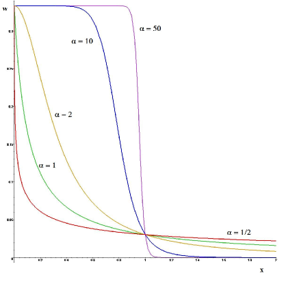
Figure 1: The effective EoS (37) for the matter mixture (10). The Figure shows that for large values of $\alpha$ the transition from radiation to dust is very abrupt, and vice versa. The EoS at $x=1$ is given by $w_{*}=1/3\left(K+1\right)$. For the sake of illustration, the graphic was constructed with $K=10$.

The parameter $\alpha$ determines the rapidity of the transition from radiation to dust as well as the duration of the radiation-dominated epoch. In fact, differentiating with respect to $x$ we obtain

$$\frac{1}{w}\frac{dw}{dx}=-\frac{\alpha K\,x^{(\alpha-1)}}{Kx^{\alpha}+1}.$$ (38)

What this means is that $w$ has a plateau, namely $w\approx 1/3$, in the early universe for any $\alpha>1$. For $\alpha\leq 1$ there is a rapid variation of $w$ at $x\ll 1$ - there is no radiation-dominated plateau - and the transition to dust occurs very slowly. Besides, the larger the choice of $\alpha>1$ the faster the transition to the dust era $w\approx 0$, which goes on with the increase of $x$. See Fig. 1.

The coefficient $K$ determines the EoS at $x=1$, viz.,

$$w_{*}=w(x=1)=\frac{1}{3\left(K+1\right)}.$$

To have $w_{*}\approx 0$ we assume that $K$ is a large, but finite, number.

The mathematical simplicity of (37) allows us to express all the relevant physical quantities in terms of elementary functions. In fact, substituting (37) into (3) we find

$$\rho^{(M)}=\frac{C_{1}\left(Kx^{\alpha}+1\right)^{1/\alpha}}{x^{4}},\;\;\alpha\neq 0,\;\;\;C_{1}=\left(K+1\right)^{-1/\alpha}C.$$ (39)

Consequently,

$$p^{(M)}=\frac{C_{1}\left(Kx^{\alpha}+1\right)^{\left(1-\alpha\right)/\alpha}}{3x^{4}}.$$ (40)

$\bullet$ As expected, for $\alpha=1$ the constituents of the matter mixture recover their individual identities and $\rho^{(M)}$ separates into radiation and dust in adiabatic expansion, viz.,

$$\rho^{(M)}=\frac{KC_{1}}{x^{3}}+\frac{C_{1}}{x^{4}},\;\;\;\;p^{(M)}=\frac{C_{1}}{3x^{4}}.$$ (41)

For any $\alpha\neq 1$, the EoS giving the relation between $p^{(M)}$ and $\rho^{(M)}$ is given in parametric form by (39) and (40). The explicit expression $p^{(M)}=p^{(M)}(\rho^{(M)})$ is quite cumbersome. However, the asymptotic behavior is as follows:

$\bullet$ For $x\ll 1$,

$$\rho^{(M)}\approx\frac{C_{1}}{x^{4}},\;\;\;p^{(M)}\approx\frac{1}{3}\rho^{(M)},$$

$\bullet$ For $x\gg 1$,

$$\rho^{(M)}\approx\frac{C_{1}\,K^{1/\alpha}}{x^{3}},\;\;\;p^{(M)}=\frac{C_{1}\,K^{\left(1-\alpha\right)/\alpha}}{3x^{\left(3+\alpha\right)}},$$

For $\alpha>0$, the matter pressure decreases with the expansion of the Universe faster than the density. Note that $\rho^{(M)}$ decreases as in cosmological dust models. However, formally, exact dust models correspond to the limit $\alpha\rightarrow\infty$. Bellow, in Section $5.1$, we will discuss the properties of the models having $\alpha\gg 1$.

$\bullet$ For $x\approx 1$, near the transition density $\rho^{(M)}_{*}$ the EoS can be written as

$$p^{(M)}\approx\frac{\left(3K+4\right)\left[\rho^{(M)}\right]^{(\alpha+1)}}{3\left(K+1\right)\left\{2\left(K+2\right)\left[\rho^{(M)}\right]^{\alpha}+K\left[\rho^{(M)}_{*}\right]^{\alpha}\right\}}.$$ (42)

This EoS closely mimics the behavior of the one discussed by Israelit and Rosen [51]-[52] where the pressure and density vary continuously through different epochs in FRW universe models.

4.2 A variable equation of state for DE

To describe the evolution of DE we adopt the EoS proposed by Hannestad and Mörtsell [47], which in our notation becomes

$$W=\frac{{\omega}x^{\beta}+\gamma}{x^{\beta}+1},$$ (43)

where $\beta$, ${\omega}$ and $\gamma$ are constants parameters. If $\omega=\gamma$ then $W=\omega$. In any other case ${\omega}$ and $\gamma$ describe the asymptotic behavior of $W$. Namely, for $\beta>0$

$$W\rightarrow\left\{\begin{array}[]{cc}{\omega}&\mbox{for $x\gg 1$},\\ \gamma&\mbox{for $x\ll 1$}.\end{array}\right.$$ (44)

For $\beta<0$, the constants ${\omega}$ and $\gamma$ interchange their role, i.e., $W\rightarrow\gamma$ for $x\gg 1$ and $W\rightarrow{\omega}$ for $x\ll 1$. In what follows without loss of generality we assume $\beta>0$.

Besides,

$$\frac{dW}{dx}=\frac{\beta x^{\beta-1}\left(\omega-\gamma\right)}{\left(x^{\beta}+1\right)^{2}}$$

shows that for $\beta>1$, $W$ undergoes a rapid transition from an early epoch where $W\approx\gamma$ to a large epoch where $W\approx{\omega}$. In addition, $W$ is an increasing function of $x$ if ${\omega}>\gamma$, and vice versa.

Next, to account for the repulsive nature of DE we should demand the violation of the strong energy condition of classical cosmology. It is easy to verify that $\rho^{(DE)}+3p^{(DE)}=\rho^{(DE)}(1+3W)<0$ in the whole range of $x$ provided

$${\omega}<-\frac{1}{3},\;\;\;\gamma<-\frac{1}{3}.$$ (45)

Lower limits on these quantities, namely ${\omega}>-1$ and $\gamma>-1$ are obtained if one assumes that DE satisfies the dominant energy condition $\rho^{(DE)}\geq|p^{DE}|$.

Substituting (43) into (3), we obtain

$$\rho^{(DE)}=\frac{C_{2}\left(x^{\beta}+1\right)^{-3({\omega}-\gamma)/\beta}}{x^{3(1+\gamma)}},\;\;\beta\neq 0,\;\;\;C_{2}=2^{3\left(\omega-\gamma\right)/\beta}\,C.$$ (46)

Thus,

$$p^{(DE)}=\frac{C_{2}\left({\omega}x^{\beta}+\gamma\right)}{x^{3\left(1+\gamma\right)}\left(x^{\beta}+1\right)^{[3\left({\omega}-\gamma\right)+\beta]/\beta}}.$$ (47)

We immediately notice that for $\beta=3\left(\gamma-\omega\right)$ the above equations reduce to

$$\rho^{(DE)} = C_{2}\left[\frac{1}{x^{3\left(1+\omega\right)}}+\frac{1}{x^{3\left(1+\gamma\right)}}\right],$$

$$p^{(DE)} = C_{2}\left[\frac{\omega}{x^{3\left(1+\omega\right)}}+\frac{\gamma}{x^{3\left(1+\gamma\right)}}\right].$$ (48)

What this means is that for $\beta=3\left(\gamma-\omega\right)$ the DE can be interpreted as the superposition of two fluids with EoS

$$p_{1}=\omega\rho_{1},\;\;\;\;p_{2}=\gamma\rho_{2},$$ (49)

each of which satisfies the continuity equation.

The asymptotic behavior of (46)-(47) is as follows:

$\bullet$ For $x\ll 1$, there are two different physical situations. If $\gamma\neq 0$ we get

$$\rho^{(DE)}\approx\frac{C_{2}}{x^{3(1+\gamma)}},\;\;\;p^{(DE)}\approx\gamma\rho^{(DE)}.$$

In this limit $\rho^{(DE)}/\rho^{(M)}\approx x^{1-3\gamma}$. Therefore $\rho^{(DE)}\ll\rho^{(M)}$ for $x\ll 1$ as long as $\gamma<1/3$.

If $\gamma=0$ we find

$$\rho^{(DE)}\approx\frac{C_{2}}{x^{3}},\;\;\;p^{(DE)}\approx\omega C_{2}x^{\left(\beta-3\right)}.$$

Thus, for $\beta>3$ the DE component - in this limit - behaves exactly as in cosmological dust models.

$\bullet$ For $x\gg 1$ we obtain

$$\rho^{(DE)}\approx\frac{C_{2}}{x^{3\left(1+{\omega}\right)}},\;\;\;p^{(DE)}={\omega}\rho^{(DE)}.$$

Since ${\omega}<0$, it follows that $\rho^{(DE)}\gg\rho^{(M)}$ and $|p^{(DE)}|\gg p^{(M)}$ for $x\gg 1$. Also, in this limit when ${\omega}=-1$ the DE component behaves as a cosmological constant $p^{(DE)}=-\rho^{(DE)}=C_{2}$.

$\bullet$ For $x\approx 1$, the transition from $W\approx\gamma$ to $W\approx{\omega}$ can be approximated by an EoS similar to (42).

Generalized Chaplygin gas:

The above analysis indicates that when ${\omega}=-1$, $\beta>3$ and $\gamma=0$ the DE component evolves from non-relativistic matter (dust) to a cosmological constant, similar to the so-called Chaplygin gas. In fact, it is not difficult to see that for this choice of parameters (46)-(47) yield

$$p^{(DE)}\left[\rho^{(DE)}\right]^{\sigma}=-C_{2}^{\left(1+\sigma\right)},$$ (50)

where $\sigma=(\beta-3)/3$ and

$$\rho^{(DE)}=C_{2}\left[1+\frac{1}{x^{3\left(1+\sigma\right)}}\right]^{1/\left(1+\sigma\right)}.$$ (51)

Thus, the EoS

$$W=-\frac{x^{\beta}}{x^{\beta}+1},$$ (52)

with $3<\beta<6$ describes a generalized Chapligyn gas.

4.3 The Hubble, density and deceleration parameters

We now proceed to apply our general formulae to the EoS (37) and (43). For practical reasons, it is useful to write (37) as

$$w=\frac{n}{\left(Kx^{\alpha}+1\right)},$$ (53)

with n = 1/3. This will allow us to follow in detail, step by step, the possible effects of the primordial radiation on the observed accelerated expansion today. Besides, it allows us to extend our results to include other types of matter, e.g., stiff (incompressible) matter ($n=1$). Also for $n=0$ we should recover the usual CDM picture.

Thus, for the sake of generality in our discussion we let

$$0\leq n\leq 1,$$ (54)

in accordance with the strong and dominant energy conditions.

From (3) we get

$$F(x)=\left(K+1\right)^{-3n/\alpha}\left[K+\frac{1}{x^{\alpha}}\right]^{3n/\alpha},\;\;\;G(x)=\frac{2^{3\left(\omega-\gamma\right)/\beta}}{x^{3\omega}}\left[1+\frac{1}{x^{\beta}}\right]^{-3\left(\omega-\gamma\right)/\beta}.$$ (55)

$\bullet$ The Hubble parameter is obtained by substituting these into (30), namely,

$$H(x)=H_{0}\left[\Omega_{0}^{(M)}\left(\frac{x_{0}}{x}\right)^{3}\,f(x)+\Omega_{0}^{(DE)}\left(\frac{x_{0}}{x}\right)^{3\left(\omega+1\right)}g(x)\,\right]^{1/2},$$ (56)

where we have introduced the functions $f(x)$ and $g(x)$ defined by

$$f(x)=\left[\frac{K+\frac{1}{x^{\alpha}}}{K+\frac{1}{x^{\alpha}_{0}}}\right]^{3n/\alpha},\;\;\;\;g(x)=\left[\frac{1+\frac{1}{x_{0}^{\beta}}}{1+\frac{1}{x^{\beta}}}\right]^{3\left(\omega-\gamma\right)/\beta},$$ (57)

and $x_{0}$ is the solution to (24), which in the case under consideration becomes

$$x_{0}^{3{\omega}}\left(K+\frac{1}{x_{0}^{\alpha}}\right)^{3n/\alpha}\left(1+\frac{1}{x_{0}^{\beta}}\right)^{3({\omega}-\gamma)/\beta}=2^{3({\omega}-\gamma)/\beta}\left(K+1\right)^{3n/\alpha}\left[\frac{\Omega_{0}^{(M)}}{\Omega_{0}^{(DE)}}\right].$$ (58)

The energy densities, from (3), (3), (55), (57), can be written as

$$\rho^{(M)} = \rho^{(M)}_{0}\left(\frac{x_{0}}{x}\right)^{3}f(x),$$

$$\rho^{(DE)} = \rho^{(DE)}_{0}\left(\frac{x_{0}}{x}\right)^{3\left(1+\omega\right)}g(x).$$ (59)

For $n=0$ and $\gamma=\omega$, these expressions reduce to the usual ones in the CDM model, as expected.

$\bullet$ The deceleration parameter is easily obtained by a direct substitution of (43), (53) and (55) into (32). We get

$$q(x)=\frac{x^{3\omega}\left(K+\frac{1}{x^{\alpha}}\right)^{3n/\alpha}\left[\frac{Kx^{\alpha}+1+3n}{Kx^{\alpha}+1}\right]+2^{3\left(\omega-\gamma\right)/\beta}\left(K+1\right)^{3n/\alpha}\left(1+\frac{1}{x^{\beta}}\right)^{-3\left(\omega-\gamma\right)/\beta}\left[\frac{\left(3\omega+1\right)x^{\beta}+\left(3\gamma+1\right)}{x^{\beta}+1}\right]}{2\left[x^{3\omega}\left(K+\frac{1}{x^{\alpha}}\right)^{3n/\alpha}+2^{3\left(\omega-\gamma\right)/\beta}\left(K+1\right)^{3n/\alpha}\left(1+\frac{1}{x^{\beta}}\right)^{-3\left(\omega-\gamma\right)/\beta}\right]}.$$ (60)

We observe that $q(x=0)=\left(1+3n\right)/2$ and $q(x\rightarrow\infty)=\left(1+3{\omega}\right)/2$. Since $\omega<-1/3$, there is at least one value of $x$, say $x=\bar{x}$, for which $q$ vanishes. In accordance with our discussion in (35), $q$ is not necessarily a decreasing function of $x$ if $dW/dx>0$ in which case $q(\bar{x})=0$ may have more than one real root. In Figure 2 we illustrate the situation where $q(x)=0$ has three different roots for different EoS: dust ($n=0$), primordial radiation ($n=1/3$) and stiff matter ($n=1$).

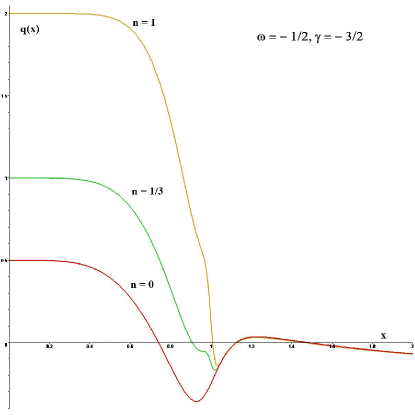
Figure 2: The figure illustrates the situation where the deceleration parameter changes sign several times during the expansion of the universe. We have selected $\omega=-1/2$, $\gamma=-3/2$ and $\beta=20$ to generate a large $dW/dx>0$. Also, we have chosen $\alpha=100$ to assure that the models with primordial radiation ($n=1/3$) and stiff matter $(n=1)$ are indistinguishable from the dust model at late times. Also, for this choice the number of zeroes of $q(x)$ as well as their locations are essentially independent of the specific value of $K$. The graphic was constructed with $K=1$.

In general, only the upper and lower bounds on $q$ are well-defined and are given by (15). In the case under consideration these are

$$\frac{1+3\xi}{2}\leq q\leq 1,\;\;\;\xi=\mbox{min}\left\{\gamma,{\omega}\right\}.$$ (61)

Besides, in agreement with (36) we find that at the transition point $x=1$ ($a=a_{*}$)

$$q_{*}\equiv q(x=1)=\frac{1}{2}+\frac{3\left(\omega+\gamma\right)}{8}+\frac{3n}{4\left(K+1\right)},$$ (62)

regardless of the specific choice of $\alpha$ and $\beta$.

$\bullet$ The magnitude of the deceleration parameter today, $q_{0}$, is readily given by (33), viz.,

$$q_{0}=\frac{1}{2}\left[1+\frac{3n\Omega_{0}^{(M)}}{Kx_{0}^{\alpha}+1}+\frac{3\Omega_{0}^{(DE)}\left({\omega}x_{0}^{\beta}+\gamma\right)}{x_{0}^{\beta}+1}\right].$$ (63)

The same expression can be obtained from (60), after using (58) and some algebraic manipulations.

4.3.1 Cosmological parameters in terms of the redshift

For practical/observational reasons it is convenient to express the cosmological parameters as functions of the redshift $z$ introduced in (25).

The Hubble parameter (56) becomes

$$H^{2}=H_{0}^{2}\left[\Omega_{0}^{(M)}\left(1+z\right)^{3}f(z)+\Omega_{0}^{(DE)}\left(1+z\right)^{3(\omega+1)}g(z)\right],$$ (64)

with

$$f(z) = \left[\frac{Kx_{0}^{\alpha}+\left(1+z\right)^{\alpha}}{Kx_{0}^{\alpha}+1}\right]^{3n/\alpha},$$

$$g(z) = \left[\frac{x_{0}^{\beta}+\left(1+z\right)^{\beta}}{x_{0}^{\beta}+1}\right]^{-3\left({\omega}-\gamma\right)/\beta}.$$ (65)

The energy densities can be written as

$$\rho^{(M)} = 3\left(1+z\right)^{3}\Omega_{0}^{(M)}H_{0}^{2}f(z),$$

$$\rho^{(DE)} = 3\left(1+z\right)^{3\left(1+{\omega}\right)}\Omega_{0}^{(DE)}H_{0}^{2}g(z).$$ (66)

Finally, the deceleration parameter as a function of $z$ is given by

$$q(z)=\frac{H_{0}^{2}}{2H^{2}}\left\{\Omega_{0}^{(M)}\left(1+z\right)^{3}f(z)\frac{\left[Kx_{0}^{\alpha}+\left(3n+1\right)\left(1+z\right)^{\alpha}\right]}{\left[Kx_{0}^{\alpha}+\left(1+z\right)^{\alpha}\right]}+\Omega_{0}^{(DE)}\left(1+z\right)^{3\left(1+{\omega}\right)}g(z)\frac{\left[x_{0}^{\beta}\left(1+3{\omega}\right)+\left(1+z\right)^{\beta}\left(1+3\gamma\right)\right]}{\left[x_{0}^{\beta}+\left(1+z\right)^{\beta}\right]}\right\}.$$ (67)

These equations show that at low redshift $f(z)\approx 1$ and $g(z)\approx 1$ and we recover the usual CDM model, i.e., the dynamics of the EoS for DE and matter only becomes important at hight redshift.

5 Universe of matter with variable EoS and DE with $W=$ constant

We now start the study of the properties of our cosmological model. In this section we concentrate our attention on the question of how a dynamical EoS for matter can alter the details of the accelerated expansion as given by the CDM ($w=0$) models. With this in mind, here we confine the discussion to the case where the DE component has a constant EoS (a variable $W$ will be discussed in the next section).

Thus, in this section

$$W=\omega=\mbox{constant}.$$ (68)

For $\omega=-1$ we have a standard cosmological constant. Setting $\gamma=\omega$, from (58), (60) and (63) we get

$$x_{0}^{3\omega}\left(K+\frac{1}{x^{\alpha}_{0}}\right)^{3n/\alpha}=\left(K+1\right)^{3n/\alpha}\frac{\Omega_{0}^{(M)}}{\Omega_{0}^{(DE)}},$$ (69)

$$q(\bar{x})=\bar{x}^{3\omega}\left[K+\frac{1}{\bar{x}^{\alpha}}\right]^{3n/\alpha}\left[\frac{K\bar{x}^{\alpha}+1+3n}{K\bar{x}^{\alpha}+1}\right]+\left(K+1\right)^{3n/\alpha}\left(1+3\omega\right)=0,$$ (70)

and

$$q_{0}=\frac{1}{2}\left[1+3\omega\Omega_{0}^{(DE)}\right]+\frac{3n\Omega_{0}^{(M)}}{2\left(Kx_{0}^{\alpha}+1\right)},$$ (71)

respectively. Thus, to obtain a numerical value for $q_{0}$ as well as the observational quantities $z_{*}=x_{0}-1$ and $\bar{z}=x_{0}/\bar{x}-1$, we need to solve (69) and (70).

CDM:

For $n=0$, they have a close algebraic solution which is the CDM model, viz.,

$$x_{0}^{(CDM)} = \left[\frac{\Omega_{0}^{(M)}}{\Omega_{0}^{(DE)}}\right]^{1/3\omega},$$

$${\bar{x}}^{(CDM)} = \left[-\left(1+3\omega\right)\right]^{1/3\omega},$$

$$q_{0}^{(CDM)} = \frac{1}{2}\left[1+3\omega\Omega_{0}^{(DE)}\right].$$ (72)

Variable EoS:

For $n\neq 0$, from (69)-(70) we find expressions for $x_{0}$ and $\bar{x}$ which are very similar to those given by (5), namely

$$x_{0} = \left(\frac{w_{0}}{w_{*}}\right)^{n/\alpha\left(\omega-n\right)}\left[\frac{\Omega_{0}^{(M)}}{\Omega_{0}^{(DE)}}\right]^{1/3\left(\omega-n\right)},$$

$$\bar{x} = \left(\frac{\bar{w}}{w_{*}}\right)^{n/\alpha\left(\omega-n\right)}\left[-\frac{1+3\omega}{1+3\bar{w}}\right]^{1/3\left(\omega-n\right)},$$ (73)

where $w_{0}$, $w_{*}$ and $\bar{w}$ represent the EoS (53) evaluated at $x_{0}$, $x=1$ and $x=\bar{x}$, respectively. They reduce to their CDM counterpart for $n=0$, as expected. Although the shape of these expressions is intriguing, to find $x_{0}$ and $\bar{x}$ we need to provide a set of values $(\Omega_{0}^{(M)},\,\omega,\,n,\,K,\,\alpha)$ and then solve numerically.

However, a direct inspection of (69)-(70) suggests that we examine the following cases: (i) $\alpha=3n$; (ii) $0<\alpha\ll 3n$ and (iii) $\alpha\gg 3n$.

$\bullet$ When $\alpha=3n$, the matter in the universe is a superposition of two non-interacting fluids; one of them is dust, and the other one is a fluid with an EoS $p=n\rho$. Specifically,

$$\rho^{(M)}=\frac{KC_{1}}{x^{3}}+\frac{C_{1}}{x^{3\left(n+1\right)}},\;\;\;\;p^{(M)}=\frac{nC_{1}}{x^{3\left(n+1\right)}}.$$ (74)

$\bullet$ When $0<\alpha\ll 3n$ we have

$$\rho^{(M)}=\frac{C_{1}}{x^{3\left(1+\tilde{n}\right)}},\;\;\;\;\tilde{n}=\frac{n}{K+1},$$

$$x_{0}=\left[\frac{\Omega_{0}^{(M)}}{\Omega_{0}^{(DE)}}\right]^{1/3\left(\omega-\tilde{n}\right)},$$ (75)

$$\bar{x}=\left[\frac{-\left(1+3\omega\right)}{1+3\tilde{n}}\right]^{1/3\left(\omega-\tilde{n}\right)}.$$ (76)

Since $K$ is a large number ($K\sim\rho^{(NR)}/\rho^{(R)}\sim 3\times 10^{4}$ today), the above solution is practically indistinguishable from the CDM model (5).

$\bullet$ When $\alpha\gg 3n$, we find that the physics is independent of the particular choice of $K$ and $\alpha$. In the next subsection we discuss the details.

5.1 Asymptotic model: $\alpha\gg 3n$

A simple numerical analysis of (69)-(70), with $(\Omega_{0}^{(M)},\,\omega,\,n,\,K)$ fixed, shows that $x_{0}$ and $\bar{x}$ tend to specific finite limits when $\alpha\rightarrow\infty$. A further analysis demonstrates that these limits are insensitive to the specific choice of $K$.

Therefore, in this limit only the parameters $\omega$, $n$ and $\Omega_{0}^{(M)}$ have physical relevance. It corresponds to the case where the transition to dust occurs abruptly near $x=1$ (See Figures 1, 3, 4 ).

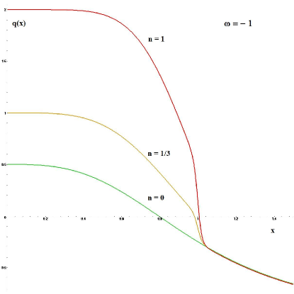
Figure 3: The deceleration parameter $q$ versus $x$ for models with cosmological constant. The figure compares the evolution of $q$ in the $\Lambda$CDM model ($n=0$) to the one in models with $n=1/3$ and $n=1$ calculated for $\alpha=100$ and $K=1$.

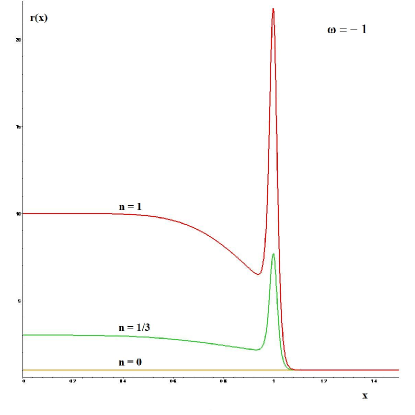
Figure 4: The statefinder parameter $r$, given by (8), versus $x$ for models with cosmological constant. In the $\Lambda$CDM models $r=1$. The sharp peak of $r$ is evidence of the rapid change experienced by the deceleration parameter. Once again we have taken $\alpha=100$ to ensure that the models behave like dust at late times. Moreover $K=1$.

As shown in (27), the character of the solutions to (69) strongly depends on whether the universe is dominated by matter or DE. Accordingly, for $\alpha\gg 1$ we find

$$x_{0}=\left\{\begin{array}[]{cc}x_{0}^{(CDM)}&\mbox{for $\Omega_{0}^{(M)}<1/2$},\\ \left[\frac{\Omega_{0}^{(M)}}{\Omega_{0}^{(DE)}}\right]^{1/3\left(\omega-n\right)}&\mbox{for $\Omega_{0}^{(M)}>1/2$}.\end{array}\right.$$ (77)

For $\Omega_{0}^{(M)}=1/2$, $x_{0}=1$ regardless of the choice of parameters. To simplify the discussion in Table $1$ we calculate $x_{0}$ for various $\Omega_{0}^{(0)}<1/2$ and $\omega$.

Table 1. $x_{0}$ for various $\Omega_{0}^{(M)}$, $\omega$, any $n$ and $\alpha\gg 1$
$\Omega_{0}^{(M)}$	$\omega=-0.4$	$\omega=-0.5$	$\omega=-2/3$	$\omega=-1$	$\omega=-1.3$	$\omega=-1.5$	$\omega=-10$
$0.1$	$6.240$	$4.327$	$3.000$	$2.080$	$1.756$	$1.629$	$1.076$
$0.2$	$3.175$	$2.520$	$2.000$	$1.587$	$1.427$	$1.361$	$1.047$
$0.3$	$2.026$	$1.759$	$1.527$	$1.326$	$1.243$	$1.207$	$1.028$
$0.4$	$1.402$	$1.310$	$1.225$	$1.148$	$1.110$	$1.094$	$1.014$

$\bullet$ By virtue of (35), the EoS (68) guarantees that $q(x)$ is a strictly decreasing function of $x$. Consequently, (70) has only one real root for each set $(\omega,\,n,\,K,\alpha)$. They heavily depend on whether the deceleration-acceleration transition occurs before or after the end of the matter-dominated era. From (36) we find

$$q_{*}=\frac{1}{4}\left(2+3\omega+\frac{3n}{K+1}\right).$$ (78)

What this means is that $\bar{x}\geq 1$ for $\omega\geq-\left[2/3+n/(K+1)\right]$, and vice versa.

Thus, for $\alpha\gg 1$ we obtain the following solutions:

(i) $\omega>-2/3$:

$$\bar{x}=\left[-\left(1+3\omega\right)\right]^{1/3\omega},$$

where the condition $\omega>-2/3$ ensures that $\bar{x}>1$.

(ii) $-\left[2/3+n/(K+1)\right]<\omega\leq-2/3$:

$$\bar{x}=1^{+}.$$

(iii) $\omega=-\left[2/3+n/(K+1)\right]$:

$$\bar{x}=1,$$

for any choice of parameters.

(iv) $-\left(2+3n\right)/3\leq\omega<-\left[2/3+n/(K+1)\right]$:

$$\bar{x}=1^{-}.$$

(v) $\omega<-\left(2+3n\right)/3$:

$$\bar{x}=\left[-\frac{\left(1+3\omega\right)}{\left(1+3n\right)}\right]^{1/3\left(\omega-n\right)},$$

where the condition $\omega<-\left(2+3n\right)/3$ ensures that $\bar{x}<1$.

For $n=0$ we recover the expressions for CDM. In Table $2$ we present the approximate values of $\bar{x}$ for different choices of $\omega$, $n$ and $\alpha\gg 1$. We remark that those for $\omega\geq-2/3$ are independent of $n$ and coincide with the CDM values.

Table 2. $\bar{x}$ for various $\omega$, $n$ and $\alpha\gg 1$
$\omega$	$n=0$	$n=0.1$	$n=0.2$	$n=1/3$	$n=2/3$	$n=1$
$-0.4$	$3.824$	$3.824$	$3.824$	$3.824$	$3.824$	$3.824$
$-0.5$	$1.587$	$1.587$	$1.587$	$1.587$	$1.587$	$1.587$
$-2/3$	$1$	$1$	$1$	$1$	$1$	$1$
$-5/6$	$0.850$	$0.950$	$1$	$1$	$1$	$1$
$-1$	$0.794$	$0.878$	$0.940$	$1$	$1$	$1$
$-1.3$	$0.761$	$0.826$	$0.876$	$0.927$	$1$	$1$
$-1.5$	$0.757$	$0.813$	$0.858$	$0.903$	$0.976$	$1$
$-10$	$0.894$	$0.903$	$0.910$	$0.917$	$0.932$	$0.942$

If $\omega<-2/3$, then our model predicts some changes to the CDM paradigm. First we note that in CDM models (first column in Table $2$) $\bar{x}$ varies with $\omega$. But, this is not necessarily so when $n\neq 0$. Solutions (ii)-(iv) show that $\bar{x}\approx 1$, for every $n$, in the whole range $-\left(2+3n\right)/3\leq\omega\leq-2/3$.

However, the redshift associated with $\bar{x}$ does depend on $\omega$ through $x_{0}$. For example, if we take $n=1/3$ and $\Omega_{0}^{(M)}=0.3$ then Table $1$ gives $x_{0}=\left(1.527,\;1.326\right)$ for $\omega=-2/3$ and $\omega=-1$, respectively. Correspondingly, we get $\bar{z}=\left(0.527,\;0.326\right)$, although $\bar{x}=1$ in both cases.

When $\omega<-\left(2+3n\right)/3$, for $\Omega_{0}^{(M)}<1/2$ the redshift for the deceleration-acceleration transition is given by

$$\bar{z}=\left[\frac{\Omega_{0}^{(M)}}{\Omega_{0}^{(DE)}}\right]^{1/3\omega}\left[-\frac{\left(1+3\omega\right)}{\left(1+3n\right)}\right]^{1/3\left(n-\omega\right)}-1.$$ (79)

For the case where DE is a cosmological constant $(\omega=-1)$ and $\Omega_{0}^{(M)}=0.3$ we get

$$\bar{z}=\left(0.671,\;0.511,\;0.411,\;0.326\right),\;\;\;\mbox{for}\;\;\;n=\left(0,\;0.1,\;0.2,\;1/3\right).$$

We note that the redshift at $q=0$ predicted by the CDM models is a little more than twice the one obtained for $n=1/3$. As a second example we consider phantom DE with $\omega=-1.5$ and, once again, take $\Omega_{0}^{M}=0.3$. We find

$$\bar{z}=\left(0.595,\;0.484,\;0.407,\;0.337,\;0.237,\;0.207\right),\;\;\;\mbox{for}\;\;\;n=\left(0,\;0.1,\;0.2,\;1/3,\;2/3,\;1\right).$$

Thus, for non-phantom ($\omega\geq-1$) and phantom matter $(\omega<-1)$, we can conclude that the stiffer the primordial EoS, the later - i.e. closer to our era - the transition to accelerated expansion.

To finish the discussion, we would like to point out that the asymptotic model discussed here and the CDM model - given by (5) - do not challenge each other. Instead, they are complementary. Indeed, they represent two different limits: in the CDM model dust is assumed during the whole evolution, while here there is a sharp transition from a primordial $n\neq 0$ stage, to cosmological dust. These two asymptotic models should serve to restrict or restrain more realistic ones.

5.2 Features of the model that are independent of $\alpha$ and $K$

In any physical model is important to identify the features that are independent of the particular choice of the parameters of the theory. Therefore, we now look for relationships between the observational parameters that are independent of the particular choice of $\alpha$ and $K$. With this in mind we recast (69) into the form

$$X^{3\omega}\left[1+\frac{1}{X}\right]^{3n}=K^{3\omega}\left[1+\frac{1}{K}\right]^{3n}\left[\frac{\Omega_{0}^{(M)}}{\Omega_{0}^{(DE)}}\right]^{\alpha},$$

where $X=Kx^{\alpha}$. Since, $\alpha>0$, $n\geq 0$ and $\omega<0$, from this equation it follows that $X>K$ for $\Omega_{0}^{(M)}<\Omega_{0}^{(DE)}$; $X<K$ for $\Omega_{0}^{(M)}>\Omega_{0}^{(DE)}$, and $X=K$ for $\Omega_{0}^{(M)}=\Omega_{0}^{(DE)}$. This is consistent with the fact that $x_{0}>1$ ($x_{0}\leq 1$) $\Longleftrightarrow$ $\Omega_{0}^{M}<1/2$ ($\Omega_{0}^{M}\geq 1/2$) discussed in (27).

Now, from (71) we obtain $(n\neq 0)$

$$Kx_{0}^{\alpha}=\frac{3\left(\omega-n\right)\Omega_{0}^{(M)}+2q_{0}-1-3\omega}{3\omega\Omega_{0}^{(DE)}-2q_{0}+1}.$$ (80)

Using this expression we find:

Models with $\Omega_{0}^{(M)}<1/2$:

Setting $Kx_{0}>K$, from (80) we get

$$\frac{1}{2}\left[1+3\omega\Omega_{0}^{(DE)}\right]<q_{0}<\frac{1}{2}\left[1+3\omega\Omega_{0}^{(DE)}\right]+\frac{3}{4}n\Omega_{0}^{(M)}.$$ (81)

As in the CDM models, the current accelerated expansion requires

$$\omega<-\frac{1}{3\Omega_{0}^{(DE)}}.$$ (82)

Equivalently, in terms of $\omega$ the above inequality can be written as

$$\left[\frac{2q_{0}-1}{3\Omega_{0}^{(DE)}}\right]-\frac{n\Omega_{0}^{(M)}}{2\Omega_{0}^{(DE)}}<\omega<\left[\frac{2q_{0}-1}{3\Omega_{0}^{(DE)}}\right]$$ (83)

$\bullet$ For any given $\Omega_{0}^{(M)}<1/2$, this expression yields a lower and/or an upper bound on $q_{0}$ for various values of $\omega$, viz.,

$$q_{0} > -1+\frac{3\Omega_{0}^{(M)}}{2},\;\;\;\mbox{for}\;\;\;\omega>-1,$$

$$q_{0} < -1+\frac{3\left(n+2\right)\Omega_{0}^{(M)}}{4},\;\;\;\mbox{for}\;\;\;\omega<-1,$$

$$-1+\frac{3\Omega_{0}^{(M)}}{2}<q_{0} < -1+\frac{3\left(n+2\right)\Omega_{0}^{(M)}}{4},\;\;\;\mbox{for}\;\;\;\omega=-1.$$ (84)

As an illustration, let us take $\Omega_{0}^{(M)}=0.3$. Then, accelerated expansion requires $\omega<-0.476$; if $\omega>-1$ then the deceleration parameter has a lower bound $q_{0}^{(min)}=-0.550$, regardless of $n$; if $\omega<-1$ it has an upper bound that depends on $n$, namely, $q_{0}^{(max)}=(-0.325,\;-0.447,\;-0.550)$ for $n=(1,\;1/3,\;0)$, respectively; if $\omega=-1$ then $q_{0}$ is bounded from above and from bellow, viz., $-0.550<q_{0}<(-0.325,\;-0.447,\;-0.550)$ for $n=(1,\;1/3,\;0)$, respectively.

Models with $\Omega_{0}^{(M)}=1/2$:

In these models the condition $x_{0}=1$ yields

$$q_{0}=\frac{1}{2}\left[1+\frac{3}{4}\left(n+2\omega\right)\right].$$ (85)

Accelerated expansion at the current epoch requires

$$\omega<-\frac{4+3n}{6}.$$ (86)

Models with $\Omega_{0}^{(M)}>1/2$:

In these models the lower and upper bounds are generated by the condition $0<x_{0}<1$. Using (80) we find

$$\frac{1}{2}\left[1+3{\omega}\Omega_{0}^{(DE)}\right]+\frac{3}{4}n\Omega_{0}^{(M)}<q_{0}<\frac{1}{2}\left[1+3{\omega}\Omega_{0}^{(DE)}\right]+\frac{3}{2}n\Omega_{0}^{(M)}.$$ (87)

This expression, together with $\Omega_{0}^{(M)}>1/2$, can be used to obtain more specific bounds on $q_{0}$, similar to those in (5.2).

Although observations indicate that the universe today is DE-dominated, it is of theoretical interest to note that accelerated expansion may still occur in a matter-dominated phase if $|\omega|$ is large enough. Specifically,

$$\omega<-\frac{\left[2+3n\,\Omega_{0}^{(M)}\right]}{6\Omega_{0}^{(DE)}}.$$ (88)

As an illustration, for $\Omega_{0}^{(M)}=0.6$ the transition from decelerated to accelerated expansion occurs in a recent past if $\omega<-\left(5/6+3n/4\right)=-\left(0.833,\,1.083,\,1.583\right)$, for $n=\left(0,\,1/3,\,1\right)$, respectively. If $\omega>-\left(5/6+3n/4\right)$, due to the continuous expansion of the universe, the transition occurs in the future, i.e., at some $-1<\bar{z}<0.$ In the above expressions setting $n=0$, we recover the CDM model.

6 Dark energy with variable EoS and CDM ($w=0$)

In this section we consider the case where the DE component evolves according to the EoS (43). Our aim is to probe the extent to which a dynamical EoS for DE can affect and/or modify the straightforward description of accelerated expansion as given by the $W=\omega=$ constant models. As a framework for our discussion we consider a flat universe whose matter content is approximated by non-relativistic dust.

Thus, in this section we set $n=0$, and keep $\omega\neq\gamma$. With this simplification (58) reduces to

$$x_{0}^{3{\omega}}\left(1+\frac{1}{x_{0}^{\beta}}\right)^{3({\omega}-\gamma)/\beta}=2^{3\left(\omega-\gamma\right)/\beta}\left[\frac{\Omega_{0}^{(M)}}{\Omega_{0}^{(DE)}}\right].$$ (89)

From (60), with $n=0$, we get the equation for $\bar{x}$, viz.,

$${\bar{x}}^{3\omega}+2^{3\left(\omega-\gamma\right)/\beta}\left[1+\frac{1}{{\bar{x}}^{\beta}}\right]^{-3\left(\omega-\gamma\right)/\beta}\left[\frac{\left(1+3\omega\right){\bar{x}}^{\beta}+\left(1+3\gamma\right)}{{\bar{x}}^{\beta}+1}\right]=0.$$ (90)

For $\gamma=\omega$ we recover the CDM model (5).

As we mentioned in Section (3.2), the EoS (43) - although in a slightly different notation - has been studied by Hannestad and Mörtsell in Ref. [47]. From a joint analysis of data from the cosmic microwave background, large scale structure and type-Ia supernovae, these authors evaluated the constraints on (43) and concluded that the best fit model corresponds, in our notation, to ${\omega}=-1.8$, $\gamma=-0.4$, $\beta=3.41$ and $\Omega_{0}^{(M)}=0.38$. For these values from (89)-(90) we get $x_{0}=1.148$ and $\bar{x}=0.789$. Accordingly, the universe becomes DE-dominated at $z_{*}=0.148$ and starts accelerating expansion at $\bar{z}=0.452$. From (63) we find $q_{0}=-0.673$ and $W_{0}=-1.262$.

However, the observational facts are not yet conclusive as to settle the question of the dynamics in the dark energy EoS. Indeed there are other choices of parameters that lead to results consistent with observational constrains. Therefore, here we concentrate our attention on studying the different possibilities and models for DE offered and/or suggested by (43).

A short inspection of (89)-(90) suggests we start with the examination of three different cases: (i) $\beta=3\left(\gamma-\omega\right)$; (ii) $0<\beta\ll 3\left(\gamma-\omega\right)$ and (iii) $\beta\gg 3\left(\gamma-\omega\right)$. The first case corresponds to the superposition of fluids mentioned in (4.2). The second one yields the CDM solution (5) with $\omega$ replaced by $\left(\omega+\gamma\right)/2$. The third case characterizes the limiting case where $W$ rapidly evolves from $\gamma$ to $\omega$.

6.1 Quick transition from $W=\gamma$ to $W=\omega$

We now proceed to study the properties of the limiting model. For $\beta\gg 1$ the solution to (89) is given by

$$x_{0}=\left\{\begin{array}[]{cc}\left[\frac{\Omega_{0}^{(M)}}{\Omega_{0}^{(DE)}}\right]^{1/3\omega}&\mbox{for $\Omega_{0}^{(M)}<1/2$},\\ \left[\frac{\Omega_{0}^{(M)}}{\Omega_{0}^{(DE)}}\right]^{1/3\gamma}&\mbox{for $\Omega_{0}^{(M)}>1/2$},\end{array}\right.$$ (91)

where we have assumed $\gamma\neq 0$ and $\omega\neq 0$. The solutions with $\gamma=0$ and $\omega=0$ will be discussed bellow.

Regarding (90), for $\beta\gg 1$ we find several solutions depending on whether $\omega$ and $\gamma$ are greater or less than $-2/3$. These are :

(i)

For $\omega>-2/3$, $\gamma\geq-2/3$ the solution is $\bar{x}=\left[-\left(1+3\omega\right)\right]^{1/3\omega}$. The requirement $\omega>-2/3$ asserts that $\bar{x}>1$.

(ii)

For $\omega>-2/3$, $\gamma<-2/3$ there are three distinct roots: ${\bar{x}}_{1}=\left[-\left(1+3\gamma\right)\right]^{1/3\gamma}$; one of the following ${\bar{x}}_{2}=\left(1^{+},\;1,\;1^{-}\right)$, depending on whether $q_{*}<0$, $q_{*}=0$ or $q_{*}>0$, respectively; and ${\bar{x}}_{3}=\left[-\left(1+3\omega\right)\right]^{1/3\omega}$. The conditions on $\omega$ and $\gamma$ establish that ${\bar{x}}_{1}<1$, ${\bar{x}}_{3}>1$. Also, here

$$q_{*}=q(1)=\frac{1}{2}+\frac{3}{8}\left(\omega+\gamma\right).$$

Thus, for a given $\omega$ the statement $q_{*}\geq 0$ denotes $\gamma\geq-\left(\omega+4/3\right)$, and vice versa.

(iii)

For $\omega\leq-2/3$, $\gamma\geq-2/3$ we find either $\bar{x}=1^{+}$ or $\bar{x}=1^{-}$ depending on whether $q_{*}>0$ or $q_{*}<0$, respectively.

(iv)

For $\omega\leq-2/3$, $\gamma<-2/3$ the solution is $\bar{x}=\left[-\left(1+3\gamma\right)\right]^{1/3\gamma}$. The requirement $\gamma<-2/3$ asserts that $\bar{x}<1$.

(v)

Finally, when $q_{*}=0$ we find $\bar{x}=1$ regardless of $\omega,\gamma$ and $\beta$, as expected.

In Table $3$ we illustrate the solutions to (90). They should be compared with the CDM with $\omega=\gamma$, which are given by the first column in Table $2$. They drastically differ for $\omega<-2/3$.

Table 3. $\bar{x}$ for various $\omega$, $\gamma$ and $\beta\gg 1$
$\omega$	$\gamma=-0.4$	$\gamma=-2/3$	$\gamma=-5/6$	$\gamma=-1$	$\gamma=-1.5$
$-0.4$	$3.824$	$3.824$	$0.850,\;1^{-},\;3.824$	$0.794,\;1^{+},\;3.824$	$0.757,\;1^{+},\;3.824$
$-0.5$	$1.587$	$1.587$	$0.850,\;1,\;1.587$	$0.794,\;1^{+},\;1.587$	$0.757,\;1^{+},\;1.587$
$-2/3$	$1^{+}$	$1$	$0.850$	$0.794$	$0.757$
$-1$	$1^{-}$	$1^{-}$	$0.850$	$0.794$	$0.757$
$-1.5$	$1^{-}$	$1^{-}$	$0.850$	$0.794$	$0.757$

In terms of the cosmological redshift the solutions to (90) are

$${\bar{z}}_{\omega} = \frac{\left[\frac{\Omega_{0}^{(M)}}{\Omega_{0}^{(DE)}}\right]^{1/3\omega}}{\left[-\left(1+3\omega\right)\right]^{1/3\omega}}-1,$$

$${\bar{z}}_{*} = \left[\frac{\Omega_{0}^{(M)}}{\Omega_{0}^{(DE)}}\right]^{1/3\omega}-1,$$

$${\bar{z}}_{\gamma} = \frac{\left[\frac{\Omega_{0}^{(M)}}{\Omega_{0}^{(DE)}}\right]^{1/3\omega}}{\left[-\left(1+3\gamma\right)\right]^{1/3\gamma}}-1.$$ (92)

Solution (i) generates models that coincide with a subset of the $\gamma=\omega$ models given by (5) where $q$ crosses from plus to minus at $z={\bar{z}}_{\omega}$. Solutions (ii)-(iv) show that an evolving DE with $\omega\neq\gamma$ may affect not only the epoch at which $q$ vanishes, but also the number of times it changes its sign.

Models with $\omega$ and $\gamma$ in the range given by (ii) have $dW/dx>0$ and $q$ goes through zero three times: the first change is from plus to minus at $z={\bar{z}}_{\gamma}$. The next change is from minus to plus at $z={\bar{z}}_{*}$. Finally, there is another transition from plus to minus at $z={\bar{z}}_{\omega}$. As an illustration, let us take $\omega=-0.5$, $\gamma=-2/3$ and $\Omega_{0}^{(M)}=0.3$. From Table $1$ we get $x_{0}=1.759$. Using the numbers given in Table $3$ we get ${\bar{z}}_{\gamma}=1.069$, ${\bar{z}}_{*}=0.759$, ${\bar{z}}_{\omega}=0.10$. These solutions are similar to the one illustrated in Fig. 2.

Models constructed from solutions (iii) have $dW/dx<0$ and $q$ goes through zero only once, from plus to minus. The remarkable feature here is that the transition is at $\bar{x}\approx 1$ for all $\omega<2/3$ and $\gamma\geq 2/3$. However the observable redshift of transition $z={\bar{z}}_{*}$ does depend on $\omega$.

Models generated by solution (iv) are interesting because the transition from positive to negative $q$ depends only on $\gamma$, so it occurs at the same $\bar{x}$ for all $\omega<-2/3$. But, the corresponding redshift $z={\bar{z}}_{\gamma}$ does explicitly depend on $\omega$.

6.2 Solution for $\gamma=0$: DE evolving from non-relativistic dust

In (91) we have assumed $\gamma\neq 0$. However models with $\gamma=0$ are interesting because - following our discussion at the end of section $(3.2)$ - they behave like pressureless dust at early times when $x$ is small and as DE with $p^{(DE)}=\omega\rho^{(DE)}$ at late times. It turns out that (89) for $\gamma=0$ admits a nice solution, viz.,

$$x_{0}=\left[2\left(\frac{\Omega_{0}^{(DE)}}{\Omega_{0}^{(M)}}\right)^{-\beta/3\omega}-1\right]^{1/\beta}.$$ (93)

Since the quantity inside the brackets must be positive we should require (See Figure 5)

$$\Omega_{0}^{(M)}<\frac{1}{1+2^{3\omega/\beta}}.$$ (94)

At the current epoch the EoS and deceleration parameter are given by

$$W_{0}=\omega\left[1-\frac{1}{2}\left(\frac{\Omega_{0}^{(M)}}{\Omega_{0}^{(DE)}}\right)^{-\beta/3\omega}\right]$$

$$q_{0}=\frac{1}{2}\left[1+3\Omega_{0}^{(DE)}W_{0}\right]$$

Thus, $W_{0}\rightarrow\omega$ and $q_{0}\rightarrow\left(1+3\omega\right)/2$ as $\Omega_{0}^{(DE)}\rightarrow 1$.

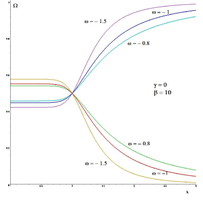
Figure 5: The decreasing functions represent the behavior of $\Omega^{(M)}$ for models with $\gamma=0$ and various choices of $\omega$. They decrease from $\Omega^{(M)}=\Omega^{(M)}_{max}=\left[1+2^{3\omega/\beta}\right]^{-1}$ at early times to $\Omega^{(M)}=0$ as $x\rightarrow\infty$ at late times. Clearly, $1/2<\Omega^{(M)}_{max}<1$ for any $\omega<0$ and $\beta>0$. Keeping $\omega$ fixed we find that $\Omega^{(M)}_{max}\rightarrow(1/2)^{+}$ for $\beta\gg 1$ and $\Omega^{(M)}_{max}\rightarrow 1^{-}$ for $\beta\rightarrow 0$. In the case under consideration, for $\beta=0$ we recover the usual CDM model with $W=\omega/2$. The increasing functions give $\Omega^{(DE)}$.

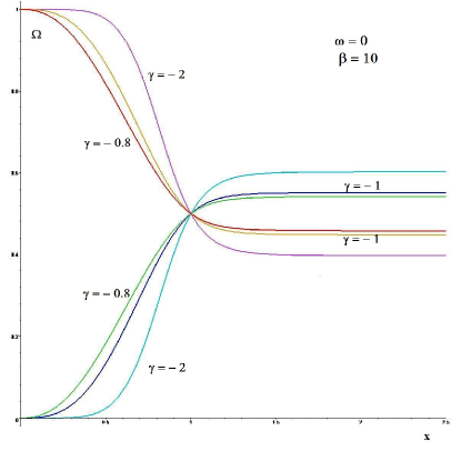
Figure 6: The decreasing functions represent the behavior of $\Omega^{(M)}$ for models with $\omega=0$ and various choices of $\gamma$. The increasing functions give $\Omega^{(DE)}$. As the universe expands $\Omega^{(M)}\rightarrow 0$ when $\omega\neq 0$. However, $\Omega^{(M)}\rightarrow\Omega^{(M)}_{min}=\left[1+2^{-3\gamma/\beta}\right]^{-1}$ when $\omega=0$. Clearly, $0<\Omega^{(M)}_{min}<1/2$ for any $\gamma<0$ and $\beta>0$. Besides, $\Omega^{(M)}_{min}\rightarrow(1/2)^{-}$ for $\beta\gg 1$ and $\Omega^{(M)}_{min}\rightarrow 0$ for $\beta\rightarrow 0$. In the case under consideration, for $\beta=0$ we recover the usual CDM model with DE characterized by a constant EoS, viz., $W=\gamma/2$.

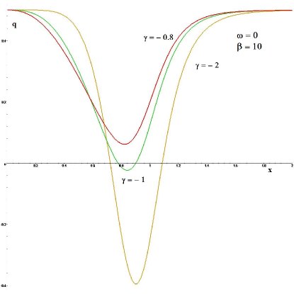
Figure 7: The figure illustrates that accelerated expansion may occur in models with $\omega=0$ for different choices of $\gamma$. The deceleration parameter has a minimum, say $q_{min}$, around the transition epoch $x=1$. For a fixed $\beta$ the minimum is negative or positive depending on $\gamma$. In the Figure $\beta=10$. For this value $q_{min}$ is negative if $\gamma<-0.943$. In general, the larger the magnitude of $\gamma$, the greater the magnitude of $q_{min}$ . Also the accelerated expansion starts earlier and finishes later with the increase of $|\gamma|$.

Chaplygin gas:

If in addition to $\gamma=0$ we set $\omega=-1$ then the energy density and pressure of the DE component satisfy the EoS (50). When $\beta$ changes in the range $3\leq\beta\leq 6$ we recover the so-called generalized Chaplygin gas. For $\beta=6$, which corresponds to the original Chapligin gas, the solution to (90) is $\bar{x}=1.069$. To obtain specific numbers for the redshifts we need to feed the equations with $\Omega_{0}^{(M)}$. The model requires $\Omega_{0}^{(M)}<2-\sqrt{2}\approx 0.586$. Thus, as an illustration we take $\Omega_{0}^{(M)}=0.3$. With this choice we find $x_{0}=1.465$, $W_{0}=-0.908$ and $q_{0}=-0.453$. The universe becomes dominated by the gas at $z_{*}=0.465$ and the phase of accelerated expansion starts at $\bar{z}=0.370$.

6.3 Solution for $\omega=0$: dark energy transforming into non-relativistic cosmic dust

Thus far we have assumed $\omega\neq 0$. Models with $\omega=0$ are diametrically opposite to the ones with $\gamma=0$. They behave as DE with $p^{(DE)}=\gamma\rho^{(DE)}$ at early times and like pressureless dust at late times. Immediately after (44), we mentioned that the replacement $\beta\rightarrow-\beta$ changes the asymptotic role of $\omega$ and $\gamma$. The solution to (89) is now given by

$$x_{0}=\left[2\left(\frac{\Omega_{0}^{(M)}}{\Omega_{0}^{(DE)}}\right)^{-\beta/3\gamma}-1\right]^{-1/\beta},$$ (95)

which can readily be obtained from (93) by replacing $\beta\rightarrow-\beta$ and $\omega\rightarrow\gamma$. However, the analogy is not complete; namely instead of (94) - with the corresponding changes - in the case under consideration the condition on $\Omega_{0}^{(M)}$ is reversed, viz.,

$$\Omega_{0}^{(M)}>\frac{1}{1+2^{-3\gamma/\beta}}.$$

Since $\beta>0$, $x_{0}\rightarrow\infty$ as $\Omega_{0}^{(M)}\rightarrow\left[1+2^{-3\gamma/\beta}\right]^{-1}$ and $q\rightarrow 1/2$ as corresponds to dust models. In Figure 6 we illustrate this for various choices of $\gamma$.

The question of whether or not this type of DE leads to an accelerated expansion depends on the choice of $\gamma$ and $\beta$. This is illustrated in Figures 7 and 8.

Reversed Chaplygin gas:

For the particular choice $\gamma=-1$ we have

$$p^{(DE)}\left[\rho^{(DE)}\right]^{\lambda}=-C_{2}^{\lambda+1},\;\;\;\;\mbox{with}\;\;\;\;\lambda=-\frac{3+\beta}{3},$$

and

$$\rho^{(DE)}=\frac{C_{2}}{\left(x^{\beta}+1\right)^{3/\beta}},\;\;\;\;p=-\frac{C_{2}}{\left(x^{\beta}+1\right)^{\left(3+\beta\right)/\beta}}.$$

For $\beta>0$, the fluid behaves like a cosmological constant for $x\ll 1$ and dust at late times. Matter dominates for small $x$ so that $q=1/2$ at early times and at late times. The expansion becomes accelerated in between for $\beta>9$. See Figures 6, 7, 8.

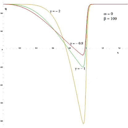
Figure 8: The figure illustrates the role of $\beta$, which measures the rapidity of transition from $\omega$ to $\gamma$. The larger $\beta$ the shorter the transition. Comparison with Figure 7 illustrates that increasing $\beta$ decreases the duration of the accelerated expansion and raises the magnitude of $q_{min}$. In this respect, the effects of $\gamma$ and $\beta$ are very much alike. This is because, when $\omega=0$, both affect the slope of $W$ in a similar way, viz., $dW/dx\sim-\gamma\beta/4$ near $x=1$.

6.4 DE acting as a cosmological constant at late times: $\omega=-1$

To obtain an explicit expression relating $\rho^{(DE)}$ and $p^{(DE)}$ we use (43) to isolate $x$ and then substitute the result into (46). To ensure that the DE behaves as a cosmological constant at late times we set $\omega=-1$. Solving for $p^{(DE)}$ we obtain

$$p^{(DE)}=\rho^{(DE)}\left[\gamma-\left(\gamma+1\right)\left(\frac{\rho^{(DE)}}{C_{2}}\right)^{-\beta/3\left(\gamma+1\right)}\right],\;\;\;\;\gamma\neq-1.$$ (96)

This can be interpreted as the superposition of two non-interacting fluids, with energy densities $\rho_{1}$ and $\rho_{2}$, evolving according to the EoS

$$p_{1}=\gamma\rho_{1},\;\;\;\;p_{2}=-A\rho^{[1-\beta/3\left(\gamma+1\right)]},$$ (97)

where $A=\left(\gamma+1\right)C_{2}^{\beta/3\left(\gamma+1\right)}$. Thus, from the continuity equation we get

$$\rho_{1}=\frac{B_{1}}{x^{3\left(1+\gamma\right)}},\;\;\;\;\rho_{2}=\left[A+\frac{B_{2}}{x^{\beta/\left(1+\gamma\right)}}\right]^{3\left(1+\gamma\right)/\beta},$$ (98)

where $B_{1}$ and $B_{2}$ are constants of integration. The above expression requires $\gamma>-1$, i.e., $A>0$, otherwise $\rho_{2}$ diverges at some finite $x\neq 0$. For $\gamma>-1$, $\rho_{1}$ acts as quintessence and $\rho_{2}$ at early times - when $x$ is small - behaves as pressureless dust: $\rho_{2}\approx 1/x^{3}$. At late times $\rho_{2}$ behaves as a cosmological term since $p_{2}=-\rho_{2}$ in that limit. For $\gamma=0$ and $\beta=6$ we have a combination of dust and Chaplygin gas.

It is well known that a scalar field $\phi$ minimally coupled to gravity with a potential $V(\phi)$ can serve as a model for DE (see e.g. [18]). In a DE-dominated universe a first order formalism gives $\left(d\phi/dx\right)^{2}=3\epsilon\left(1+W\right)/x^{2}$ and $V=\left(1-W\right)\rho/2$, where $\epsilon=1$ or $\epsilon=-1$ depending on whether $\phi$ is an ordinary scalar field ($W>-1$) or a phantom field ($W<-1$).

For $\omega=-1$ we get

$$x^{\beta}=\frac{1}{\sinh^{2}\eta\phi},\;\;\;\eta=\frac{\beta}{2\sqrt{3}\sqrt{1+\gamma}}.$$

$$V(\phi)=\frac{C_{2}}{2}\left[\left(\cosh\eta\phi\right)^{6\left(\gamma+1\right)/\beta}+\left(1-\gamma\sinh^{2}\eta\phi\right)\left(\cosh\eta\phi\right)^{2\left[3\left(\gamma+1\right)-\beta\right]/\beta}\right].$$ (99)

For $\gamma=0$ and $\beta=6$ this expression gives the potential for the Chaplygin gas discussed in [18].

6.5 DE acting as non-relativistic cosmological dust at late times: $\gamma=-1$

Following the same steps leading to (96), but this time setting $\gamma=-1$ we obtain

$$p^{(DE)}=\rho^{(DE)}\left[\omega-\left(\omega+1\right)\left(\frac{\rho^{(DE)}}{C_{2}}\right)^{\beta/3\left(\omega+1\right)}\right],\;\;\;\;\omega\neq-1.$$ (100)

Once again the DE component can be interpreted as the superposition of two non-interacting fluids, viz.,

$$p_{1}=\omega\rho_{1},\;\;\;\;\;p_{2}=-\tilde{A}\rho_{2}^{\left[1+\beta/3\left(\omega+1\right)\right]},$$

with $\tilde{A}=\left(\omega+1\right)C_{2}^{-\beta/3\left(\omega+1\right)}$ and

$$\rho_{1}=\frac{{\tilde{B}}_{1}}{x^{3\left(1+\omega\right)}},\;\;\;\;\;\rho_{2}=\frac{1}{x^{3}}\left[{\tilde{B}}_{2}+\frac{\tilde{A}}{x^{\beta/\left(1+\omega\right)}}\right]^{-3\left(1+\omega\right)/\beta},$$

where ${\tilde{B}}_{1}$ and ${\tilde{B}}_{2}$ are constants of integration, and $\tilde{A}>0$ to avoid singularities at some finite $x$. In this case the evolution of $\rho_{2}$ is diametrically opposed to that discussed in (96)-(98). Specifically, now $p_{2}=-\rho_{2}={\tilde{A}}^{-3\left(\omega+1\right)/\beta}$ at early times and $\rho_{2}\approx 1/x^{3}$ at late times. A particular example of this model is the case where $\omega=0$, which corresponds to the reversed Chaplygin gas discussed in Section $5.3$.

Following the same procedure used in the preceding subsection, we can obtain a potential by treating DE with $\gamma=-1$ as an ordinary scalar field. We find

$$x^{\beta}=\sinh^{2}{\bar{\eta}}\phi,\;\;\;\bar{\eta}=\frac{\beta}{2\sqrt{3}\sqrt{1+\omega}}.$$

and

$$V(\phi)=\frac{C_{2}}{2}\left[\left(\cosh\bar{\eta}\phi\right)^{-6\left(1+\omega\right)/\beta}+\left(1-\omega\sinh^{2}\bar{\eta}\phi\right)\left(\cosh\bar{\eta}\phi\right)^{-2\left[3\left(1+\omega\right)+\beta\right]/\beta}\right].$$ (101)

In order to avoid a possible misunderstanding, we should mention that the models with $\gamma=0$, discussed in Section $5.2$, cannot be expressed as a superposition of fluids, except in the case where $\omega=-1$. The same is true for the models with $\omega=0$ of Section $5.3$, which can be represented as a superposition of fluids only when $\gamma=-1$.

6.6 Parameter space

In the CDM models there is a simple relationship between the cosmological parameters at the current epoch. This is given by the third equation in (5). In the case under consideration, we can combine (63), with $n=0$, and (89) to eliminate $x_{0}$ and obtain a single equation, viz.,

$$\left[\frac{3\left(\gamma-\omega\right)\Omega_{0}^{(DE)}}{1-2q_{0}+3\gamma\Omega_{0}^{(DE)}}\right]^{-\gamma}\left[\frac{2q_{0}-1-3\omega\Omega_{0}^{(DE)}}{3\left(\gamma-\omega\right)\Omega_{0}^{(DE)}}\right]^{-\omega}=2^{\left(\omega-\gamma\right)}\left[\frac{\Omega_{0}^{(M)}}{\Omega_{0}^{(DE)}}\right]^{\beta/3}.$$ (102)

This replaces (5) when $\omega\neq\gamma$.

Apart from this, some general constraints on the current values of the parameters can be obtained from (63). Solving for $x^{\beta}_{0}$ we get ($\omega\neq\gamma$)

$$x^{\beta}=-\frac{3\gamma\,\Omega_{0}^{(DE)}-2q_{0}+1}{3\omega\,\Omega_{0}^{(DE)}-2q_{0}+1}.$$ (103)

For $\Omega_{0}^{(M)}<1/2$ the condition $x_{0}>1$ gives:

$\bullet$ For $\left(\omega-\gamma\right)>0$:

$$\frac{1}{2}+\frac{3}{4}\left(\gamma+\omega\right)\Omega_{0}^{(DE)}<q_{0}<\frac{1}{2}+\frac{3}{2}\omega\,\Omega_{0}^{(DE)}.$$ (104)

Accelerated expansion requires

$$\left(\omega+\gamma\right)<-\frac{2}{3\Omega_{0}^{(DE)}}.$$ (105)

Since $\omega>\gamma$, it follows that $\gamma<-1/3\Omega_{0}^{(DE)}$.

$\bullet$ For $\left(\omega-\gamma\right)<0$:

$$\frac{1}{2}+\frac{3}{2}\omega\,\Omega_{0}^{(DE)}<q_{0}<\frac{1}{2}+\frac{3}{4}\left(\gamma+\omega\right)\Omega_{0}^{(DE)}.$$ (106)

The r.h.s. part of this inequality, together with $\Omega_{0}^{(DE)}>1/2$ and $\omega<\gamma$, leads to $\gamma>-2\left(1-2q_{0}\right)/3$.

$\bullet$ It should be noted that the inequalities (104), (106) guarantee the positivity of the quantities inside the brackets in (102) for $\omega>\gamma$ and $\omega<\gamma$, respectively.

7 Summary and conclusions

Models in science perform two fundamentally different - but complementary - tasks. On the one hand, a model can indicate the type of phenomena that could actually occur in the context of the theory. On the other hand, it may shed light upon some problems of the theory.

The CDM models with $W=\omega=$ constant are important first approximations in the description of DE. They satisfactorily explain the observational data for small values of $z$, which seems to be reasonable since the equations of state of the constituents of the universe have probably not changed much in recent times. The natural question to ask is whether these models will still be useful when we have access to observations of higher values of $z$. One would expect that the details of the expansion of the universe, which are determined by the evolution of its components, will become increasingly important as we look into the past.

In this paper we have constructed a simple cosmological model which is physically reasonable, mathematically tractable, and extends the study of CDM models to the case where both the EoS for matter and DE vary with time. It is given by equations (64)-(67). The deviation from CDM models is measured by the functions $f(z)$ and $g(z)$ given by (4.3.1). For CDM models $f(z)=g(z)=1$. In our model $f(z)\approx 1$, $g(z)\approx 1$ for small $z$ and $f(z)\approx\left(1+z\right)^{3n}$, $g(z)\approx\left(1+z\right)^{-3\left(\omega-\gamma\right)}$ for large values of $z$. Consequently, the model constructed here approximates the CDM ones for small $z$ but significantly differ from them for large $z$.

We have done a thorough review of all possible cases in the whole range of parameters of the EoS (43), (53) and discussed the corresponding physical models. Some of them are quite exotic as, e.g., those with $\omega>-2/3$ and $\gamma<-2/3$ (see Table $3$) that go from decelerated to accelerated expansion, and vice versa, several times. An example is illustrated in Fig 2.

In section $5$ we investigated the effects of a primordial EoS on the present accelerated expansion. In the CDM model there is a simple relationship between the current values of the cosmological parameters $q,\omega,\Omega^{(DE)}$, which is given by (5). When $w\neq 0$ that simple equation is replaced by three inequalities, viz., (81), (85), (87) for $\Omega_{0}^{(M)}<1/2$, $\Omega_{0}^{(M)}=1/2$ and $\Omega_{0}^{(M)}>1/2$, respectively. They explicitly depend on $n$ in such a way that setting $n=0$ we recover the CDM expression (5).

We also studied the asymptotic model $\alpha\gg n$ which corresponds to the case where $w$ abruptly changes from $w=n$ to $w=0$. For $\omega\geq-2/3$ and $\Omega_{0}^{(M)}<1/2$ this and the CDM model are indistinguishable in the sense that they give the same values for $x_{0}$, $\bar{x}$, $z_{*}$ and $\bar{z}$, regardless of $n$. The situation is quite different when $\omega<-2/3$.

We note that the solutions for $\bar{x}$ sharply depend on whether DE is phantom ($\omega<-1$) or non-phantom ($\omega\geq-1$). Specifically, when the universe evolves from a radiation dominated early stage $(n=1/3)$ from the solutions (ii)-(v) of section $5.2$ we find that $\bar{x}=1$ for $-1\leq\omega<-2/3$ and $\bar{x}=\left[-\left(1+3\omega\right)/2\right]^{1/\left(3\omega-1\right)}$ for $\omega<-1$. A similar situation is seen in (5.2) where the limits on $q_{0}$ are clearly dependent on the nature of DE.

To illustrate the early and late behavior of the model, we consider the density parameter

$$\Omega^{(M)}=\frac{\left(K+1\right)^{-3n/\alpha}\left(Kx^{\alpha}+1\right)^{3n/\alpha}}{\left(K+1\right)^{-3n/\alpha}\left(Kx^{\alpha}+1\right)^{3n/\alpha}+x^{3\left(n-\gamma\right)}2^{3\left(\omega-\gamma\right)/\beta}\left(x^{\beta}+1\right)^{-3\left(\omega-\gamma\right)/\beta}}.$$

Near the origin, for small values of $x$, there are three different cases: (i) $\Omega^{(M)}=1$, (ii) $\Omega^{(M)}<1$ and (iii) $\Omega^{(M)}=0$ corresponding to $\left(n-\gamma\right)>0$, $\left(n-\gamma\right)=0$ and $\left(n-\gamma\right)<0$, respectively. The models discussed in section $5$ have $n\geq 0$ and $\omega=\gamma<0$ so they illustrate case (i). The models studied in section $6.2$, which include the generalized Chaplygin gas, have $n=\gamma=0$ so they illustrate case (ii). We have restricted our discussion to $n\geq 0$, $\gamma\leq 0$ so case (iii) has been excluded from consideration. In the limit $x\rightarrow\infty$ there are two possibilities: $\Omega^{(M)}\rightarrow 0$ and $1/2>\Omega^{(M)}>0$ for $\omega<0$ and $\omega=0$, respectively (we have not considered $\omega>0$). The models studied in section $6.3$ illustrate the second case.

In this work we have not discussed the physical mechanism leading to DE models that cross the $W=-1$ barrier. This is an important and interesting question but this is out of the scope of the present work.

References

- [1] A.G. Riess et al., Astron. J. 116 1009 (1998) [ArXiv:astro-ph/9805201].
- [2] S. Perlmutter et al., Astrophys. J. 517 565 (1999) [ArXiv:astro-ph/9812133].
- [3] R. A. Knop et al., Astrophys. J. 598 102 (2003) [ArXiv:astro-ph/0309368].
- [4] A.G. Riess et al., Astrophys. J. 607 665 (2004) [arXiv:astro-ph/0402512].
- [5] Andrew R Liddle, New Astron.Rev. 45 235 (2001) [ArXiv:astro-ph/0009491].
- [6] N. Seto, S. Kawamura and T. Nakamura, Phys.Rev.Lett. 87 221103 (2001) [ArXiv:astro-ph/0108011].
- [7] J.L. Tonry et al., Astrophys. J. 594 1 (2003) [ArXiv:astro-ph/0305008].
- [8] A.T. Lee et al, Astrophys. J. 561 L1 (2001) [ArXiv:astro-ph/0104459].
- [9] R. Stompor et al, Astrophys. J. 561 L7 (2001) [ArXiv:astro-ph/0105062].
- [10] N.W. Halverson et al, Astrophys. J. 568 38 (2002) [ArXiv:astro-ph/0104489].
- [11] C.B. Netterfield et al, Astrophys. J. 571 604 (2002) [ArXiv:astro-ph/0104460].
- [12] C. Pryke, et al., Astrophys. J. 568 46 (2002) [ArXiv:astro-ph/0104490].
- [13] D.N. Spergel et al., Astrophys. J.Suppl. 148 175 (2003) [ArXiv:astro-ph/0302209].
- [14] J. L. Sievers, et al., Astrophys. J. 591 599( 2003) [ArXiv:astro-ph/0205387].
- [15] A. Blanchard, M. Douspis, M. Rowan-Robinson and S. Sarkar, em Astron. Astrophys. 412 35 (2005).
- [16] H. Alnes, M. Amarzguioui, O. Grøn, Phys.Rev. D 73 083519 (2006) [arXiv:astro-ph/0512006].
- [17] Marie-No lle C l rier, New Advances in Physics 1 29 (2007) [arXiv:astro-ph/0702416].
- [18] E.J. Copeland, M. Sami and S. Tsujikawa, Int. J. Mod. Phys. D 15 1753 (2006) [arXiv:hep-th/0603057].
- [19] P. J. E. Peebles and B. Ratra, Rev.Mod.Phys. 75 559 (2003) [arXiv:astro-ph/0207347].
- [20] T. Padmanabhan, Phys.Rept. 380 235 (2003) [arXiv:hep-th/0212290].
- [21] I. Zlatev, L Wang and P. J. Steinhardt, Phys. Rev. Lett. 82 896 (1999) [arXiv:astro-ph/9807002].
- [22] C. Armendariz, V. Mukhanov, P. J. Steinhardt, Phys. Rev. Lett. 85 4438 (2000) [arXiv:astro-ph/0004134].
- [23] R.R. Caldwell, R. Dave, P. J. Steinhardt, Phys. Rev. Lett. 80 1592 (1998) [arXiv:astro-ph/9708069].
- [24] S.E. Deustua, R. Caldwell, P. Garnavich, L. Hui, A. Refregier, “Cosmological Parameters, Dark Energy and Large Scale Structure” [arXiv:astro-ph/0207293].
- [25] L.P. Chimento, A.S. Jakubi and D. Pavon, Phys.Rev. D 62 063508 (2000) [arXiv:astro-ph/0005070].
- [26] M. C. Bento, O. Bertolami, A. A. Sen, Phys. Rev. D 66 043507 (2002) [arXiv:gr-qc/0202064].
- [27] Zong-Kuan Guo and Yuan-Zhong Zhang, Phys. Lett. B 645 326 (2007) [arXiv:astro-ph/0506091].
- [28] C. Armendariz-Picon, V. Mukhanov and P.J. Steinhardt, Phys. Rev. Lett. 85 4438 (2000) [arXiv:astro-ph/0004134].
- [29] R. de Putter and E.V. Linder, Astropart. Phys. 28 263 (2007) [arXiv:0705.0400].
- [30] R.J. Scherrer, Phys. Rev. Lett. 93 011301 (2004) [arXiv:astro-ph/0402316].
- [31] C. Bonvin, C. Caprini and R. Durrer, Phys. Rev. Lett. 97 081303 (2006) [arXiv:astro-ph/0606584].
- [32] L. Conversi, A. Melchiorri, L. Mersini and J. Silk, Astropart. Phys. 21 443 (2004) [arXiv:astro-ph/0402529].
- [33] Gilles Esposito-Farese, Class. Quantum Grav. 25 114017 (2008) [arXiv:0711.0332].
- [34] C. Deffayet, G. R. Dvali and G. Gabadadze, Phys. Rev. D 65 044023 (2002) [arXiv:astroph/ 0105068].
- [35] G. Dvali and M. S. Turner, “Dark Energy as a Modification of the Friedmann Equation” arXiv:astro-ph/0301510.
- [36] O. Bertolami and P.J. Martins, Phys. Rev. D 61 064007 (2000) [arXiv:gr-qc/9910056].
- [37] N. Banerjee and D. Pavon, Phys. Rev. D 63 043504 (2001) [arXiv:gr-qc/0012048].
- [38] S. Sen and A. A. Sen, Phys. Rev. D 63 124006 (2001) [arXiv:gr-qc/0010092].
- [39] Hongsu Kim, Mon. Not. Roy. Astron. Soc. 364 813 (2005) [arXiv:astro-ph/0408577].
- [40] Hongsu Kim, Phys. Lett. B 606 223 (2005) [arXiv:astro-ph/0408154].
- [41] S. Das and N. Banerjee, Gen. Rel. Grav. 38 785 (2006) [arXiv:gr-qc/0507115].
- [42] W. Chakraborty and U. Debnath, Int. J. Theor. Phys. 48 232 (2009) [arXiv:0807.1776].
- [43] S. Das and N. Banerjee, Phys. Rev. D 78 043512 (2008) [arXiv:0803.3936].
- [44] Li-e Qiang, Yongge Ma, Muxin Han, Dan Yu, Phys. Rev. D 71 061501 (2005) [arXiv:gr-qc/0411066].
- [45] Li-e Qiang, Yan Gong, Yongge Ma and Xuelei Chen, “Cosmological Implications of 5-dimensional Brans-Dicke Theory” [arXiv:0910.1885].
- [46] J. Ponce de Leon, Class.Quant.Grav. 20 5321 (2003) [arXiv:gr-qc/0305041]; JCAP 03 030 (2010) [arXiv:1001.1961]; Class. Quant. Grav. 27 095002 (2010) [arXiv:0912.1026]; Int.J.Mod.Phys. D15 1237 (2006) [arXiv:gr-qc/0511150]; Gen.Rel.Grav. 38 61 (2006) [arXiv:gr-qc/0412005]; Gen.Rel.Grav. 37 53 (2005) [arXiv:gr-qc/0401026].
- [47] S. Hannestad and E. Mörtsell, JCAP 0409 001 (2004) arXiv:astro-ph/0407259.
- [48] H, Štefancic, Phys. Rev. D 71 124036 (2005).
- [49] V. Sahni, T.D. Saini, A.A. Starobinsky, and U. Alam, JETP Lett. 77 201 (2003) [arXiv:astro-ph/0201498].
- [50] U. Alam, V. Sahni, T.D. Saini, and A.A. Starobinsky, Mon. Not. Roy. Astr. Soc. 344 1057 (2003) [arXiv:astro-ph/0303009].
- [51] M. Israelit and N. Rosen, Astrophys. J. 342 627 (1989).
- [52] M. Israelit and N. Rosen, Astrophys. Space Sci. 204 317 (1993).