Magnetic Impurities in Two-Dimensional Superfluid Fermi Gas
with Spin-Orbit Coupling

Abstract

We consider magnetic impurities in a two dimensional superfluid Fermi gas in the presence of spin-orbit coupling. By using the methods of t-matrix and Green’s function, we find spin-orbit coupling has some dramatic impacts on the effects of magnetic impurities. For the single impurity problem, the number of bound states localized around the magnetic impurity is doubled. For the finite concentration $n$ of impurities, the energy gap is reduced and the density of states in the gapless region is greatly modified.

I Introduction

In the last few years, topological insulator (TI) and topological superconductor (TSC) M. Z. Hasan ; X. L. Qi have arisen a lasting interest in condensed matter systems. In such systems, spin-orbit coupling plays a fundamental role to make the TI and TSC different from the traditional insulator and traditional BCS superconductor significantly. In cold atomic field, the superfluid of Fermi gases have been realized in ${{}^{40}}K$ C. A. Regal and ${{}^{6}}Li$ M. Bartenstein ; M. W. Zwierlein ; J. Kinast , furthermore, spin-orbit coupling has also been realized by the more recent experimental achievement of synthetic gauge field Y. -J. Lin1 ; Y. -J. Lin2 . By Introducing the effect of spin-orbit coupling, new phases analog to TSC and new phenomena may emerge in cold superfluid Fermi gases, e.g. topological superfluid and topological phase-separation Xiaosen Yang . Since a cold atomic system is more adjustable, it can provide a more controllable way to study such phases under different conditions, e.g. magnetic impurities.

From TI and TSC, we know that spin-orbit coupling combining with Zeeman field greatly change the energy spectrum and make topological phases emerge. Therefore, to figure out how the spin-orbit coupling affects the effect of magnetic impurity, which likes a local magnetic moment, is a very interesting problem. Recently, people have paid attention to studying on the Kondo effect in the presence of spin-orbit coupling Rok Zitko ; Mahdi Zarea ; L. Isaev , however, in this paper, we will study the effects of classical magnetic impurity in superfluid Fermi gases in the presence of spin-orbit coupling. Since cold Fermi gas system is much cleaner than metallic superconductor and the strength of pairing interaction can be tuned by adjusting the threshold energy of Feshbach resonance, obviously, it’s a better platform to detect the effects of dilute magnetic impurities.

The effects of magnetic impurities are particularly important in the case of superconductor, and so superfluidity. Magnetic impurities which can flip the spins of electrons interfere with the pairing and reduce the gap. A sufficient concentration of magnetic impurities leads to gapless superconductivity, where the superconductive order parameter still exist but the BCS excitation gap is absent A. A. Abrikosov ; K. Maki . Such a pairing-breaking effect is absent in the case of nonmagnetic impurities (known as Anderson’s theorem), so in the following, we only consider the effects of magnetic impurities.

In this paper, we discuss the effects of magnetic impurities in a two dimensional superfluid Fermi gas in the presence of spin-orbit coupling. So far, nonmagnetic impurities have been realized in Bose gases by using other species of atoms C. Zipkes and laser light G. Modugno . Recently, a single spin-$\downarrow$ placed in a Fermi sea of spin-$\uparrow$ atoms is observed to behave as a mobile impurity to form Fermi polaron A. Schirotzek ; S. Nascimbene . To realize magnetic impurities in a superfluid Fermi gas, Y. Ohashi Y. Ohashi suggests and confirms that nonmagnetic impurities accompanied by localized spin-$\uparrow$ can be viewed as magnetic impurities. Based on these, we believe it is not far away to detect the effects of magnetic impurities in a superfluid Fermi gas with spin-orbit coupling in real experiments.

The paper is organized as follows. In Sec.II, we consider the case of single magnetic impurity and calculate the energy of bound state in the presence of spin-orbit coupling. In Sec.III, we generalize the single impurity case to the one of concentration $n$. In Sec.IV, a conclusion is given.

II Single Impurity Model

Now, we consider a two dimensional ultra-cold atomic system with single magnetic impurity and spin-orbit coupling, which is described by

$$H = H_{0}+H_{imp},$$

$$H_{0} = \sum_{k\sigma}\varepsilon_{k}c_{k\sigma}^{{\dagger}}c_{k\sigma}+\sum_{k}\alpha_{R}k\left(e^{i\varphi_{k}}c_{k\uparrow}^{{\dagger}}c_{k\downarrow}+e^{-i\varphi_{k}}c_{k\downarrow}^{{\dagger}}c_{k\uparrow}\right)$$

$$-\Delta\sum_{k}\left(c_{k\uparrow}^{{\dagger}}c_{-k\downarrow}^{{\dagger}}+c_{-k\downarrow}c_{k\uparrow}\right),$$

$$H_{imp} = \frac{U}{2}s_{z}\sum_{k,k^{{}^{\prime}},\sigma}c_{k\sigma}^{{\dagger}}\sigma c_{k^{{}^{\prime}}\sigma},$$ (1)

where $\varepsilon_{k}=k^{2}/2m-\mu$, $\alpha_{R}$ is the strength of spin-orbit coupling, $c_{k\sigma}^{{\dagger}}(c_{k\sigma})$ is creation(annihilation) operator with pseudo-spin $\sigma$, $\Delta$ is the order parameter, $U$ is the on-site interaction strength and $s_{z}=\pm s$ is the number of excess spin-up atoms localized around impurity (see Refs.Y. Ohashi ). For simplicity, here we completely neglect the effect of the local spatial variation of the order parameter around a paramagnetic impurity.

In the Nambu spinor presentation $\Psi_{k}^{{\dagger}}=(c_{k\uparrow}^{{\dagger}},c_{k\downarrow}^{{\dagger}},c_{-k\downarrow},c_{-k\uparrow})$, $H_{0}$ can be rewritten as

$$H_{0} = \frac{1}{2}\sum_{k}\Psi_{k}^{{\dagger}}H(k)\Psi_{k},$$

$$H(k) = \varepsilon_{k}\tau_{3}-\Delta\rho_{1}\tau_{3}+\alpha_{R}k\left(e^{i\varphi_{k}}\tau_{+}+e^{-i\varphi_{k}}\tau_{-}\right),$$ (2)

where $\rho_{i}$ and $\tau_{i}(i=1,2,3)$ are Pauli matrices in particle-hole space and spin space, respectively, and $\tau_{\pm}=(\tau_{1}\pm i\tau_{2})/2$. According to Ref.H. Shiba or the method of the coherent state path integral Alexander Altland , we can have

$$G_{0}(k,\omega)=\frac{1}{\omega-\varepsilon_{k}\tau_{3}+\Delta\rho_{1}\tau_{3}-\alpha_{R}k(e^{i\varphi_{k}}\tau_{+}+e^{-i\varphi_{k}}\tau_{-})},$$

(3)

$G_{0}(k,\omega)$ is related to the full Green function $G(k,\omega)$ in the following form

$$G(k,k^{{}^{\prime}},\omega)=G_{0}(k,\omega)\delta_{kk^{{}^{\prime}}}+G_{0}(k,\omega)t(\omega)G_{0}(k^{{}^{\prime}},\omega).$$ (4)

After averaging over the direction of the spin, the non-flip part of the t-matrix, $t(\omega)$, is given by

$$t(\omega)=\frac{(\frac{U}{2}s)^{2}F(\omega)}{1-(\frac{U}{2}s)^{2}F(\omega)^{2}},$$ (5)

where $F(\omega)$ is

$$F(\omega)=\sum_{k}G_{0}(k,\omega).$$ (6)

We are interested in the localized excited state in the energy gap $\Delta$, so we must find poles of $t(\omega)$. For $|\omega|<\Delta$, by integrating out $k$ in Eq.(6) (see details in Appendix), we obtain

$$F(\omega)=-\pi\rho(0)\frac{\omega-\Delta\rho_{1}\tau_{3}-m\alpha_{R}^{2}\rho_{3}}{\sqrt{\Delta^{2}-\omega^{2}}},$$ (7)

where $\rho(0)$ is the density of states at the Fermi level in the normal state. Based on Eqs.(5) and (7), the poles of $t(\omega)$ are given by (see details in Appendix)

$$\omega_{1} = \pm\left(1-\frac{1}{8}A\frac{m^{4}\alpha_{R}^{8}}{\Delta^{4}}\right)\Delta,$$

$$\omega_{2} = \pm\left(\frac{1-A}{1+A}-\frac{A}{1+A}\frac{m^{2}\alpha_{R}^{4}}{\Delta^{2}}\right)\Delta,$$ (8)

where $A=(Us\pi\rho(0)/2)^{2}$. From Eq.(8), it’s easy to see, no matter how small $A$ may be, two bound states always appear, this result is quite different from the case in the absence of spin-orbit coupling. However, for $\alpha_{R}=0$, there are only two poles in the energy gap, and the poles reduce to $\omega=\pm[(1-A)/(1+A)]\Delta$, just the same result as in Refs.H. Shiba ; Y. Ohashi ; Lei Jiang . Increasing the strength of spin-orbit coupling, the energy of the low-lying state which is localized around the impurity goes to zero. From Eq.(8), we can see, if we increase the strength of $U$ and keep $A<1$, the combined effects of magnetic impurity and spin-orbit coupling is strengthened, and the energy of the bound state will go to zero faster than the case in the absence of spin-orbit coupling.

III Impurity of Concentration n

Now, we generalize single impurity to the case for finite concentration n. After averaging over the random distribution of the impurities, the Green’s function recovers the translational invariance, and the renormalized Green’s function is given by

$$G(k,\omega)=\frac{1}{\tilde{\omega}-\varepsilon_{k}\tau_{3}+\tilde{\Delta}\rho_{1}\tau_{3}-\alpha_{R}k(e^{i\varphi_{k}}\tau_{+}+e^{-i\varphi_{k}}\tau_{-})},$$

(9)

where $\tilde{\omega}$ and $\tilde{\Delta}$ are the renormalized frequency and order parameter, respectively. $\tilde{\omega}$ and $\tilde{\Delta}$ are determined by Dyson equation

$$G(k,\omega)=G_{0}(k,\omega)+G_{0}(k,\omega)\Sigma(k,\omega)G(k,\omega),$$ (10)

another useful form of this formula is

$$G(k,\omega)^{-1}=G_{0}(k,\omega)^{-1}-\Sigma(k,\omega),$$ (11)

where $G_{0}(k,\omega)$, the Green’s function in the absence of impurities, is given by Eq.(3). In Born approximation, the self energy $\Sigma(k,\omega)$ is given by K. Maki

$$\Sigma(k,\omega)=-\frac{1}{2\tau_{s}}\frac{\tilde{\omega}-\tilde{\Delta}\rho_{1}\tau_{3}-m\alpha_{R}^{2}\rho_{3}}{\sqrt{\tilde{\Delta}^{2}-\tilde{\omega}^{2}}},$$ (12)

where $\tau_{s}$ is the relaxation time and is given by

$$\tau_{s}=\pi\rho(0)ns^{2}U^{2}.$$ (13)

By substituting Eq.(12) into Eq.(11), we obtain

$$\tilde{\omega}_{1} = \omega_{1}+\frac{1}{2\tau_{s}}\frac{\tilde{\omega}_{1}+m\alpha_{R}^{2}}{\sqrt{\tilde{\Delta}_{1}^{2}-\tilde{\omega}_{1}^{2}}},$$

$$\tilde{\Delta}_{1} = \Delta_{1}-\frac{1}{2\tau_{s}}\frac{\tilde{\Delta}_{1}}{\sqrt{\tilde{\Delta}_{1}^{2}-\tilde{\omega}_{1}^{2}}},$$ (14)

and

$$\tilde{\omega}_{2} = \omega_{2}+\frac{1}{2\tau_{s}}\frac{\tilde{\omega}_{2}-m\alpha_{R}^{2}}{\sqrt{\tilde{\Delta}_{2}^{2}-\tilde{\omega}_{2}^{2}}},$$

$$\tilde{\Delta}_{2} = \Delta_{2}-\frac{1}{2\tau_{s}}\frac{\tilde{\Delta}_{2}}{\sqrt{\tilde{\Delta}_{2}^{2}-\tilde{\omega}_{2}^{2}}},$$ (15)

where $\Delta_{1}=\Delta_{2}=\Delta$. They are quite different from the case without spin-orbit coupling, as before, with spin-orbit coupling, the number of poles of t-matrix has increased from two to four. By introducing a new auxiliary parameter $u_{i}$ defined by $u_{i}\equiv\tilde{\omega}_{i}/\tilde{\Delta}_{i}$ $(i=1,2)$, Eqs.(14)-(15) are reduced as

$$\frac{\omega_{i}}{\Delta_{i}} = u_{i}\left(1-\zeta_{i}\frac{1}{\sqrt{1-u_{i}^{2}}}\right)+(-1)^{i}v_{i}\frac{\zeta_{i}}{2\sqrt{1-u_{i}^{2}}-\zeta_{i}},$$

$$\zeta_{i} = \frac{1}{\tau_{s}\Delta_{i}},~{}~{}~{}~{}~{}~{}v_{i}=\frac{m\alpha_{R}^{2}}{\Delta_{i}}.$$ (16)

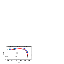
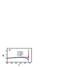
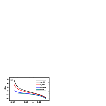
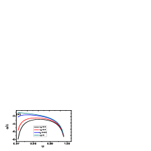
Figure 1: (Color online) The parameters of Eq.(16) are: $\zeta=0.5$. The values of $v_{i}$ are shown in the figure. (a) There is a maximum for every fixed $v_{1}$, and the value of the maximum decreases monotonically with $v_{1}$. (b) There is no maximum, when $u$ goes to the critical value $u_{c}$, the value of $\omega/\Delta$ diverges. (c) When $u\in(u_{c},1)$, $\omega/\Delta$ decreases with $u$ monotonically. (d) There is a maximum for every fixed non zero $v_{2}$, and the value of the maximum decreases monotonically with $v_{2}$

Plotting the above equation in the $u\omega$-plane (as shown in Fig.1), we can see the case in the absence of spin-orbit coupling is quite different from the one with spin-orbit coupling.

First, for $\zeta<2$ case, with the spin-orbit coupling, there are two poles in Eq.(16), one is at $u_{c}=\sqrt{1-\zeta^{2}/4}$, and the other is the original one at $u_{c}=1$. In the absence of spin-orbit coupling, for $v=0$, $\omega$ goes through a maximum and afterwards decrease monotonically, this is also the characteristic of Fig.1(a)(c)(d). However, there is no such characteristic in Fig.1(b), after $\omega$ goes through a finite maximum, $\omega$ will not decreases monotonically, in the opposite, when $u$ goes to $u_{c}$, $\omega$ is positive and diverges. So only the maximum value of $\omega$ in Fig.1(a) has the meaning of the energy gap $\omega_{g}$ (in the following, we only consider this case). It is determined by the condition

$$\frac{1}{\Delta}\frac{\partial\omega}{\partial u} = 1-\zeta(1-u^{2})^{-3/2}-\frac{2vu\zeta}{\sqrt{1-u^{2}}(2\sqrt{1-u^{2}}-\zeta)^{2}}$$ (17)

$$= 0.$$

This equation is difficult to solve. However, by numerical calculating, we find that if $v$ be sufficiently small, like $v=0.05$ in Fig.1, we can safely ignore the last term in Eq.(17) (see Fig.2), and obtain

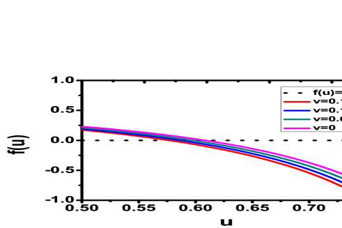
Figure 2: (Color online) The parameters of Eq.(17) are: $\zeta=0.5$. $f(u)=\frac{1}{\Delta}\frac{\partial\omega}{\partial u}$. By increasing $v$ from $v=0.05$ to $v=0.15$, $u_{0}$, the $u$ corresponds to the maximum of $\frac{\omega}{\Delta}$, changes slowly.

$$u_{0} \simeq (1-\zeta^{2/3})^{1/2},$$

$$\omega_{g} \simeq \Delta\left[(1-\zeta^{2/3})^{3/2}+\frac{v}{1-2\zeta^{-2/3}}\right].$$ (18)

We see that the solution of Eq.(17) exist only when $\zeta<1$. In fact, even we consider the effect of spin-orbit coupling and modify $u_{0}$ to $(1-a-\zeta^{2/3})^{1/2}$, to first order, the expression of $\omega_{g}$ in Eq.(16) will not change. Based on above, we can expand Eq.(16) around $u_{0}$ and obtain

$$\frac{\omega-\omega_{g}}{\Delta}=-\frac{3}{2}\zeta^{-\frac{2}{3}}\left[(1-\zeta^{\frac{2}{3}})^{\frac{1}{2}}+\frac{v(8-6\zeta^{\frac{2}{3}})}{3(2-\zeta^{\frac{2}{3}})^{3}}\right](u-u_{0})^{2}.$$

(19)

Second, for $1<\zeta<2$ case, $\omega$ decreases monotonically as $u$ increases between $[0,u_{c})$. This corresponds to $\omega_{g}=0$. Because of the presence of spin-orbit coupling, from Eq.(18), we can see that, when $\zeta<1$, $\omega_{g}$ can reach zero. This indicates that spin-orbit coupling modifies strongly the critical concentration $n_{c}$ ( $n_{c}$ corresponds to $\zeta=1$ in the absence of spin-orbit coupling), where the gap in the energy spectrum $\omega_{g}$ vanishes and the gapless superfluidity appears.

For small values of $\omega$, an asymptotic expression of $u$ based on Eq.(15) is given by

$$u= i\sqrt{(\zeta+\alpha)^{2}-1}$$ (20)

$$+\left[1-\frac{\xi}{(\zeta+\alpha)^{3}}-\frac{2vi\zeta\sqrt{(\zeta+\alpha)^{2}-1}}{(\zeta+\alpha)(\zeta+2\alpha)^{2}}\right]^{-1}\frac{\omega}{\Delta}$$

$$+...,$$

where $\alpha$ is a small constant determined by

$$i\frac{\alpha}{\zeta+\alpha}\sqrt{(\zeta+\alpha)^{2}-1}=\frac{v\zeta}{\zeta+2\alpha}.$$ (21)

For sufficiently small $v$, $\alpha$ can be ignored, and Eq.(20) can be reduced as

$$u= i\sqrt{\zeta^{2}-1}$$ (22)

$$+\zeta^{2}\left(\zeta^{2}-1-2iv\sqrt{\zeta^{2}-1}\right)^{-1}\frac{\omega}{\Delta}$$

$$+...$$

In the following, in order to show what are changed by the spin-orbit coupling, we calculate the density of states, which can be measured by STM. The density of states is given in terms of the Green’s function by

$$N_{S}(\omega) = \frac{1}{2\pi}\text{Im}\int\frac{d^{2}k}{(2\pi)^{2}}\text{Tr}[G(k,\omega)]$$ (23)

$$= N_{0}\text{Im}\left(\frac{\tilde{\omega}}{\sqrt{\tilde{\Delta}^{2}-\tilde{\omega}^{2}}}\right)$$

$$= N(0)\text{Im}\left(\frac{u}{\sqrt{1-u^{2}}}\right).$$

Making use of Eq.(16) (here we can also safely ignore the last term), the above formula reduces to a more convenient form:

$$N_{S}(\omega)=N(0)\zeta^{-1}\text{Im}u.$$ (24)

First, let us consider $\zeta<1$ case, by using Eq.(19), we substitute the expression of $u$ into Eq.(24) and obtain

$$N_{S}(\omega) = \left\{\begin{aligned} &0&\omega<\omega_{g}\\ &N(0)\zeta^{-\frac{2}{3}}B^{-\frac{1}{2}}\sqrt{\frac{2(\omega-\omega_{g})}{3\Delta}}&\omega\geq\omega_{g}\\ \end{aligned}\right.,$$

$$B = (1-\zeta^{\frac{2}{3}})^{\frac{1}{2}}+\frac{v(8-6\zeta^{\frac{2}{3}})}{3(2-\zeta^{\frac{2}{3}})^{3}}.$$ (25)

From Eq.(25), we see that $\omega_{g}$ gives the threshold frequency of the density of states, and spin-orbit coupling reduces the value of $N_{S}(\omega)$ for $\omega>\omega_{g}$. This is obviously right, since from Eq.(18), we see spin-orbit coupling reduces the value of $\omega_{g}$. To guarantee $\int N_{s}(\omega)d\omega$ invariant, the reduction of $N_{S}(\omega)$ is necessary.

Second, for $\zeta>1$ case, by Eq.(22) we obtain

$$N_{S}(\omega) = N(0)[(1-\zeta^{-2})^{\frac{1}{2}}+\frac{2v\zeta}{\sqrt{\zeta^{2}-1}[4v^{2}+(\zeta^{2}-1)]}\frac{\omega}{\Delta}$$

$$+ \frac{\zeta[3+2v(\zeta^{2}-5)][(\zeta^{2}-1)^{2}-4v^{2}(\zeta^{2}-1)]}{2\sqrt{\zeta^{2}-1}[(\zeta^{2}-1)^{2}+4v^{2}(\zeta^{2}-1)]^{2}}](\frac{\omega}{\Delta})^{2},$$

here we have reconsidered the second order of $\omega/\Delta$. From Eq.(LABEL:27), we can see $N_{s}$ is finite at $\omega=0$ and given by $N_{S}(0)=(1-\zeta^{-2})^{1/2}N(0)$. This is just a characteristic of the gapless region, where the energy spectrum $\omega_{g}$ vanishes though the gap parameter $\Delta$ is not zero. This is an example of gapless superfluidity, the existence of Cooper pairs without the existence of an energy gap in the spectrum of excitations.

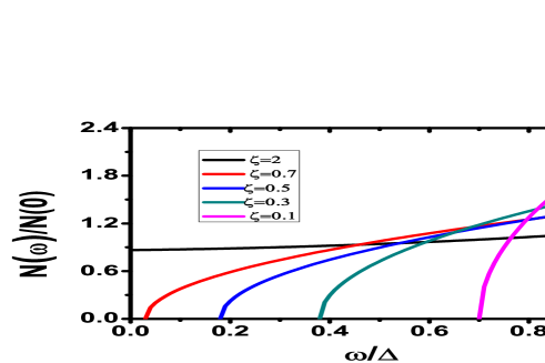
Figure 3: (Color online) Density of states plotted for different values of $\zeta$. The parameter $v$ is set to 0.1.

From Eq.(LABEL:27), we also find that, for $\omega/\Delta$ sufficiently small, $N_{S}(\omega)\propto\omega$, which is quite different from $N_{S}(\omega)\propto\omega^{2}$ in the absence of spin-orbit coupling K. Maki . From all of the above, it’s obviously that the spin-orbit coupling affects the effects of magnetic impurities a lot.

IV Conclusions

In this paper, we have investigated the effects of magnetic impurities in a two-dimensional superfluid Fermi gas with spin-orbit coupling. In the presence of spin-orbit coupling, by using the methods of t-matrix, we find that the number of bound states has doubled comparing to the case without spin-orbit coupling. By using the methods of Green’s function, we also find that the spin-orbit coupling changes the energy gap in the energy spectrum and density of states. In the gap region, the larger the concentration, the stronger the impact is given by the spin-orbit coupling. In the gapless region (here limited to $\zeta>1$), we find spin-orbit coupling changes the relation between $N(\omega)$ and $\omega$ from $N(\omega)\propto\omega^{2}$ to $N(\omega)\propto\omega$ in the small $\omega$ limit.

Since we only consider the spin-flip effects of the magnetic impurities and totally ignore the spin-exchange effects, the impurities are classical impurities and as a result, the Kondo effect is absent. In future, such a system including spin-exchange term may be used to explore the effects of spin-orbit coupling to the Kondo problem in cold atomic systems. In addition, the effects of magnetic impurities in imbalance Fermi gas with spin-orbit coupling are also worth exploring.

Appendix A Appendix

To obtain Eq.(7), we first write down the Green’s function in the absence of a magnetic impurity,

$$G_{0}(k,\omega)=\frac{1}{\omega-\varepsilon_{k}\tau_{3}+\Delta\rho_{1}\tau_{3}-\alpha_{R}k(e^{i\varphi_{k}}\tau_{+}+e^{-i\varphi_{k}}\tau_{-})},$$

$G_{0}(k,\omega)$ is a $4\times 4$ matrix, after we write down its entities, by using the formula

$$F(\omega)=\sum_{k}G_{0}(k,\omega),$$ (28)

we can integrate out $k$ directly, and obtain the entities of $F(\omega)$. However, because the presence of spin-orbit coupling, the energy spectrum has greatly modified, and this makes the integration difficult. To avoid this difficulty, we assume the strength of spin-orbit coupling, $\alpha_{R}<<V_{F}$, where $V_{F}=k_{F}/m$ is the Fermi velocity. Following the assumption $k-k_{F}\approx m\epsilon/k_{F}$ made by G. Rickayzen when he solved the problem of impurities in metalG. Rickayzen , assuming the particle-hole symmetry of Fermi band and approximating the normal-state density of states by the value $\rho(0)$ at the Fermi level, we obtain

$$F(\omega)=-\pi\rho(0)\frac{\omega-\Delta\rho_{1}\tau_{3}-m\alpha_{R}^{2}\rho_{3}}{\sqrt{\Delta^{2}-\omega^{2}}}.$$ (29)

Using this formula and Eq.(5), we obtain the equation for the bound-state energies as

$$0=\text{det}[1-AF(\omega)^{2}],$$ (30)

where $A=(Us\pi\rho(0)/2)^{2}$. By directly solving a eigenvalue problem and assuming $m\alpha_{R}^{2}/\Delta<<1$, we obtain

$$\omega_{1} = \pm(1-\frac{1}{8}A\frac{m^{4}\alpha_{R}^{8}}{\Delta^{4}})\Delta,$$

$$\omega_{2} = \pm(\frac{1-A}{1+A}-\frac{A}{1+A}\frac{m^{2}\alpha_{R}^{4}}{\Delta^{2}})\Delta.$$ (31)

References

- (1) M. Z. Hasan, C. L. Kane, Rev. Mod. Phys. 82, 3045 (2010).
- (2) X. L. Qi, S. C. Zhang, Rev. Mod. Phys. 83, 1057 (2011)
- (3) C. A. Regal, M. Greiner, and D. S. Jin, Phys. Rev. Lett. 92, 040403 (2004)
- (4) M. Bartenstein, A. Altmeyer, S. Riedl, S. Jochim, C. Chin, J. H. Denschlag, and R. Grimm, Phys. Rev. Lett. 92, 120401 (2004)
- (5) M. W. Zwierlein, C. A. Stan, C. H. Schunck, S. M. F. Raupach, A. J. Kerman, and W. Ketterle, Phys. Rev. Lett. 92, 120403 (2004)
- (6) J. Kinast, S. L. Hemmer, M. E. Gehm, A. Turlpov, and J. E. Thomas, Phys. Rev. Lett. 92, 150402 (2004)
- (7) Y. -J. Lin, R. L. Compton, A. R. Perry, W. D. Phillips, J. V. Porto, and I. B. Spielman, phys. Rev. Lett. 102, 130401 (2009)
- (8) Y. -J. Lin, K.Jimenez-Garcia, and I. B. Spielman, Nature 471, 83 (2011).
- (9) Xiaosen Yang, Shaolong Wan, Phys. Rev. A 85, 023633 (2012).
- (10) Rok Zitko and Janez Bonca, Phys. Rev. B 84, 193411 (2011).
- (11) Mahdi Zarea, Sergio E. Ulloa, and Nancy Sandler, Phys. Rev. Lett. 108, 046601 (2012)
- (12) L. Isaev, D. F. Agterberg, and I. Vekhter, Phys. Rev. B 85, 081107 (2012)
- (13) A. A. Abrikosov and L. P. Gor’kov, Sov. Phys. JETP 15, 752(1962).
- (14) K. Maki, in , edited by R. D. Parks (Marcel Dekker, New York, 1969),p1045-1046.
- (15) C. Zipkes, S. Palzer, C. Sias, and M. K ohl, Nature (London) 464, 388 (2010).
- (16) G. Modugno, Rep. Prog. Phys. 73, 102401 (2010).
- (17) A. Schirotzek, C. H. Wu, A. Sommer, and M. W. Zwierlein, Phys. Rev. Lett. 102, 230402 (2009).
- (18) S. Nascimbene, N. Navon, K. J. Jiang, L. Tarruell, M. Teichmann, J. McKeever, F. Chevy, and C. Salomon, Phys. Rev. Lett. 103, 170402 (2009).
- (19) Y. Ohashi, Phys. Rev. A 83,063611 (2011).
- (20) H. Shiba, Prog. Theor. Phys. 40, 435 (1968).
- (21) Alexander Altland and Ben Simons, , Chap.6. Cambridge Univ. Press (2006).
- (22) Lei Jiang, Leslie O. Baksmaty, Hui Hu, Yan Chen, and Han pu, Phys. Rev. A 83 061604 (2011)
- (23) G. Rickayzen, , Chap.4. Academic Press (1980).