A space-time smooth artificial viscosity method for nonlinear conservation laws

Abstract

We introduce a new methodology for adding localized, space-time smooth, artificial viscosity to nonlinear systems of conservation laws which propagate shock waves, rarefactions, and contact discontinuities, which we call the $C$-method. We shall focus our attention on the compressible Euler equations in one space dimension. The novel feature of our approach involves the coupling of a linear scalar reaction-diffusion equation to our system of conservation laws, whose solution $C(x,t)$ is the coefficient to an additional (and artificial) term added to the flux, which determines the location, localization, and strength of the artificial viscosity. Near shock discontinuities, $C(x,t)$ is large and localized, and transitions smoothly in space-time to zero away from discontinuities. Our approach is a provably convergent, spacetime-regularized variant of the original idea of Richtmeyer and Von Neumann, and is provided at the level of the PDE, thus allowing a host of numerical discretization schemes to be employed.

We demonstrate the effectiveness of the $C$-method with three different numerical implementations and apply these to a collection of classical problems: the Sod shock-tube, the Osher-Shu shock-tube, the Woodward-Colella blast wave and the Leblanc shock-tube. First, we use a classical continuous finite-element implementation using second-order discretization in both space and time , FEM-C. Second, we use a simplified WENO scheme within our $C$-method framework, WENO-C. Third, we use WENO with the Lax-Friedrichs flux together with the $C$-equation, and call this WENO-LF-C. All three schemes yield higher-order discretization strategies, which provide sharp shock resolution with minimal overshoot and noise, and compare well with higher-order WENO schemes that employ approximate Riemann solvers, outperforming them for the difficult Leblanc shock tube experiment.

1 Introduction

1.1 Smoothing conservation laws

The initial-value problem for a general nonlinear system of conservation laws can be written as an evolution equation,

$$\partial_{t}U(x,t)+\operatorname{div}F(U(x,t))=0\text{ with }U|_{t=0}=U_{0}\,,$$ (1)

for an $m$-vector $U$ defined on ($D$$+$$1$)-dimensional space-time. Such partial differential equations (PDE) are both ubiquitous and fundamental in science and engineering, and include the compressible Euler equations of gas dynamics, the magneto-hydrodynamic (MHD) equations modeling ionized plasma, the elasticity equations of solid mechanics, and numerous related physical systems which possess complicated nonlinear wave interactions.

It is well known that solutions of (1) can develop finite-time shocks, even when the initial data is smooth, in which case, discontinuities of $U$ are propagated according to the so-called Rankine-Hugoniot conditions (see Section 2.1 below). It is important to develop stable and robust numerical algorithms which can approximate weak shock-wave solutions. Even in one-space dimension, nonlinear wave interaction such as two shock waves colliding, is a difficult problem when considering accuracy, stability and monotonicity. The challenge is maintaining higher-order accuracy away from the shock while approximating the discontinuity in an order-$\Delta x$ smooth transition region where $\Delta x$ denotes the spatial grid size.

As we describe below, a variety of clever discretization schemes have been developed and employed, particularly in one-space dimension, to approximate discontinuous solution profiles in an essentially non-oscillatory (ENO) fashion. These include, but are not limited to, total variation diminishing (TVD) schemes, flux-corrected transport (FCT) schemes, weighted essentially non-oscillatory (WENO) schemes, discontinuous Galerkin methods, artificial diffusion methods, exact and approximate Riemann solvers, and a host of variants and combinations of these techniques.

We develop a robust parabolic-type regularization of (1), which we refer to as the $C$-method, which couples a modified set of $m$ equations for $U$ with an additional linear scalar reaction-diffusion equation for a new scalar field $C(x,t)$. Thus, instead of (1) we consider a system of $m$$+$$1$ equations, which use the solution $C(x,t)$ as a coefficient in a carefully chosen modification of the flux. As we describe in detail below, the solution $C(x,t)$ is highly localized in regions of discontinuity, and transitions smoothly (in both $x$ and $t$) to zero in regions wherein the solution is smooth. Further, as $\Delta x\to 0$, we recover the original hyperbolic nonlinear system of conservation laws (1).

1.2 Numerical discretization

In the case of 1-D gas dynamics, the construction of non-oscillatory, higher-order, numerical algorithms such as ENO by Harten, Engquist, Osher & Chakravarthy [1] and Shu & Osher [2], [3]; WENO by Liu, Osher, & Chan [4] and Jiang & Shu [5]; MUSCL by Van Leer [6], Colella [7], and Huynh [8]; or PPM by Colella & Woodward [9] requires carefully chosen reconstruction and numerical flux.

Such numerical methods evolve cell-averaged quantities; to calculate an accurate approximation of the flux at cell-interfaces, these schemes reconstruct $k$th-order ($k\geq 2$) polynomial approximations of the solution (and hence the flux) from the computed cell-averages, and thus provide $k$th-order accuracy away from discontinuities. See, for example, the convergence plots of Greenough & Rider [10] and Liska & Wendroff [11]. Given a polynomial representation of the solution, a strategy is chosen to compute the most accurate cell-interface flux, and this is achieved by a variety of algorithms. Centered numerical fluxes, such as Lax-Friedrichs, add dissipation as a mechanism to preserve stability and monotonicity. On the other hand, characteristic-type upwinding based upon exact (Godunov) or approximate (Roe, Osher, HLL, HLLC) Riemann solvers, which preserve monotonicity without adding too much dissipation, tend to be rather complex and PDE-specific; moreover, for strong shocks, other techniques may be required to dampen post-shock oscillations or to yield entropy-satisfying approximations (see Quirk [12]). Again, we refer the reader to the papers [10], [11] or Colella & Woodward [13] for a thorough overview, as well as a comparison of the effectiveness of a variety of competitive schemes.

Majda & Osher [14] have shown that any numerical scheme is at best, first-order accurate in the presence of shocks or discontinuities. The use of higher-order numerical schemes is, nevertheless, imperative for the elimination of error-terms in the Taylor expansion (in mesh-size) and the subsequent limiting of truncation error. Moreover, higher-order schemes tend to be less dissipative than there lower-order counterparts, as discussed by Greenough & Rider [10]; therein, a comparison between a $2$nd-order PLMDE scheme and a $5$th-order WENO scheme demonstrates the improved resolution of intricate fine structure afforded by $5$th-order WENO, while simultaneously providing far less clipping of local extrema than PLMDE.

In multi-D, similar tools are required to obtain non-oscillatory numerical schemes, but the multi-dimensional analogues to those described above are generally limited by mesh considerations. For structured grids (such as products of uniform 1-D grids), dimensional splitting is commonly used, decomposing the problem into a sequence of 1-D problems. This technique is quite successful, but stringent mesh requirements prohibits its use on complex domains. Moreover, applications to PDE outside of variants of the Euler equations may be somewhat limited. For further discussion of the limitations of dimensional splitting, we refer the reader to Crandall & Majda [15], and Jiang & Tadmor [16]. For unstructured grids, dimensional splitting is not available and alternative approaches must be employed, necessitated by the lack of multi-D Riemann solvers. WENO schemes on unstructured triangular grids have been developed in Hu & Shu [17], but using simplified methods, which employ reduced characteristic decompositions, can lead to a loss of monotonicity and stability.

Algorithms that explicitly introduce diffusion provide a simple way to stabilize higher-order numerical schemes and subsequently remove non-physical oscillations near shocks. In the mathematical analysis of conservation laws (and in the truncation error of certain discretization schemes), the simplest parabolic-regularization is by the addition of a uniform linear viscosity. Choosing a constant $\beta>0$, which depends upon mesh-size $\Delta x$ and sometimes velocity or wave-speed, and adding

$$\beta(\Delta x)\partial^{2}_{x}U(x,t)$$ (2)

to the right hand side of (1) provides a uniformly parabolic regularization of the hyperbolic conservation laws, and its discrete implementation smears sharp discontinuities across $O(\Delta x)$-regions and thus adds stabilization, but unfortunately, at the cost of accuracy. With the addition of uniform linear viscosity, shocks and discontinuities are captured in a non-oscillatory fashion, but the transition region form left to right state, which approximates the discontinuity, tends to grow over time. Moreover, since viscosity is applied uniformly over the entire domain $\mathcal{I}$ , the benefits of a higher-order scheme (away from the discontinuity) may be lost, and the accuracy may often reduce to merely first-order. In practical implantation in a numerical scheme, the use of viscosity should be localized in regions of shock (so as to stabilize the scheme), limited at contact discontinuities (to avoid over-smearing the sharp transition), and very small in smooth regions away from discontinuities. Achieving these requirements allows higher-order approximation of smooth flow and sharp, non-oscillatory, resolution of shocks and discontinuities. Naturally, this necessitates that the amount of added viscosity be a function of the solution.

The pioneering papers of Richtmyer [18], Von Neumann & Richtmyer [19], Lax & Wendroff [20], and Lapidus [21] suggest the introduction of nonlinear artificial viscosity to equations (1) in a form similar to the following expression:

$$\beta(\Delta x)^{2}\partial_{x}\left(\left|\partial_{x}u(x,t)\right|\partial_{x}U(x,t)\right).$$ (3)

We refer the reader to the classical papers of Gentry, Martin, & Daly [22] and Harlow & Amsden [23] for an interesting discussion on artificial viscosity. Specifically, Gentry, Martin, & Daly [22] define the nonlinear viscosity of the type (3) to be artificial viscosity, and show that the linear viscosity (2), scaled by the magnitude of local velocity, arises as truncation error (in finite-difference approximations). The latter is responsible for stabilizing the transport of sound waves, while (3) stabilizes the steepening of sound waves.

We are primarily concerned with the steepening of sound waves, and shall term artificial viscosity of the type (3) as classical artificial viscosity. Formally, the use of (3) produces the required amount of viscosity near shocks but allows for second-order accuracy in smooth regions. On the other hand, the diffusion coefficient $|\partial_{x}u(x,t)|$ is precisely the quantity which loses regularity (or smoothness) near shock discontinuities. Also, the constant $\beta$ must be larger than one to control numerical oscillations behind the shock wave, which in turn overly diffuses the waves and produces incorrect wave speeds.

Alternative procedures have been proposed. For streamline upwind Petrov-Galerkin schemes (SUPG), Hughes & Mallet [24] and Shakib, Hughes, & Johan [25] use residual-based artificial viscosity. Guermond & Pasquetti [26] present a similar, entropy-residual-based scheme for use in spectral methods. Persson & Peraire [27] develop a method based upon decay of local interpolating polynomials for discontinuous Galerkin schemes. Later, Barter & Darmofal [28] use a reaction-diffusion equation to provide a regularized variant of this approach.

Our approach is similar to [28] in that it uses a reaction-diffusion equation to calculate a smooth distribution of artificial viscosity. Instead of regularizing a DG-based noise-indicator that allows for the growth of viscosity near shocks, we regularize the classical artificial viscosity of [21], using a gradient based approach for this source term. This approach yields both a discretization- and PDE-independent methodology which can be generalized to multiple dimensions by regularizing a similar viscosity to that in Löhner, Morgan, & Peraire [29].

In 1-D, our approach proves to be a simple way of circumventing the need for characteristic or other a priori information of the exact solution to remove oscillations in higher-order schemes. Due to the simple and discretization-independent nature of our method, we expect our methodology to be useful for a wide range of applications.

1.3 Outline of the paper

In Section 2, we introduce the $C$-method for the compressible Euler equations in one space dimension. We show that the $C$-method is Galilean invariant and that solutions of the $C$-method converge to the unique weak solutions of the Euler equations in the limit of zero mesh size. We also show the relative smoothness of our new viscosity coefficient with respect to the classical artificial viscosity of Richtmyer and Von Neumann, and we demonstrate the ability of the $C$-method to remove downstream oscillation in slowly moving shocks.

In Section 3, we give a brief outline of the numerical schemes whose solutions are used in this paper. First, we outline a second-order, continuous Galerkin finite-element method. Second, we outline a simple WENO-based finite-volume scheme, only upwinding via the sign of the velocity (no Riemann-solvers or characteristic decompositions in primitive variables). The resulting schemes applied to the $C$-method are referred to as FEM-C and WENO-C, respectively. Third, we outline the central-finite-difference scheme of Nessyahu and Tadmor (NT), a simple scheme, easily generalizable to multi-D [30]. Like our FEM-C scheme, the NT-scheme is at best, second-order, and does not require specialized techniques for upwinding. Fourth, we outline a Godunov-type characteristic decomposition-based WENO scheme (WENO-G) developed by Rider, Greenough & Kamm [31] which utilizes a variant of a Godunov/Riemann-solver as upwinding, providing a very competitive scheme for modeling the collision of very strong shocks.

In Section 4, we consider the classical shock-tube problem of Sod. With the Sod shock problem, we apply our FEM-C scheme and compare with the classical viscosity approach. We then compare the FEM-C scheme with the two standalone methods, NT and WENO-G.

In Section 5, we consider the moderately difficult problem of Osher-Shu, modeling the interaction of a mild shock with an entropy wave. We compare FEM-C to NT and WENO-G in which the differences are more significant than in the Sod-shock comparisons. We show that WENO-C compares well with WENO-G; on the other hand, the simple WENO scheme without the $C$-method and without the Gudonov-based characteristic solver also does well in modeling the Osher-Shu test case.

In Section 6, we consider the numerically challenging Woodward-Colella blast wave simulation, which models the collision of two strong interacting shock fronts. Though the FEM-C scheme performs better than NT, both second-order schemes are somewhat out-performed by the higher-order WENO-G method (with characteristic solver). On the other hand, WENO-C compares well with WENO-G, having slightly less damped amplitudes with the same shock resolution.

Finally, in Section 7, we consider the Leblanc shock-tube, an extremely difficult test case consisting of a very strong shock. For this problem, devise two strategies to demonstrate the use of the $C$-method. In the first strategy, we use our simplified WENO-C scheme with a right-hand side term for the energy equation that relies on a second $C$-equation which smooths gradients of $E/\rho$. We obtain an excellent approximation of the notoriously difficult contact discontinuity for internal energy, while maintaining an accurate shock speed; simultaneously, we avoid generating large overshoots at the contact discontinuity, which would indeed occur without the use of the $C$-method. For our second strategy, we show that WENO with the Lax-Friedrichs flux can be significantly improved with the addition of the $C$-method. We call this algorithm WENO-LF-C, and show that by using just one $C$-equation (as we have for all of the other test cases), we can sharply resolve the contact discontinuity for the internal energy, with accurate wave speed, and without overshoots.

2 The $C$-method

We begin with a description of the 1-D compressible Euler equations, written as a 3x3 system of conservation laws. We then explain our parabolic regularization, which we call the $C$-method.

2.1 Compressible Euler equations

The compressible Euler equations set on a 1-D space domain $\mathcal{I}\subset\mathbb{R}$, and a time interval $[0,T]$ are written in vector-form as the following coupled system of nonlinear conservation laws:

$$\partial_{t}{\bf u}(x,t)+\partial_{x}{\bf F}({\bf u}(x,t)) =0, \ \ \ x\in\mathcal{I}\,,t>0,$$ (4a)

$${\bf u}(x,0) ={\bf u}_{0}(x), \ \ \ x\in\mathcal{I}\,,t=0,$$ (4b)

where the $3$-vector ${\bf u}(x,t)$ and flux function ${\bf F}({\bf u}(x,t))$ are defined, respectively, as

$${\bf u}=\left(\begin{array}[]{c}\rho\\ m\\ E\end{array}\right)\quad\text{and}\quad{\bf F}({\bf u})=\left(\begin{array}[]{c}m\\ \frac{m^{2}}{\rho}+p\\ \frac{m}{\rho}\left(E+p\right)\end{array}\right)\,,$$

and

$${\bf u}_{0}(x)=\left(\begin{array}[]{c}\rho_{0}(x)\\ m_{0}(x)\\ E_{0}(x)\end{array}\right)$$

denotes the initial data for the problem. The variables $\rho,\ m$, and $E$ denote the density, momentum, and energy density of a compressible gas, while $p=\mathcal{H}(\rho,m,E)$ denotes the pressure function. It is necessary to choose an equation-of-state $\mathcal{H}(\rho,m,E)$, and we use the ideal gas law, for which

$$p=(\gamma-1)\left(E-\frac{m^{2}}{2\rho}\right)\,,$$ (5)

where $\gamma$ denotes the adiabatic constant. The equations (4) are indeed conservation laws, as they represent the conservation of mass, momentum, and energy in the evolution of a compressible gas. The velocity field $u(x,t)$ is obtained from momentum and density via the identity

$$u=\frac{m}{\rho}\,.$$

Inverting the relation (5), we see that the energy density $E$ is a sum of kinetic and potential energy density functions:

$$E=\underbrace{\frac{\rho\,u^{2}}{2}}_{\text{kinetic}}+\underbrace{\frac{p}{\gamma-1}}_{\text{potential}}\,.$$

The gradient (or Jacobian) of the flux vector ${\bf F}({\bf u})$ is given by

$$D{\bf F}({\bf u})=\left[\begin{array}[]{ccc}0&1&0\\ \frac{(\gamma-3)m^{2}}{2\rho^{2}}&\frac{(3-\gamma)m}{\rho}&\gamma-1\\ -\gamma\frac{Em}{\rho^{2}}+(\gamma-1)\frac{m^{3}}{\rho^{3}}&\frac{\gamma E}{\rho}+(1-\gamma)\frac{3m^{2}}{2\rho^{2}}&\frac{\gamma m}{\rho}\end{array}\right]$$

with eigenvalues

$$\lambda_{1}=u+c\,,\ \lambda_{2}=u\,,\ \lambda_{3}=u-c\,,$$ (6a)

where $c$ denotes the sound speed (see, for example, Toro [32]). These eigenvalues determine the wave speeds.

The behavior of the various wave patterns is greatly influenced by the speed of propagation; as such, we define the maximum wave speed to be

$$[S({\bf u})](t)=\max_{i=1,2,3}\max_{x\in\mathcal{I}}\left\{|\lambda_{i}(x,t)|\right\}\,.$$ (6b)

as a function of $t$.

We are interested in solutions with shock waves and contact discontinuities. The Rankine-Hugoniot (R-H) conditions determine the speed $s$ of the moving shock discontinuity, as well as the speed of a contact discontinuity. For a shock wave discontinuity, the R-H condition can be stated

$$F({\bf u}_{l})-F({\bf u}_{r})=s({\bf u}_{l}-{\bf u}_{r})$$

where the subscript $l$ denotes the state to the left of the discontinuity, and the subscript $r$ denotes the state to the right of the discontinuity. In general, the following three jump conditions must hold:

$$m_{l}-m_{r} =s(\rho_{l}-\rho_{r})$$

$$\left(\frac{(3-\gamma)m_{l}^{2}}{2\rho_{l}^{2}}+(\gamma-1)E_{l}\right)-\left(\frac{(3-\gamma)m_{r}^{2}}{2\rho_{r}^{2}}+(\gamma-1)E_{r}\right) =s(m_{l}-m_{r})$$

$$\left(\gamma\frac{E_{l}m_{l}}{\rho_{l}}-\frac{\gamma-1}{2}\frac{m_{l}^{3}}{\rho_{l}^{2}}\right) =s(E_{l}-E_{r})\,.$$

There can be non-uniqueness for weak solutions that have jump discontinuities, unless entropy conditions are satisfied (see the discussion in Section 2.9.4). So-called viscosity solutions ${\bf u}_{vis}$ are known to satisfy the entropy condition (and are hence unique) and are defined as the limit as $\epsilon\to 0$ of a sequence of solutions ${\bf u}^{\epsilon}$ to the following parabolic equation:

$$\partial_{t}{\bf u}^{\epsilon}+\partial_{x}{\bf F}({\bf u}^{\epsilon}) =\epsilon\partial_{xx}{\bf u}^{\epsilon}, \quad t>0,$$ (7a)

$${\bf u}^{\epsilon} ={\bf u}_{0}, \quad t=0\,.$$ (7b)

In the isentropic setting, for bounded initial data ${\bf u}_{0}$ with bounded variation, solutions ${\bf u}^{\epsilon}$ converge to the unique entropy solution ${\bf u}_{vis}$ of (4) as $\epsilon\to 0$ (see DiPerna [33] and Lions, Perthame, & Souganidis [34]). For non-isentropic dynamics, the same result holds if the initial data has small total variation (see Bianchini & Bressan [35]). Moreover, if the initial data ${\bf u}_{0}$ is regularized, then solutions to (7) are smooth in both space and time, and the discontinuity is approximated by a smooth function, transitioning from the left-state to the right-state over an interval whose length is $O(\epsilon)$.

Some of the classical finite-differencing schemes, such as the Lax-Friedrichs discretization, is dissipative to second-order and effectively behaves as a discrete version of (7). The uniform nature of such diffusion does not distinguish between discontinuous and smooth flow regimes, and thus adds unnecessary dissipation in regions of the wave profile which do not require any numerical stabilization. Such uniform dissipation contributes to a non-phyiscal damping of entropy waves, over-diffusion and smearing of contact discontinuities, and changes the wave speeds. Ultimately, uniform artificial viscosity is not ideal; rather, artificial viscosity should be added in a localized and smooth manner.

2.2 Classical artificial viscosity

The idea of adding localized artificial viscosity to capture discontinuous solution profiles in numerical simulations dates back to Richtmyer [18], Von Neumann & Richtmyer [19], Lax & Wendroff [20], Lapidus [21] and a host of other reseachers. The idea behind classical artificial viscosity is to refine the uniform viscosity on the right-hand side of equation (7a) with

$$\partial_{t}{\bf u}^{\epsilon}+\partial_{x}{\bf F}({\bf u}^{\epsilon})=\beta\epsilon^{2}\partial_{x}(|\partial_{x}u^{\epsilon}|\partial_{x}{\bf u}^{\epsilon}),\quad t>0\,,$$ (8)

for a suitably chosen constant $\beta>0$, which may depend upon the numerical discretization scheme.

When the velocity $u$ exhibits a jump discontinuity (i.e., at a shock), the quantity $|\partial_{x}u^{\epsilon}|$ is $O(\frac{1}{\epsilon})$; however, away from shocks, where the velocity is smooth, $|\partial_{x}u^{\epsilon}|$ remains uniformly bounded in $\epsilon$, and in such smooth regions, (8) adds significantly less viscosity than (7a). On the other hand, as we shall demonstrate in Figure 1, the use of $|\partial_{x}u^{\epsilon}|$ as a coefficient in the smoothing operator, can lead to spurious oscillations in the solution, caused by the lack of regularity in the quantity $|\partial_{x}u^{\epsilon}|$.

Formally, the use of the localizing coefficient $|\partial_{x}u^{\epsilon}|$ corrects for the over-dissipation of the uniform viscosity in (7), and a variety of numerical methods have employed some variant of this idea, achieving methods that are nominally non-oscillatory near shocks while maintaining second-order accuracy away from shocks. However, as we have already noted, the quantity $|\partial_{x}u^{\epsilon}|$ may become highly irregular near shock discontinuities, and may thus require setting the constant $\beta\gg 1$ in order to stabilize incipient numerical oscillations (see Section 4 for evidence to this observation). While this increase in $\beta$ does not effect the asymptotic accuracy of the scheme, it is clearly beneficial to take $\beta$ as small as possible to preserve the correct amplitude and wave speed.

The loss of regularity of the coefficient $|\partial_{x}u^{\epsilon}|$ suggests that a smoothed version of $|\partial_{x}u^{\epsilon}|$ would greatly benefit the dynamics. Smoothing $|\partial_{x}u^{\epsilon}|$ in space is not sufficient, as we must ensure smoothness in time as well. Hence, we propose our $C$-method, which indeed provides a regularized version of (8) and allows for the use of much smaller values of $\beta$ (less localized artificial dissipation), higher accuracy, and practical viability.

2.3 $C$-method for compressible Euler

Analogous to (8), we control the amount of viscosity in (7a) by the use of a function $C(x,t)$ of space and time. This function $C(x,t)$ is a solution to a reaction-diffusion equation, coupling to the evolution of ${\bf u}^{\epsilon}$. The mechanism of diffusion, smoothing/spreading the sharp peaks localized around discontinuities in the velocity competes with the mechanism of reaction, pushing $C(x,t)$ to zero. Subsequently, our $C$-method yields a smooth, yet sharp, distribution of artificial viscosity yielding regularized ${\bf u}^{\epsilon}$ similar to (7) on which we can build high-resolution numerical schemes.

For fixed ${\bf u}_{0}$ we choose $\beta>0$. Then, for each $\epsilon>0$, we find

$${\bf u}^{\epsilon}(x,t)=\left(\begin{array}[]{c}\rho^{\epsilon}(x,t)\\ m^{\epsilon}(x,t)\\ E^{\epsilon}(x,t)\end{array}\right)\ \ \text{ and }\ \ C^{\epsilon}(x,t)$$

as solutions of the following parabolic system of (viscous) conservation laws:

$$\partial_{t}{\bf u}^{\epsilon}+\partial_{x}{\bf F}({\bf u}^{\epsilon}) =\partial_{x}\left(\tilde{\beta}\epsilon^{2}C^{\epsilon,\delta}\partial_{x}{\bf u}^{\epsilon}\right), \quad t>0,$$ (9a)

$$\partial_{t}C^{\epsilon}-S({\bf u}^{\epsilon})\partial^{2}_{x}C^{\epsilon}+\frac{S({\bf u}^{\epsilon})}{\epsilon}C^{\epsilon} =S({\bf u}^{\epsilon}){G(\partial_{x}u^{\epsilon})}\,, \quad t>0,$$ (9b)

$$\left({\bf u}^{\epsilon},C^{\epsilon}\right) =({\bf u}^{\epsilon}_{0},G(\partial_{x}u^{\epsilon}_{0})), \quad t=0,$$ (9c)

where $C^{\epsilon,\delta}=C^{\epsilon}+\delta$ for a fixed positive constant $0<\delta<\Delta x$, and $\tilde{\beta}=\beta\frac{\underset{\mathcal{I}}{\max}|\partial_{x}u^{\epsilon}|}{\underset{\mathcal{I}}{\max}C^{\epsilon}}$. The forcing to equation (9b) is defined as

$$G(\partial_{x}u^{\epsilon})=\frac{|\partial_{x}u^{\epsilon}|}{\underset{\mathcal{I}}{\max}\ |\partial_{x}u^{\epsilon}|}$$ (10)

$({\bf u}^{\epsilon})$ is defined by (6), and ${\bf u}^{\epsilon}_{0}$ denotes a regularization of the initial data which we discuss below. We also note that the scaling factor in $\tilde{\beta}$, given by $\frac{\underset{\mathcal{I}}{\max}\ |\partial_{x}u^{\epsilon}|}{\underset{\mathcal{I}}{\max}\ C^{\epsilon}}$, is included only to make comparisons with the classical artificial viscosity approach, but is in no way necessary.

2.4 Regularization of initial data for use with FEM-C

Unlike numerical algorithms which advance cell-averaged quantities, the finite-element method relies upon polynomial interpolation of nodal values, and requires solutions to be continuous across element boundaries in order for the interpolation to converge. As such, the use of discontinuous initial data produces Gibbs-type oscillations, at least on very short time intervals. To avoid this spurious behavior, it is advantageous to smooth discontinuous initial profiles.

More specifically, we provide a hyperbolic-tangent smoothing for initial data ${\bf u}^{\epsilon}_{0}$ for our FEM-C scheme. Since pointwise evaluation is well-defined for smooth functions, the finite-element discretization scheme can interpolate the regularized data and generate appropriate initial states.

For an interval $[a,b]$, we denote the indicator function

$${\bf 1}_{[a,b]}(x)=\begin{cases}1,\quad x\in[a,b],\\ 0,\quad x\notin[a,b]\,,\end{cases}$$ (11)

and consider initial conditions with components of the form

$$\left({\bf u}^{\epsilon}_{0}(x)\right)^{i}=\sum_{j=1}^{L_{i}}{\bf 1}_{[a^{i}_{j},b^{i}_{j}]}(x)f^{i}_{j}(x),$$

where the $[a^{i}_{j},b^{i}_{j}]$ are pairwise-disjoint (in $i$) and each $f^{i}_{j}$ are smooth.

We then define the regularized initial condition

$$\left({\bf u}^{\epsilon}_{0}(x)\right)^{i}=\sum_{j=1}^{L_{i}}{\bf 1}^{\epsilon}_{[a^{i}_{j},b^{i}_{j}]}(x)f^{i}_{j}(x),$$

where

$${\bf 1}^{\epsilon}_{I^{i}_{j}}(x)=\frac{1}{2}\left[\tanh\left(\frac{x+b^{i}_{j}}{\epsilon}\right)-\tanh\left(\frac{x+a^{i}_{j}}{\epsilon}\right)\right].$$

This regularization procedure achieves approximations of exponential-order away from discontinuities; near discontinuities, it is a first-order approximation, when measured in the $L^{1}$-norm. Specifically, if $\left({\bf u}_{0}\right)^{i}$ is smooth in $\omega\subset\mathcal{I}$, then the $L^{1}(\omega)$-norm of the error

$$\|\left({\bf u}_{0}\right)^{i}-\left({\bf u}_{0}^{\epsilon}\right)^{i}\|_{L^{1}(\omega)}=\int_{\omega}\left|\left({\bf u}_{0}(x)\right)^{i}-\left({\bf u}^{\epsilon}_{0}(x)\right)^{i}\right|\ dx=O(\epsilon^{p})$$ (12)

for any positive integer $p$. Alternatively, if ${\bf u}^{i}_{0}$ is discontinuous somewhere in $\Omega\subset\mathcal{I}$, the $L^{1}(\Omega)$-norm of the error

$$\|\left({\bf u}_{0}^{i}\right)-\left({\bf u}^{\epsilon}_{0}\right)^{i}\|_{L^{1}(\Omega)}=O(\epsilon).$$ (13)

These observations assert that our regularization of the initial data allows for higher-order approximation of the initial data and is analogous to the averaging procedure required by Majda & Osher [14].

2.5 A compressive modification of the forcing $G$ in the $C$-equation

The function $G$ in (10) is chosen in such a manner so that $C^{\epsilon}$ is large where there are sharp transitions in the velocity field $u^{\epsilon}(x,t)$. In compressive regions (i.e., where $\partial_{x}u<0$ or $\partial_{x}u^{\epsilon}<0$), sharp transitions over lengths of $O(\epsilon)$ correspond to shocks and artificial viscosity is required so that ${\bf u}^{\epsilon}$ remains smooth. In expansive regions, corresponding to rarefactions, artificial viscosity is not generally necessary.

These observations motivate the following alternative forcing function:

$$G_{comp}(\partial_{x}u^{\epsilon})=\frac{|\partial_{x}u^{\epsilon}|}{\underset{\mathcal{I}}{\max}\ |\partial_{x}u^{\epsilon}|}{\bf 1}_{(-\infty,0)}\left(\partial_{x}u^{\epsilon}\right)$$ (14)

where the indicator function ${\bf 1}_{(-\infty,0)}$ introduces viscosity only in regions of compression.

The ability to use such a switch is heavily dependent on the use of a space-time smoothing. Since the velocity in many numerical schemes may become oscillatory near shocks, such a switch can become discontinuous between adjacent cells/elements. However, the space-time nature of the $C$-equation resolves this issue, providing a smooth artificial viscosity profile.

This modified function $G_{comp}$ typically increases accuracy in Euler simulations, but can lead to a loss of stabilization. For our FEM-C approach, where the stabilizing effects of artificial viscosity are necessary to dampen noise, the use of $G_{comp}$ is restricted to the problems of Sod and Osher-Shu, which contain only moderately strong shocks.

2.6 Moving to the discrete level

The use of the C-equation yields smooth solutions ${\bf u}^{\epsilon}$ and thus we expect that a variety of higher-order discretization techniques, with sufficiently small $\Delta t$ and $\Delta x$, could provide accurate, non-oscillatory approximations. In our implementation, artificial viscosity spreads discontinuities over regions of size $O(\beta\epsilon)$. Thus, given a particular initial condition, final time, discretization scheme, etc., we choose $\beta>0$ such that the scaling $\epsilon=\Delta x$ produces non-oscillatory profiles.

We also note that the initial condition for $C$, given in (9c) is chosen so to guarantee the coefficients of diffusion in (9a) are smooth up to $t=0$. Moreover, choosing such initial conditions for $C$ allows one to recover the classical artificial viscosity as $\epsilon\to 0$. As stated, these initial conditions may require a smaller time-step (by a factor of $10$) for the first few time-steps. In practice, taking $C\equiv 0$ is an effective simplification to eliminate the need for smaller initial time-steps. Alternatively, we can solve an elliptic PDE for $C$ at the initial time and similarly eliminate that concern.

2.7 The $C$-method under a Galilean-transformation

We begin our discussion for the case of constant entropy. The Galilean invariance of the isentropic Euler equations results from the advective nature of the PDE. Since we solve a modified equation (coupled with the additional $C$-equation) it is of interest to know to what extent Galilean invariance is preserved. For simplicity, we assume that

$$p(x,t)=\rho(x,t)^{2}\,.$$

(The choice $\gamma=2$ corresponds to the shallow water equations, but any other choice of $\gamma>1$ works in the same fashion.)

Given a fixed $v\in\mathbb{R}$ we define the change in independent variables

$$\tilde{x}=x-vt,\quad\tilde{t}=t,$$

denoting $\phi(\tilde{x},\tilde{t})=(x,t)$ and the analogous change in the dependent variables

$$\tilde{\rho}(\tilde{x},\tilde{t})=\rho(\tilde{x}+v\tilde{t},\tilde{t}),\quad\tilde{u}(\tilde{x},\tilde{t})=u(\tilde{x}+v\tilde{t},\tilde{t})-v.$$ (15)

A simple calculation yields

$$\partial_{\tilde{t}}\tilde{\rho}+\partial_{\tilde{x}}(\tilde{\rho}\tilde{u}) =\left[\partial_{t}\rho+\partial_{x}(\rho u)\right]\circ\phi,$$ (16a)

$$\partial_{\tilde{t}}(\tilde{\rho}\tilde{u})+\partial_{\tilde{x}}(\tilde{\rho}\tilde{u}^{2}+\tilde{p}) =\left[\partial_{t}(\rho u)+\partial_{x}(\rho u^{2})\right]\circ\phi+\partial_{\tilde{x}}\tilde{p}-v\left[\partial_{t}\rho+\partial_{x}(\rho u)\right]\circ\phi.$$ (16b)

We further have that

$$\tilde{p}(\tilde{x},\tilde{t})=p(\tilde{x}+v\tilde{t},\tilde{t}),$$ (17)

so that the mass and momentum equations are, in fact, Galilean invariant in the absence of artificial viscosity.

With the $C$-method employed, (16) transforms to

$$\partial_{\tilde{t}}\tilde{\rho}+\partial_{\tilde{x}}(\tilde{\rho}\tilde{u}) =\left[\partial_{x}(\mathcal{C}\partial_{x}\rho)\right]\circ\phi,$$ (18a)

$$\partial_{\tilde{t}}(\tilde{\rho}\tilde{u})+\partial_{\tilde{x}}(\tilde{\rho}\tilde{u}^{2}+\tilde{p}) =\left(\partial_{x}\{\mathcal{C}\partial_{x}[\rho(u-v)]\}\right)\circ\phi,$$ (18b)

where we let $\mathcal{C}=\epsilon^{2}\tilde{\beta}C$, and drop the $\epsilon$ superscript for notational convenience.

Examining (9b), we see that the equation for $C$ is not Galilean invariant, but this is not a physical quantity, but can rather be viewed as a parameter to the modified system of conservation laws. As such we define the behavior of $C$ under Galilean transformations as follows:

$$\tilde{\mathcal{C}}(\tilde{x},\tilde{t})=\mathcal{C}(\tilde{x}+v\tilde{t},\tilde{t}).$$

With this definition of $\tilde{C}$, we find that

$$\partial_{\tilde{t}}\tilde{\rho}+\partial_{\tilde{x}}(\tilde{\rho}\tilde{u}) =\left[\partial_{\tilde{x}}(\tilde{\mathcal{C}}\partial_{\tilde{x}}\tilde{\rho})\right],$$ (19a)

$$\partial_{\tilde{t}}(\tilde{\rho}\tilde{u})+\partial_{\tilde{x}}(\tilde{\rho}\tilde{u}^{2}+\tilde{p}) =\left\{\partial_{\tilde{x}}[\tilde{\mathcal{C}}\partial_{\tilde{x}}(\tilde{\rho}\tilde{u})]\right\},$$ (19b)

and hence the $C$-method for isentropic Euler retains the Galilean invariance.

We remark that in the absence of artificial viscosity on the right-hand side of the mass equation, the artificial flux term in the momentum equation is modified according to (34) below. This modification ensure Galilean invariance when the mass equation is left unchanged, which is the strategy employed for our WENO-C scheme.

Next, since the Galilean symmetry is for the smooth solutions (for which classical derivatives are well-defined), and since smooth velocity fields simply transport the entropy function, it is thus a consequence of the transport of entropy, that Galilean invariance holds for the non-isentropic case as well. The important of a numerical approximation to capture the Galilean invariant solution is fundamental to the initiation of the Kelvin-Helmholtz instability and other basic instabilities present in the Euler equation; see Robertson, Kravtsov, Gnedin, and Rudd [36] for a thorough discussion. In this connection, we next examine long wavelength instabilities which can arise for very slowly moving shock waves.

2.8 Regularization through the C-equation

It is of interest to examine the relative smoothness of $C$ to its unsmoothed counterpart $|u_{x}|$, and to determine the effect of this smoothing relative to the classical artificial viscosity approach. In Figure 1 we provide two plots demonstrating the effect of the $C$-method. In Figure 1(a) we see that the $C$-equation provides a smoothened viscosity profile compared to the classical approach. Alternatively, in Figure 1(b) we plot $C$ using the compression-switch modification $G_{comp}$ versus using purely the quantity $G_{comp}$ (not smoothed by the $C$-equation) as a viscosity. In both cases we see how the $C$-method provides a far smoother profile with roughly the same magnitude as the non-smoothened approach.

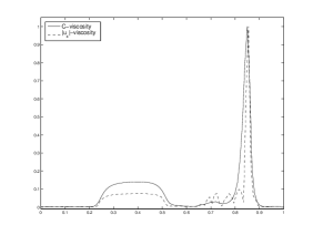
(a) The $C$-equation with $G(u_{x})$

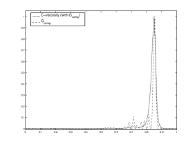
(b) The $C$-equation with $G_{comp}(u_{x})$

Figure 1: A comparison of the artificial viscosity profile produced by the $C$-method and the classical Richtmyer-type approach for the Sod shock tube at $t=.2$. Figures (a) and (b) are with the compression switch off and on, respectively. The smooth solid line is the $C$-method solution, while the oscillatory dashed line is the $|u_{x}|$-Richtmyer-type viscosity.

A useful feature of the $C$-method is the ability to tune parameters in the $C$-equation to generate non-oscillatory behavior. Though we are quite explicit on the form of the $C$-equation in (9b), a simple modification allows for the diffusion coefficient to be problem dependent, i.e. allowing for a choice of positive constant $\gamma>0$ and replacing the diffusion term with

$$-\gamma S({\bf u}^{\epsilon})\partial^{2}_{x}C^{\epsilon}\,.$$

In most of the forthcoming experiments, we fix $\gamma=1$, but we note that choosing larger $\gamma$ can yield smoother solution profiles as the profile of $C$ will be less localized. The parameter $\gamma$ is a time-relaxation parameter, and can be viewed in an analogous fashion to the time-relaxation parameter present in Cahn-Hilliard and Ginzburg-Landau theories. For very slow moving shocks, the time-relaxation can be adjusted to scale with the shock speed.

We find this to be an effective approach for the flattening procedure discussed in [9] for removing oscillations that form to the left of a slowly right-moving shock. Moreover, Roberts [37] concludes that a differentiable form of the numerical flux construction appears necessary to remove downstream long-wavelength oscillations caused by slow shock motion. We use the $C$-method to analyze this.

Using the slow-shock initial conditions outlined in Quirk [12], in Figure 2 we show the success of the FEM-C (outlined below in Section 3.2) in removing these oscillations when choosing $\gamma=1$ (Fig. 2(a)) and $\gamma=100$ (Fig. 2(b)).

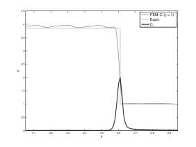
(a) $\gamma=1$

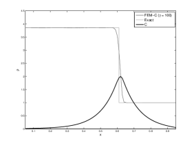
(b) $\gamma=100$

Figure 2: Application of FEM-C to a very slowly moving shock

2.9 Convergence of the $C$-method in the limit of zero mesh size

2.9.1 The isentropic case

We sketch the proof for the isentropic Euler equations given by

$$(\rho u)_{t}+(\rho u^{2}+p)_{x} =0,$$ (20a)

$$\rho_{t}+(\rho u)_{x} =0\,,$$ (20b)

$$p(\rho) =\rho^{\gamma}\,,$$ (20c)

where $\gamma>1$.

To simplify the notation, we set $\tilde{\beta}=1$, and set the momentum $m^{\epsilon}=\rho^{\epsilon}u^{\epsilon}$. Following (9), we write the $C$-method version of (20) as

$$m^{\epsilon}_{t}+[(m^{\epsilon})^{2}/\rho^{\epsilon}+p^{\epsilon}]_{x} =\epsilon^{2}[C^{\epsilon,\delta}m^{\epsilon}_{x}]_{x},$$ (21a)

$$\rho^{\epsilon}_{t}+m^{\epsilon}_{x} =\epsilon^{2}(C^{\epsilon,\delta}\rho_{x})_{x}\,,$$ (21b)

$$p^{\epsilon}(\rho^{\epsilon}) =(\rho^{\epsilon})^{\gamma}\,,$$ (21c)

$$C^{\epsilon}_{t}-S(u^{\epsilon})C^{\epsilon}_{xx}+\frac{S(u^{\epsilon})}{\epsilon}C^{\epsilon} =S(u^{\epsilon})G(u^{\epsilon}_{x})\,,$$ (21d)

or (21a,b) can equivalently in terms of the vector ${\bf u^{\epsilon}}=(m^{\epsilon},\rho^{\epsilon})$ and flux ${\bf f(u^{\epsilon})}=((m^{\epsilon})^{2}/\rho^{\epsilon}+(\rho^{\epsilon})^{\gamma}\ ,\ m^{\epsilon})$ as

$${\bf u^{\epsilon}}_{t}+{\bf f(u^{\epsilon})}_{x}=\epsilon^{2}\left[\mathcal{C}{\bf u^{\epsilon}}_{x}\right]_{x}\,,$$ (21’)

where $\mathcal{C}$ denotes a diagonal 2x2 matrix with entries $C^{\epsilon,\delta}$ which is strictly positive-definite. Recall that $G(u^{\epsilon})=|u^{\epsilon}_{x}|/\max|u^{\epsilon}_{x}|$, satisfies $G\geq 0$, and that $S(u^{\epsilon})=\max(|u^{\epsilon}+c|,|u^{\epsilon}-c|)$, with $c$ denoting the sound speed. On any time interval $[0,T]$, the maximum wave speed $S(u^{\epsilon})$ is uniformly strictly positive; thus, as the initial data for $C^{\epsilon}_{t=0}\geq 0$, the maximum principle shows that $C^{\epsilon}(x,t)$ must be non-negative. We remark that while the use of $C^{\epsilon,\delta}=C^{\epsilon}+\delta$ as the coefficient is not required for the numerics, as $\delta$ is taken much smaller than the mesh size $\Delta x$, strict positivity of $\mathcal{C}$ simplifies the proof of regularity of solutions to (21) as well as the convergence argument.

To avoid issues with spatial boundaries, we shall assume periodic boundary conditions for our spatial domain. Note that in this case, the fundamental theorem of calculus shows that $\frac{d}{dt}\int\rho(x,t)\,dx=0$ and that mass is conserved.

2.9.2 The basic energy law

In order to prove that solutions to (21) converge to solutions of (20), we must establish $\epsilon$-independent estimates for solutions of (21). To do so, we multiply equation (21a) by $u^{\epsilon}$, integrate over our spatial domain, and make use of the equation (21b) to find that any weak solution to (21) must verify the basic energy law

$$\frac{d}{dt}\left[\int{\frac{1}{2}}\rho^{\epsilon}(u^{\epsilon})^{2}\,dx+{\frac{1}{\gamma-1}}\int p^{\epsilon}\,dx\right]\leq-\epsilon^{2}\int C^{\epsilon,\delta}\rho^{\epsilon}\,(u^{\epsilon}_{x})^{2}\,dx-\epsilon^{2}\gamma\int C^{\epsilon,\delta}(\rho^{\epsilon})^{\gamma-2}(\rho^{\epsilon}_{x})^{2}\,dx\,.$$ (22)

(The inequality in (22) is due to the lower semi-continuity of weak convergence and is replaced with equality for solutions which are sufficiently regular.) Thus, the total energy of isentropic gas dynamics is dissipated according to the right-hand side of (22), and for each $\epsilon>0$, we see that $u^{\epsilon}_{x}$ and $\rho^{\epsilon}_{x}$ are square-integrable (in $L^{2}$) for almost every instant of time, if the density $\rho^{\epsilon}\geq\lambda>0$, that is, if $\rho^{\epsilon}$ avoids vacuum. We shall explain below that this is indeed the case.

2.9.3 Regularity of solutions ${\bf u^{\epsilon}}$

The reaction-diffusion equation (21d) is a uniformly parabolic equation. According to the energy law, and as a consequence of Sobolev’s theorem, $u^{\epsilon}$ is a bounded function; furthermore, the right-hand side of (21d) is in $L^{2}$. It is standard, from the regularity theory of uniformly parabolic equations, that $C^{\epsilon}$ then has two spatial (weak) derivatives which are square-integrable. This, in turn, shows that for $\epsilon>0$, solutions ${\bf u^{\epsilon}}$ possess three spatial (weak) derivative which are square-integrable for almost every instant of time. This implies that solutions ${\bf u^{\epsilon}}$ are classically differentiable in both space and time.

Furthermore, by using the symmetrizing matrix $\left[\begin{array}[]{lr}\rho^{\epsilon}&0\\ 0&\gamma(\rho^{\epsilon})^{\gamma-2})\end{array}\right]$ we can show that $(u^{\epsilon}(\cdot,t),\rho^{\epsilon}(\cdot,t))$ are, independently of $\epsilon$ and $t$, uniformly bounded in the Sobolev space $H^{2}$ (consisting of measurable functions with two weak derivatives in $L^{2}$), and thus we may take a pointwise limit of this sequence as $\epsilon\to 0$, in the event that the time-interval is sufficiently small as to ensure that a shock has not yet formed. Of course, we are interested, in convergence to discontinuous profiles, so we address this next.

2.9.4 Convergence to the entropy solution

We shall now provide a sketch of the limit as $\epsilon\to 0$. A function $\eta:\mathbb{R}^{2}\to\mathbb{R}$ is called an entropy for (20) with entropy flux $q:\mathbb{R}^{2}\to\mathbb{R}$ if smooth solutions ${\bf u}$ satisfy the additional conservation law

$$\eta({\bf u})_{t}+q({\bf u})_{x}=0\,.$$ (23)

In non-conservative form, (20) and (23) are written as

$${\bf u}_{t}+\nabla f({\bf u}){\bf u}_{x}=0\,,\ \ \nabla\eta({\bf u}){\bf u}_{t}+\nabla q({\bf u}){\bf u}_{x}=0\,,$$

from which we obtain the compatibility condition between $\eta$ and $q$,

$$\nabla\eta({\bf u})\,\nabla f({\bf u})=\nabla q({\bf u})\,.$$ (24)

The pair $(\eta,q)$ satisfy (23) if and only if condition (24) holds. Moreover, a weak solution to (20) is the unique entropy solution if

$$\eta({\bf u})_{t}+q({\bf u})_{x}\leq 0\,.$$ (25)

For isentropic gas dynamics we can set

$$\eta(m,\rho)=\frac{m^{2}}{2\rho}+\frac{\rho^{\gamma}}{\gamma-1}$$

which is the total energy, with corresponding entropy flux

$$q(m,\rho)=\left[\frac{m^{2}}{2\rho}+\frac{\gamma}{\gamma-1}\rho^{\gamma}\right]\frac{m}{\rho}\,.$$

We observe that $\nabla^{2}\eta(m,\rho)$ is strongly convex as long as $\rho>0$.

For the sequence of solution ${\bf u^{\epsilon}}$ of (21), suppose that as $\epsilon\to 0$, ${\bf u}^{\epsilon}$ converges boundedly (almost everywhere) to a weak solution ${\bf u}$ of (20). We claim that if $(\eta,q)$ satisfy (23), then (25) holds in the distributional sense. To see that this is the case, we take the inner-product of $\nabla\eta({\bf u}^{\epsilon})$ with equation (21’), and find that

$$\eta({\bf u}^{\epsilon})_{t}+q({\bf u}^{\epsilon})_{x} =\epsilon^{2}\nabla\eta({\bf u}^{\epsilon})\left[\mathcal{C}{\bf u}^{\epsilon}_{x}\right]_{x}$$

$$=\epsilon^{2}\left[\mathcal{C}\eta({\bf u}^{\epsilon})_{x}\right]_{x}-\epsilon^{2}[{\bf u}^{\epsilon}_{x}]^{T}\,\mathcal{C}\,\nabla^{2}\eta({\bf u}^{\epsilon}){\bf u}^{\epsilon}_{x}\,.$$

Integrating over the spatial domain and then over the time interval $[0,T]$ yields

$$\int\eta({\bf u}^{\epsilon}(x,T))dx-\int\eta({\bf u}^{\epsilon}(x,0))dx=-\epsilon^{2}\int_{0}^{T}\int[{\bf u}^{\epsilon}_{x}]^{T}\,\mathcal{C}\,\nabla^{2}\eta({\bf u}^{\epsilon}){\bf u}^{\epsilon}_{x}\,dx\,dt\,,$$

from which it follows that

$$\int_{0}^{T}\int|\epsilon{\bf u}^{\epsilon}_{x}|^{2}\,dx\,dt\leq\bar{c}$$ (26)

where the constant $\bar{c}$ depends upon $\delta$, the minimum value of density, and the entropy in the initial data. For a smooth, non-negative test function $\psi$ with compact support in the strip $\mathcal{I}\times(0,T)$,

$$\iint\eta({\bf u}^{\epsilon}\phi_{t}+q({\bf u}^{\epsilon})\phi_{x}\,dxdt=\epsilon\iint\mathcal{C}(\epsilon{\bf u}^{\epsilon})_{x}\phi_{x}\,dxdt+\iint\epsilon^{2}[{\bf u}^{\epsilon}_{x}]^{T}\,\mathcal{C}\,\nabla^{2}\eta({\bf u}^{\epsilon}){\bf u}^{\epsilon}_{x}\phi\,dxdt\,.$$

Thanks to (26), the first term on the right-hand side goes to zero like $\epsilon$, while the second term is non-negative, since $\nabla^{2}\eta({\bf u}^{\epsilon})$ is positive-definite (since $\eta$ is strongly convex) as is $\mathcal{C}$. Thus, as $\epsilon\to 0$, we recover the entropy inequality (25).

It remains to discuss the assumptions concerning the bounded convergence of ${\bf u}^{\epsilon}$ to ${\bf u}$, as well as the uniform bound from below $\rho^{\epsilon}\geq\nu>0$. The argument relies on finding a priori bounds on the amplitudes of solutions to (21). If it is the case that uniformly in $\epsilon>0$,

$$|{\bf u}^{\epsilon}|\leq M\text{ and }0<\nu\leq\rho^{\epsilon}\,,$$

then the compensated-compactness approach for isentropic Euler pioneered by DiPerna [33] and made much more general by Lions, Perthame, & Souganidis [34] provides a subsequence of ${\bf u}^{\epsilon}$ converging pointwise (almost everywhere) to a solution ${\bf u}$ of (20).

For isentropic gas dynamics, our approximation (21) preserves the invariant quadrants of the inviscid dynamics (just as in the case of uniform artificial viscosity) and provides the bound $|{\bf u}^{\epsilon}|\leq M$ as long as $0<\nu\leq\rho^{\epsilon}$ for some $\nu$. In particular, the Riemann invariants $w=u+\frac{2\gamma}{\gamma-1}\rho^{\sqrt{\gamma-1}}$ and $z=u-\frac{2\gamma}{\gamma-1}\rho^{\sqrt{\gamma-1}}$ satisfy $w(x,t)\leq\sup w|_{t=0}$ and $-z(x,t)\leq\sup(-z_{t=0})$ and the intersection of these half-planes provides the invariant quadrant (see Chueh, Conley, & Smoller [38]), and hence the desired bound $|{\bf u}^{\epsilon}|\leq M$ as long as vacuum is avoided.

Finally, the fact that we have the lower-bound $0<\nu\leq\rho^{\epsilon}$ is an immediate consequence of the strong maximum principle.

2.10 The $C$-equation as a gradient flow

Notice that equilibrium solutions to the $C$-equation are minimizers of the following functional (we drop the superscript $\epsilon$):

$$\mathcal{E}_{G}(C)=\int\left({\frac{1}{2}}C_{x}^{2}-G(u_{x})C+{\frac{1}{2\epsilon}}C^{2}\right)\,dx\,.$$

In the absence of a forcing function $G(u_{x})$, this reduces to

$$\mathcal{E}_{0}(C)={\frac{1}{2}}\int\left({C_{x}^{2}}+{\frac{1}{\epsilon}}C^{2}\right)\,dx\,.$$ (27)

The first term is commonly referred to as the Dirichlet energy and its minimizers are harmonic functions. The second term can be viewed as a penalization of the Dirichlet energy. In particular, because the energy functional is bounded by a constant independent of $\epsilon>0$, the penalization term constrains $C$ to be $O(\sqrt{\epsilon})$. Thus, minimizers are trying to be harmonic while minimizing their support.

The $C$-equation can be written as a classical gradient flow equation

$$\frac{dC}{dt}=-S(u)\nabla\mathcal{E}_{G}(C)\,,$$

where the gradient is computed relative to the $L^{2}$ inner-product. Thus the heat operator in the $C$-equation, $\partial_{t}-\partial^{2}_{x}$, smooths the forcing in space-time, while the reaction term $S(u)/\epsilon C$ minimizes the support of the smoothed profile. This is very much related to the theories of Cahn-Hilliard and Ginzburg-Landau gradient flows, and we intend to examine this connection in subsequent papers.

3 Numerical Schemes

We describe two very different numerical algorithms in the context of our $C$-method. First, we outline a classical continuous finite-element discretization, yielding FEM-C and FEM-$|u_{x}|$ (based on classical artificial viscosity). Second, we discuss a simple WENO-based scheme for compressible Euler that upwinds solely based on the sign of the velocity $u$. To this scheme, we apply a slightly modified $C$-method resulting in our WENO-C algorithm.

For the purpose of comparison, we also implement two additional numerical methods. The first is a second-order central-differencing scheme of Nessayhu-Tadmor (NT), a nice and simple method which serves as a base-line for our FEM-C comparisons. The second scheme is a very competitive WENO scheme that utilizes a Godunov-based upwinding based upon characteristic decompositions (WENO-G). This will serve as a benchmark for our WENO-C scheme.

3.1 Notation for discrete solutions

To compute approximations to (4), we subdivide space-time into a collection of spatial nodes $\{x_{i}\}$ and temporal nodes $\{t_{n}\}$. We denote the computed approximate solution by

$${\bf u}^{n}_{i}\approx{\bf u}(x_{i},t_{n}),$$

noting that for fixed $i$ and $n$, ${\bf u}^{n}_{i}$ is a 3-vector of solution components, i.e.,

$${\bf u}^{n}_{i}=\left[\begin{array}[]{c}\rho^{n}_{i}\\ m^{n}_{i}\\ E^{n}_{i}\end{array}\right].$$

It is important to note that we use the notation ${\bf u}^{n}_{i}$ for both pointwise approximations to ${\bf u}$, (acquired via FEM-C) and approximations to the cell-average values of ${\bf u}$ (acquired via WENO-C).

A subscripted quantity $w_{i}$ denotes the vector itself and the individual components of the vector. We overload this notation so to not cause any confusion between functions defined over a continuum versus those defined only at a finite number of points.

In FEM-C and WENO-C, we discretize (9) (or some slight modification) with $\epsilon=\Delta x$, and use the above notation for the computed solution. We also denote the approximation to $C$ by $C^{n}_{i}$.

3.2 FEM-C and FEM-$|u_{x}|$: A Second-Order Continuous-Galerkin Finite-Element Scheme

We choose a second-order continuous-Galerkin finite-element scheme to provide a discretization of (9), subsequently defining our FEM-C scheme.

We subdivide $\mathcal{I}$ with $N+1$ (for $N$ even)-uniformly spaced nodes $\{x_{i}\}$ separated by a distance $\Delta x$. In the FEM community, spatial discretization size is more commonly referred by element-width; to maintain consistency with the literature, we refer to the inter-nodal regions as cells. Since we use a continuous FEM, the degrees-of-freedom are defined at the cell-edges (as opposed to cell-centers).

For use in our FEM implementation, it is useful to consider the variational form of (9). At the continuum level, $({\bf u}^{\epsilon},C^{\epsilon})$ satisfy

$$\int_{\mathcal{I}}\left[\partial_{t}{\bf u}^{\epsilon}\cdot\Phi-{\bf F}({\bf u}^{\epsilon})\cdot\partial_{x}\Phi+\beta\epsilon^{2}{\frac{\underset{\mathcal{I}}{\max}\ |\partial_{x}u^{\epsilon}|}{\underset{\mathcal{I}}{\max}\ C^{\epsilon}}}C^{\epsilon}\partial_{x}{\bf u}^{\epsilon}\cdot\partial_{x}\Phi\right]\,dx=0\,,$$ (28a)

$$\int_{\mathcal{I}}\left[\partial_{t}C^{\epsilon}\phi+S({\bf u^{\epsilon}})\left(\epsilon\partial_{x}C^{\epsilon}\partial_{x}\phi+\frac{1}{\epsilon}C^{\epsilon}\phi\right)\right]\,dx=\int_{\mathcal{I}}S({\bf u}^{\epsilon})G(\partial_{x}u^{\epsilon})\phi\ dx$$ (28b)

for almost every $t$, for all vector-valued test functions $\Phi$, and all scalar-valued test functions $\phi$.

Using the finite-element spatial discretization based on piecewise second-order Lagrange polynomials, we construct operators $\mathcal{A}_{\text{FEM}}$ and $\mathcal{B}_{\text{FEM}}$, corresponding to the non-time-differentiated terms in (28a) and (28b), respectively. Using these discrete operators, we write the semi-discrete form of (28a) and (28b) as

$$\partial_{t}\left[\begin{array}[]{c}{\bf u}_{i}\\ C_{i}\end{array}\right]+\left[\begin{array}[]{c}\mathcal{A}_{\text{FEM}}({\bf u}_{i},C_{i})\\ \mathcal{B}_{\text{FEM}}({\bf u}_{i},C_{i})\end{array}\right]=0$$ (29)

where ${\bf u}_{i}$ and $C_{i}$ represent the nodal values of an approximation to ${\bf u}^{\epsilon}$ and $C^{\epsilon}$ for which $\epsilon=\Delta x$ (see Section 2.6). For a standard reference on the details of this procedure, see Larsson & Thomée [39].

The time-differentiation in (29) is approximated by a diagonally-implict second-order time-stepping procedure; first we predict ${\bf u}_{i}^{n+1}$ to and solve the implicit set of equations for $C_{i}^{n+1}$ and follow by implicitly solving for ${\bf u}_{i}^{n+1}$ using $C_{i}^{n+1}$. Our fully discrete scheme is given by

$${\bf\tilde{u}}_{i}^{n+1} ={\bf u}_{i}^{n}+\mathcal{A}_{FEM}({\bf u}_{i}^{n},C_{i}^{n}),$$ (30a)

$$C_{i}^{n+1} =C_{i}^{n}+\frac{t_{n+1}-t_{n}}{2}\left[\mathcal{B}_{FEM}({\bf\tilde{u}}_{i}^{n+1},C_{i}^{n+1})+\mathcal{B}_{FEM}({\bf u}_{i}^{n},C_{i}^{n})\right],$$ (30b)

$${\bf u}_{i}^{n+1} ={\bf u}_{i}^{n}+\frac{t_{n+1}-t_{n}}{2}\left[\mathcal{A}_{FEM}({\bf u}_{i}^{n+1},C_{i}^{n+1})+\mathcal{A}_{FEM}({\bf u}_{i}^{n},C_{i}^{n})\right].$$ (30c)

For smooth solutions, where artificial viscosity is not necessary, our FEM-C scheme is second-order accurate in both space and time when the error is measured in the $L^{1}$-norm. Moreover, the addition the artificial viscosity obtained through the $C$-method is formally a second-order perturbation (in $\Delta x$) and we have verified this accuracy when $\beta>0$ (again, for smooth ${\bf u}_{0}$). For ${\bf u}_{0}$ containing jump discontinuities, the given scheme is no longer second-order accurate on all of $\mathcal{I}$ but preserves second-order accuracy in the smooth regions away from discontinuities.

For the classical artificial viscosity schemes (8), the C-equation is no longer used but we require a similar step to predict the velocity for use in the diffusion coefficient. This analogous scheme, is referred to as the FEM-$|u_{x}|$ scheme.

3.3 WENO-C: A Simple WENO scheme using the $C$-method

Our WENO-based scheme is motivated by Leonard’s finite volume schemes ([40], pg. 65). Upwinding is performed solely based on the sign of the velocity at cell-edges, and the WENO reconstruction procedure is formally fifth-order.

We divide the interval $\mathcal{I}$ into $N$ equally sized cells of width $\Delta x$, identifying the $N$ degrees-of-freedom as cell-averages over cells centered at the $x_{i}$. The cell edges are denoted using the fraction index, i.e.

$$x_{i+1/2}=\frac{x_{i}+x_{i+1}}{2}$$

Subsequently, we denote a cell-averaged quantity by $w_{i}$ and its values at the left and right endpoints by $w_{i-1/2}$ and $w_{i+1/2}$, respectively.

Given a vector $w_{i}$, corresponding to cell-average values, and vectors $z_{i-1/2}$, $z_{i+1/2}$ corresponding to left and right cell-edge values, we define the $j$th component of vector

$$\left[\text{WENO}(w_{i},z_{i\pm 1/2})\right]_{j}=\frac{1}{\Delta x}\left(\tilde{w}_{j+1/2}z_{j+1/2}-\tilde{w}_{j-1/2}z_{j-1/2}\right)$$

where the cell-edge values of $\tilde{w}_{j+1/2}$ are calculated using a fifth-order WENO reconstruction, upwinding based upon the sign of $z_{j+1/2}$.

For the flux in the energy equation, we use

$$\left[\text{WENO}_{E}(E_{i},u_{i\pm 1/2})\right]_{j}=\frac{1}{\Delta x}\Big{(}\tilde{E}_{j+1/2}u_{j+1/2}\frac{(1+\frac{p_{j}}{E_{j}})+(1+\frac{p_{j+1}}{E_{j+1}})}{2}-\\ \tilde{E}_{j-1/2}u_{j-1/2}\frac{(1+\frac{p_{j-1}}{E_{j-1}})+(1+\frac{p_{j}}{E_{j}})}{2}\Big{)}.$$ (31)

Using this simplified WENO-based reconstruction, we construct the operators $\mathcal{A}_{\text{WENO}}$ and $\mathcal{B}_{\text{WENO}}$ where

$$\left[\mathcal{A}_{\text{WENO}}\left(\left[\begin{array}[]{c}\rho_{i}\\ m_{i}\\ E_{i}\end{array}\right],\ C_{i}\right)\right]=\left[\begin{array}[]{c}\text{WENO}(\rho_{i},u_{i\pm 1/2})\\ \text{WENO}(m_{i},u_{i\pm 1/2})+\tilde{\partial}p_{i}-{\frac{\tilde{\partial}_{C}u_{i+1/2}-\tilde{\partial}_{C}u_{i-1/2}}{\Delta x}}\\ \text{WENO}_{E}(E_{i},u_{i\pm 1/2})\end{array}\right]$$ (32a)

$$\mathcal{B}_{\text{WENO}}\left(\left[\begin{array}[]{c}\rho_{i}\\ m_{i}\\ E_{i}\end{array}\right],\ C_{i}\right)=-\frac{S({\bf u}_{i})}{\Delta x}\left[C_{i}-G(\tilde{\partial}u_{i})\right]+\frac{\tilde{\partial}_{S}C_{i+1/2}-\tilde{\partial}_{S}C_{i-1/2}}{\Delta x}.$$ (32b)

where for a general quantity $w_{i}$, defined at the cell-centers, we denote

$$w_{i+1/2}=\frac{w_{i+1}+w_{i}}{2},\quad\tilde{\partial}w_{i}:=\frac{w_{i+1}-w_{i-1}}{2\Delta x},\quad\tilde{\partial}w_{i+1/2}=\frac{w_{i+1}-w_{i}}{\Delta x}.$$

We also use the shorthand notation

$$\tilde{\partial}_{C}u_{i+1/2}=\beta\ \Delta x^{2}\ \max_{i}\left|\tilde{\partial}u_{i+1/2}\right|\ \frac{C_{i+1/2}}{\underset{i}{\max}\ C_{i}}\ \rho_{i+1/2}\ \tilde{\partial}u_{i+1/2},$$

and

$$\tilde{\partial}_{S}C=\Delta x\ S({\bf u}_{i})\ \tilde{\partial}C_{i+1/2}.$$

Using the above definitions, we define the semi-discrete form

$$\partial_{t}\left[\begin{array}[]{c}{\bf u}_{i}\\ C_{i}\end{array}\right]+\frac{1}{\Delta x}\left[\begin{array}[]{c}\mathcal{A}_{\text{WENO}}({\bf u}_{i},C_{i})\\ \mathcal{B}_{\text{WENO}}({\bf u}_{i},C_{i})\end{array}\right]=0$$ (33)

and we generate the sequence of iterates ${\bf u}^{n}_{i}$ and $C^{n}_{i}$ with a standard fourth-order Runge-Kutta time-stepper.

The resulting discretization outlined above is a slight variation on that outlined in (9). While the amount of artificial viscosity $C(x,t)$ is controlled by only the velocity, we only add artificial viscosity to the momentum equation. This change is based upon the fact that WENO already minimizes the production of numerical oscillations and the addition of artificial viscosity is primarily intended on stabilizing the solution near strong shocks, whereas standalone WENO may lose stability. Without dissipation on the right-hand side of the mass equation, it is necessary to modify the artificial viscosity on the momentum equation as follows:

$$\epsilon^{2}\tilde{\beta}\partial_{x}(C\partial_{x}(\rho u))\to\epsilon^{2}\tilde{\beta}\partial_{x}(C\rho\partial_{x}u)\,.$$ (34)

This modification allows the $C$-method to maintain a basic energy law (in fact, it is the energy law (22) with the last term on the right-hand side), and simultaneously permits higher accuracy for our WENO-based scheme.

3.4 NT: A Second-order Central-Differencing scheme of Nessayhu-Tadmor

The central-differencing scheme of Nessyahu and Tadmor is an extension of the first-order Lax-Fredrichs finite difference scheme in which linear, MUSCL-based reconstructions are used to yield a second-order accurate scheme. The resulting scheme is extremely easy to implement (a FORTRAN code for 2-D problems is given in the Appendix of [16]) and does not require the use of Riemann solvers or characteristic directions for the purpose of upwinding. The NT scheme allows for various choices of limiters to enforce TVD or ENO but the UNO-limiter (see Harten & Osher [41]) is the most successful for our range of experiments.

Though that NT is easy to implement and is easy generalized to multi-D (yielding the JT-scheme [16]), it merely serves as a base-line comparison for our FEM-C. Both FEM-C and NT are second-order, but FEM-C turns out to be far less diffusive by comparison.

3.5 WENO-G: WENO with Godunov-based upwinding

In [31] the authors study a fifth-order, WENO-based discretization, upwinding by virtue of a high-accuracy Godunov-scheme. Their scheme has the usual trait of WENO, offering minimal diffusion near extrema, and has the added stabilization and accuracy of higher-order Godunov solvers. For a more in-depth description, see [31].

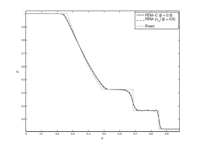
(a) Complete density profile

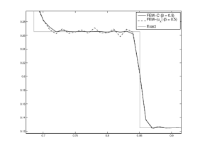
(b) Zoom-in at shock

Figure 3: Comparison of FEM-C and FEM-$|u_{x}|$, for the Sod shock-tube experiment with $N=100$, $T=0.2$. $\beta=0.5$ for both FEM-C and FEM-$|u_{x}|$.

4 Sod shock-tube problem

For the classic Sod shock-tube problem, we consider the domain $\mathcal{I}=[0,1]$ along with the initial conditions

$$\left(\begin{array}[]{c}\rho_{0}(x)\\ m_{0}(x)\\ E_{0}(x)\end{array}\right)=\left(\begin{array}[]{c}1\\ 0\\ 2.5\end{array}\right){\bf 1}_{[0,\frac{1}{2})}(x)+\left(\begin{array}[]{c}0.125\\ 0\\ 0.25\end{array}\right){\bf 1}_{[\frac{1}{2},1]}(x),$$ (35)

imposing natural boundary conditions at $x=0$ and $x=1$. This standard test problem, first considered in Sod [42], is a preliminary test for the viability of numerical schemes. An exact solution is known for this problem and consists of two nonlinear waves (one shock and one rarefaction) along with a contact discontinuity.

In Figure 3(b) we compare the results of FEM-C and FEM-$|u_{x}|$ at $t=0.2$ using $N=100$ cells. We note that this comparison uses the standard choice of $G$ in (9) since we are merely concerned with the C-equation performing as a smooth version of classical artificial viscosity schemes. Unlike comparisons with the schemes based on cell-averages, we compare the nodal values of FEM-C and FEM-$|u_{x}|$. In this comparison, we choose $\beta=0.5$ for both schemes and see that the accuracy of both FEM-C and FEM-$|u_{x}|$ are quite comparable and each scheme resolves the shock in 3 cells. However, we notice noise in FEM-$|u_{x}|$ near the shock. In Figure 3(b) this observation is exemplified and we see that FEM-C is relatively non-oscillatory by comparison.

To limit these oscillations generated by FEM-$|u_{x}|$, we increase $\beta$ by a factor of $6$ and compare the resulting density in Figure 4. In Figure 4(b) we can see a significant loss in accuracy when increasing to $\beta=3$. Furthermore, in Figure 4(a) we see FEM-$|u_{x}|$ requires 6 cells to capture the shock.

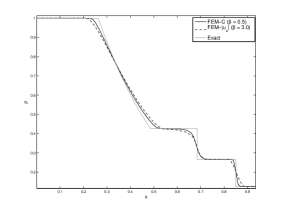
(a) Complete density profile

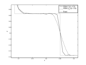
(b) Zoom-in at shock

Figure 4: Comparison of FEM-C and FEM-$|u_{x}|$, for the Sod shock-tube experiment with $N=100$, $T=0.2$. $\beta=0.5$ for FEM-C and $\beta=3.0$ for FEM-$|u_{x}|$.

In Figure 5 we compare the results of the FEM-C scheme versus NT and WENO-G. Each simulation is performed with $N=100$ and for the FEM-C scheme we choose $\beta=0.4$ and now use $G_{comp}$ (see Section 2.5).

Each scheme produces similar resolution of the shock and contact discontinuity, capturing the shock in $3$ cells and the contact discontinuity in $6$ cells. The NT-scheme produces small, smooth, non-physical oscillations as the density transitions from the rarefaction to the lower states, and performs the worst at the rarefaction. Both FEM-C and WENO-G are essentially non-oscillatory and despite WENO-C performing slightly better at the rarefaction, the results are virtually indistinguishable at the shock and contact discontinuity.

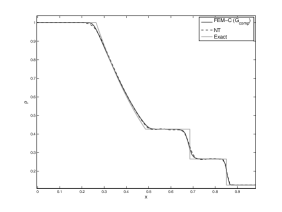
(a) FEM-C vs. NT

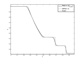
(b) FEM-C vs. WENO

Figure 5: Comparisons of FEM-C against NT and WENO schemes, for the Sod shock-tube experiment with $N=100$ and $T=0.2$.

5 Osher-Shu shock-tube problem

For the problem of Osher-Shu, we consider the domain $\mathcal{I}=[-1,1]$ along with initial conditions

$$\left(\begin{array}[]{c}\rho_{0}(x)\\ m_{0}(x)\\ E_{0}(x)\end{array}\right)=\left(\begin{array}[]{c}3.857143\\ 10.14185\\ 39.1666\end{array}\right){\bf 1}_{[-1,-0.8)}(x)+\left(\begin{array}[]{c}1+0.2\sin(5\pi x)\\ 0\\ 2.5\end{array}\right){\bf 1}_{[-0.8,1]}(x),$$ (36)

imposing natural boundary conditions at $x=-1$ and $x=1$

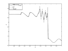
(a) FEM-C vs. NT

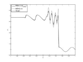
(b) FEM-C vs. WENO

Figure 6: Comparisons of FEM-C against NT and WENO schemes, for the Osher-Shu shock-tube experiment with $N=200$ and $T=0.36$.

This moderately difficult test problem, first considered in [3], proves to be more difficult for numerical schemes due to the evolution a shock-wave which interacts with an entropy-wave; care is required to accurately capture the amplitudes of the post-shock entropy waves. Since the density is not monotone, standard flux limiters may unnecessarily apply too much dissipation at local-extrema, significantly reducing accuracy. An exact solution for this problem is not available and our ‘Exact’ solution in our plots is generated using the DG-solver furnished in Hesthaven & Warburton [43] with 3200 cells.

In Figure 6 we compare the results of FEM-C (we choose $\beta=0.5$ and use $G_{comp}$), versus NT and WENO-G at $t=0.36$. In Figure 6(a) we see that NT diffuses the post-shock amplitudes and FEM-C provides far superior results. On the other hand, in Figure 6(b) we see that all but one of the post-shock amplitudes are slightly better for the WENO-G scheme. This insufficiency of the FEM-C scheme is not completely surprising as the FEM-C is only formally second-order versus the fifth-order accuracy of the WENO-G scheme.

Noting this insufficiency of the FEM-C scheme, we compare the WENO-G scheme with WENO-C in Figure 7(a) and see the WENO-C scheme is more accurate in resolving the post-shock amplitudes. This comes at a price however, as we see WENO-G is more accurate in the N-wave region $[-0.6,0]$.

Furthermore, it is interesting to note that in Figure 7(b) where we choose $\beta=0$ in our simplified WENO-scheme, we see that the C-equation is not necessary for Osher-Shu. As we see in Section 6 this ceases to be the case as the collision of strong shock waves require stabilization.

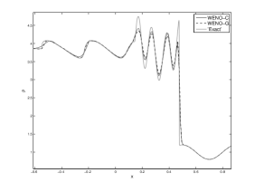
(a) WENO-C vs. WENO-G

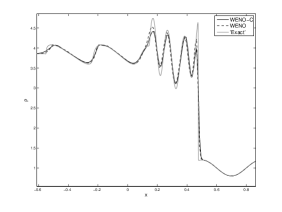
(b) WENO-C vs. WENO

Figure 7: Comparisons of WENO-C with WENO-G and our WENO scheme with artificial viscosity deactivated, for the Osher-Shu shock-tube experiment with $N=200$ and $T=0.36$.

6 Woodward-Colella Blast Wave

The colliding blast wave problem of Woodward-Collella is posed on the domain $\mathcal{I}=[0,1]$ with initial conditions

$$\rho_{0}(x)=1,$$

$$m_{0}(x)=0,$$

$$E_{0}(x)=250\cdot{\bf 1}_{[0.9,1]}+0.25\cdot{\bf 1}_{[0.1,0.9)}+2500\cdot{\bf 1}_{[0,0.1)},$$

and reflective boundary conditions at $x=0$ and $x=1$. This challenging blast wave problem, considered in [13] tests the ability of a numerical scheme to handle collisions between strong shock waves. Any viable scheme generally requires stabilization at these collisions. For the results of a wide range of schemes applied to this problem, see [9]. An exact solution for this problem is not available and the ‘Exact’ solution in our plots is generated with a 400-cell PPM solver.

As is standard in our sequence of experiments, we provide a comparison of FEM-C ($\beta=0.5$) with NT and WENO-G in Figure 8 at $t=0.038$. It is interesting to note, the use of $G_{comp}$ is far too oscillatory in this difficult test problem; we revert to the standard choice of $G$. We again see that while FEM-C is superior to NT in capturing the amplitude of the two peaks in the density, FEM-C is far too diffusive in comparison to WENO-G.

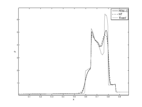
(a) FEM-C vs. NT

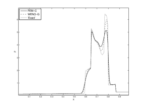
(b) FEM-C vs. WENO

Figure 8: Comparisons of FEM-C against NT and WENO schemes, for the Woodward-Colella blast-tube experiment with $N=400$ and $T=0.038$.

Despite the relative inefficiency of FEM-C compared to WENO-G, it is interesting to note that our FEM-C results (with $N=1200$) are better than the artificial viscosity schemes use in Colella & Woodward [9]. Our scheme is slightly sharper at the shocks and contact discontinuities and is just as accurate in the height of the two peaks.

Before moving to a comparison of WENO-G and WENO-C, in Figure 9(a) we see that our simplified WENO scheme is highly oscillatory due to the strong shock collision, necessitating the use of stabilization. This requirement contrasts to the observations made in Section 5. However, in Figure 9(b), we see that the use of a classical artificial viscosity significantly dampens the instability but moderate oscillations occur and the $C$-method provides similar dampening in a smooth way.

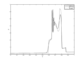
(a) WENO (without stabilization)

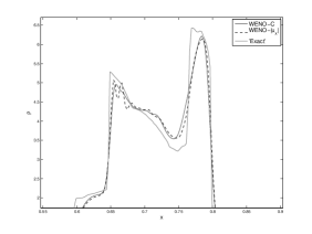
(b) WENO (with stabilization)

Figure 9: WENO with and without stabilization applied to the Woodward-Colella blast-tube experiment with $N=400$ and $T=0.038$.

Finally, in Figure 10 we demonstrate the relative success of WENO-C versus WENO-G. At the left peak, WENO-G is more accurate, but at the right peak the reverse situation occurs. Each scheme provides very good results, and it is clear that WENO-C is a simple alternative to WENO-G which produces similar results for complicated shock interaction.

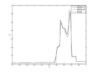
Figure 10: Comparison of WENO-C against WENO-G, for the Woodward-Colella blast-tube experiment with $N=400$ and $T=0.038$.

7 Leblanc shock-tube problem

We conclude our experiments with the Leblanc shock-tube, posed on the domain $\mathcal{I}=[0,9]$, with initial conditions

$$\left(\begin{array}[]{c}\rho_{0}(x)\\ m_{0}(x)\\ E_{0}(x)\end{array}\right)=\left(\begin{array}[]{c}1\\ 0\\ 10^{-1}\end{array}\right){\bf 1}_{[0,3)}(x)+\left(\begin{array}[]{c}10^{-3}\\ 0\\ 10^{-9}\end{array}\right){\bf 1}_{[3,9]}(x)\,,$$ (37)

with natural boundary conditions at $x=0$ and $x=9$, and with the adiabatic constant $\gamma=\frac{5}{3}$.

Because the initial energy $E_{0}$ jumps ten orders of magnitude, a very strong shock wave is produced, making the Leblanc problem an extraordinarily difficult numerical experiment. First , numerical methods tend to over-estimate the correct shock speed whenever the shock wave in the pressure field is not sharply resolved. Second, numerical approximations tend to produce large overshoots in the internal energy

$$e=\frac{p}{(\gamma-1)\rho}$$

at the contact discontinuity. We refer the reader to Liu, Cheng, & Shu [44] and Loubére & Shashkov [45] for a discussion of the difficulties in the numerical simulation of the Leblanc problem for a variety of numerical schemes. The second-order finite-element basis that we use for our FEM-C algorithm is not sufficiently high-order to accurately capture wave speeds in Leblanc, but our fifth-order WENO-C scheme is ideally suited for this difficult test case. We shall present two differing strategies for WENO-C, which both capture the correct shock speed and remove overshoots of the internal energy.

7.1 Strategy One: A $C$ equation for the energy density

As we introduced the $C$-method in equation (9), artificial viscosity is present on the right-hand side of all three conservation laws for momentum, mass, and energy. For the WENO-C algorithm, only viscosity in the momentum equation has been used for the Sod, Osher-Shu, and Woodward-Colella test cases. Due to the strength of the shock in Leblanc, we now return to using artificial viscosity for the energy equation. In our first strategy for this problem, we solve for one additional linear reaction-difffusion equation for a new $C$-coefficient to use on the right-hand side of the energy conservation law.

Specifically, to combat the large overshoot in the internal energy $e$, we solve a second $C$-equation for the coefficient which we label $C_{E}$; the forcing term for the $C_{E}$ equation uses $|\partial_{x}(E/\rho)|/\max|\partial_{x}(E/\rho)|$, replacing $|\partial_{x}u|/\max|\partial_{x}u|$ which forces the $C$-equation for the coefficient $C_{u}$, used for the right-hand side of the momentum equation. In particular, since $C_{u}$ is found using the $G_{comp}$ forcing, activated only in compressive regions when $u_{x}<0$, for the $C_{E}$ equation, we activate the right-hand side only in expansive regions when $u_{x}\geq 0$. To be precise, this modified WENO-C scheme replaces the semi-discrete form (33) with

$$\partial_{t}\left[\begin{array}[]{c}{\bf u}_{i}\\ {\bf C}_{i}\end{array}\right]+\frac{1}{\Delta x}\left[\begin{array}[]{c}\mathcal{\tilde{A}}_{\text{WENO}}({\bf u}_{i},{\bf C}_{i})\\ \mathcal{\tilde{B}}_{\text{WENO}}({\bf u}_{i},{\bf C}_{i})\end{array}\right]=0.$$ (38)

The resulting fully-discrete scheme solves for ${\bf u}^{n}_{i}$ and

$${\bf C}^{n}_{i}=\left(\begin{array}[]{c}C^{n}_{u_{i}}\\ C^{n}_{E_{i}}\end{array}\right)$$

where the modified fluxes $\mathcal{\tilde{A}}_{\text{WENO}}$ and $\mathcal{\tilde{B}}_{\text{WENO}}$ are given by:

$$\left[\mathcal{\tilde{A}}_{\text{WENO}}\left(\left[\begin{array}[]{c}\rho_{i}\\ m_{i}\\ E_{i}\end{array}\right],\left[\begin{array}[]{c}C_{u_{i}}\\ C_{E_{i}}\end{array}\right]\right)\right]=\\ \left[\begin{array}[]{c}\text{WENO}(\rho_{i},u_{i\pm 1/2})\\ \text{WENO}(m_{i},u_{i\pm 1/2})+\tilde{\partial}p_{i}-{\frac{\tilde{\partial}_{C_{u}}u_{i+1/2}-\tilde{\partial}_{C_{u}}u_{i-1/2}}{\Delta x}}\\ \text{WENO}_{E}(E_{i},u_{i\pm 1/2})-{\frac{\tilde{\partial}_{C_{E}}E_{i+1/2}-\tilde{\partial}_{C_{E}}E_{i-1/2}}{\Delta x}}\end{array}\right]$$ (39a)

$$\left[\mathcal{\tilde{B}}_{\text{WENO}}\left(\left[\begin{array}[]{c}\rho_{i}\\ m_{i}\\ E_{i}\end{array}\right],\left[\begin{array}[]{c}C_{u_{i}}\\ C_{E_{i}}\end{array}\right]\right)\right]=\\ \frac{1}{\Delta x}\left[\begin{array}[]{c}-{S({\bf u}_{i})}\left[C_{u_{i}}-G_{comp}(\tilde{\partial}u_{i})\right]+{\tilde{\partial}_{S}C_{u_{i+1/2}}+\tilde{\partial}_{S}C_{u_{i-1/2}}}\\ -{S({\bf u}_{i})}\left[C_{E_{i}}-G_{expand}(\tilde{\partial}(E/\rho)_{i},\tilde{\partial}u_{i})\right]+{\tilde{\partial}_{S}C_{E_{i+1/2}}-\tilde{\partial}_{S}C_{E_{i-1/2}}}.\end{array}\right]$$ (39b)

The expansive-region forcing for $C_{E}$ is given by

$$G_{expand}\left(\tilde{\partial}E_{i},\tilde{\partial}u_{i}\right)=\frac{|\tilde{\partial}(E/\rho)_{i}|}{\underset{i}{\max}|\tilde{\partial}(E/\rho)_{i}|}{\bf 1}_{[0,\infty)}(\tilde{\partial}u_{i})$$ (40)

and we use the shorthand

$$\tilde{\partial}_{C_{u}}u_{i+1/2}=\beta_{u}\ \Delta x^{2}\ \max_{i}\left|\tilde{\partial}u_{i+1/2}\right|\ \frac{C_{u_{i+1/2}}}{\underset{i}{\max}\ C_{u_{i}}}\ \rho_{i+1/2}\ \tilde{\partial}u_{i+1/2},$$

and

$$\tilde{\partial}_{C_{E}}E_{i+1/2}=\beta_{E}\ \Delta x^{2}\ \max_{i}\left|\tilde{\partial}u_{i+1/2}\right|\ \frac{C_{E_{i+1/2}}}{\underset{i}{\max}\ C_{E_{i}}}\rho_{i+1/2}\ \tilde{\partial}(E/\rho)_{i+1/2}.$$

In Figure 11(a) we plot the difference between WENO-C with and without the use of this new equation for $C_{E}$. For WENO-C with $C_{E}$ activated, we choose $\beta_{u}=1.0$ and $\beta_{E}=0.15$; with the $C_{E}$-equation deactivated, we use $\beta_{u}=1.0$ and $\beta_{E}=0$. Observe that activating the $C_{E}$-equation removes the large overshoot at the contact discontinuity. Furthermore, examining the location of the shock, we see that the use of the $C_{E}$-equation produces more accurate approximations of the shock speed.

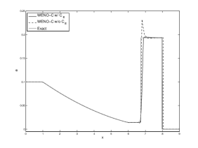
(a) With and without $C_{E}$, $N=1440$

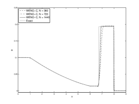
(b) Successive refinements, $N=360,720,1440$

Figure 11: Internal energy plots for WENO-C for the Leblanc shock-tube experiment at $T=6$.

In Figure 11(b) we show the results of WENO-C at $N=360,720,1440$. In this plot, we see very little overshoot at each level of refinement and this small overshoot does not grow with refinement.

7.2 Strategy Two: a new type of viscosity for the energy density

Our second strategy for the Leblanc problem may be viewed as being motivated by the energy dissipation rate of real fluids, and adheres to our framework of only solving one $C$-equation, forced by the normalized modulus of the gradient of velocity. The idea is easy to explain, and we begin by writing the equations for momentum and mass (we drop the superscript $\epsilon$):

$$(\rho u)_{t}+(\rho u^{2}+p)_{x} =\epsilon^{2}\tilde{\beta}(C\rho u_{x})_{x}\,,$$ (41a)

$$\rho_{t}+(\rho u)_{x} =0\,$$ (41b)

$$p =(\gamma-1)\rho\,e\,,$$ (41c)

$$C_{t}-S(u)C_{xx}+\frac{S(u)}{\epsilon}C =S(u)G(u_{x})\,.$$ (41d)

By multiplying the momentum equation by the velocity $u$, integrating over the spatial domain, and using the conservation of mass equation, we find the basic energy law:

$$\frac{d}{dt}\left[\int{\frac{1}{2}}\rho u^{2}\,dx+{\frac{1}{\gamma-1}}\int p\,dx\right]=-\epsilon^{2}\tilde{\beta}\int C\rho\,u_{x}^{2}\,dx\,.$$ (42)

Note, that when $\epsilon=0$, the variable $E$ is exactly the energy density; that is, when $\epsilon=0$, $E={\frac{1}{2}}\rho u^{2}+{\frac{p}{\gamma-1}}$. Thus, we formulate a right-hand side term for the energy equation to ensure the $E$ continues to represent the energy density for $\epsilon>0$. To do, we choose a right-hand side which will provide the same energy law as (42). We introduce the following equation:

$$E_{t}+(uE+up)_{x}=-\epsilon^{2}\tilde{\beta}C\rho\,u_{x}^{2}\,.$$ (43)

The fundamental theorem of calculus shows that integration of (43) provides the same basic energy law as (42). Hence, our second strategy employs the equation (41) together with (43). The interesting feature of the new right-hand side of the energy equation is its nonlinear structure, quadratic in velocity gradients. This energy loss compensates for entropy production, and can become anti-diffusive near contact discontinuities. As such, we shall discretize this set of equations using the very stable Lax-Friedrichs flux. We remark that the term $\epsilon^{2}\tilde{\beta}C\rho\,u_{x}^{2}$ is analogous to the viscous dissipation term of the Navier-Stokes-Fourier system and can be found as a truncation error in [22].

As we noted above, to the best of our knowledge, the most commonly used numerical schemes applied to Leblanc tend to exhibit a significant overshoot in the internal energy $e$ at the contact discontinuity. Furthermore, on coarse meshes ($<2000$ cells), the speed of the shock tends to be inaccurate. Indeed, this is the case for arguably the most widely used WENO implementation, designated WENO-LF-5-RK-4 by Jiang & Shu [5]. This scheme, which we call WENO-LF, uses a Lax-Friedrichs flux-splitting with a $5$th-order WENO reconstruction in space and $4$th-order Runge-Kutta in time.

If we examine the contact discontinuity at $x\approx 6.8$ in Figure 12(a), at resolutions $N=360,720,1440$ we see that WENO-LF exhibits relative overshoots of $12.8\%$, $11.8\%$ and $11.4\%$ respectively. This slow decay of the overshoot suggests that WENO-LF suffers from the Gibbs-phenomenon, despite it’s attempt to quell oscillatory behavior. Examining the shock at $x\approx 8$ we see that the computed shock speeds are inaccurate.

To address the loss of accuracy exhibited by WENO-LF, we propose the use of the $C$-equation along with a nonlinear viscosity on the energy equation. Since WENO-LF has an intrinsic artificial viscosity (by virtue of the Lax-Friedrichs splitting) on the right-hand side of the momentum equation, we find that we do not need to explicitly use our artificial viscosity for the momentum (even though this mathematically motivated our nonlinear viscosity for the energy equation). As such, we require a single $C$-equation which is forced by $G_{comp}(u_{x})$.

Keeping consistent with the semi-discrete formulation, we write the WENO-LF-C scheme

$$\partial_{t}\left[\begin{array}[]{c}{\bf u}_{i}\\ C_{i}\end{array}\right]+\frac{1}{\Delta x}\left[\begin{array}[]{c}\mathcal{A}_{\text{WENO-LF}}({\bf u}_{i})+\mathcal{H}({\bf u}_{i},C_{i})\\ \mathcal{B}_{\text{WENO}}({\bf u}_{i},C_{i})\end{array}\right]=0$$ (44)

where $\mathcal{B}_{\text{WENO}}$ is given by (32b) and $\mathcal{A}_{\text{WENO-LF}}$ corresponds to the choice of the WENO flux described in [5] (i.e. if $\mathcal{H}\equiv 0$ then (44) is the same as WENO-LF). The term $\mathcal{H}$ is a discrete approximation of $\tilde{\beta}\epsilon^{2}C^{\epsilon,\delta}\rho^{\epsilon}|\partial_{x}u^{\epsilon}|^{2}$. The operator $\mathcal{H}$ is defined as

$$\mathcal{H}({\bf u}_{i},C_{i})=\left[\begin{array}[]{c}0\\ 0\\ \beta\Delta x^{2}\underset{i}{\max}|\tilde{\partial}u_{i+1/2}|\frac{C_{i}}{\underset{i}{\max}C_{i}}\rho_{i}|\tilde{\partial}u_{i}|^{2}\end{array}\right].$$

In Figure 12(b) we demonstrate the benefit of WENO-LF-C with $\beta=5.0$, again at successive refinements of $N=360,720,1440$. The overshoot at the contact discontinuity is relatively non-existent while the shock speeds are far more accurate and appear to converge to the correct speed at a faster rate.

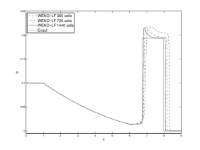
(a) WENO-LF

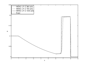
(b) WENO-LF-C

Figure 12: Internal energy plots for the Leblanc shock-tube experiment at $T=6$ using WENO-LF with and without the $C$-equation.

8 Concluding Remarks

We have presented a localized space-time smooth artificial viscosity algorithm, the C-method, and have demonstrated its efficacy on a variety of classical one-dimensional shock-tube problems. As compared to more established procedures, the C-method has been shown to be highly competitive with regards to accuracy and stability, while being relatively easy to implement. Because of its simplicity, the C-method can readily be extended to multiple space-dimensions and/or utilized in reactive-flow simulations. Of value to reactive flows is the localized smooth diffusion provided by the C-method; specifically, the function $C$ can be used to actively influence various mixing-rate-limited reactions occurring near sharp boundaries.

In the future, the gradient-based source term used in the current implementation of the C-method may be combined with a noise-indicator that turns off the current gradient-based source term when it is not needed. Such noise-indicators require a very high-order scheme compatible with DG or 11th-order WENO to name just two examples. By projecting the solution onto a suitable basis, the noise-indicator would activate when small-scale coefficients of this basis do not have sufficient decay; in turn, an indicator function, localized about the region of noise, would activate and force the C equation. This approach is taken in [28], but without any gradient-based forcing functions like our function $G$ or $G_{comp}$.

For example, after the rapid initial growth of the internal energy field in the Leblanc shock-tube problem, this field is essentially representative of the advection of a square-wave. Thus, after initial growth, the gradient-based source term in the C equation for energy could be deactivated leading to less diffusion in the downstream contact discontinuity; simultaneously, the noise-indicator would activate if small-scale instabilities were to set in.

But, for more general problems, the impact of the activation/deactivation of the source term in the C-method on numerical accuracy is not entirely obvious and is left for future research.

References

- [1] A. Harten, B. Engquist, S. Osher, S. R. Chakravarthy, Uniformly high-order accurate essentially non-oscillatory schemes, III, Journal of Computational Physics 71 (1987) 231 – 303.
- [2] C.-W. Shu, S. Osher, Efficient implementation of essentially non-oscillatory shock-capturing schemes, Journal of Computational Physics 77 (1988) 439 – 471.
- [3] C.-W. Shu, S. Osher, Efficient implementation of essentially non-oscillatory shock-capturing schemes, II, Journal of Computational Physics 83 (1989) 32 – 78.
- [4] X.-D. Liu, S. Osher, T. Chan, Weighted essentially non-oscillatory schemes, Journal of Computational Physics 115 (1994) 200–212.
- [5] G.-S. Jiang, C.-W. Shu, Efficient implementation of weighted ENO schemes, Journal of Computational Physics 126 (1996) 202–228.
- [6] B. V. Leer, Towards the ultimate conservative difference scheme. V. A second-order sequel to Godunov’s method, Journal of Computational Physics 32 (1979) 101 – 136.
- [7] P. Colella, A direct eulerian MUSCL scheme for gas dynamics, SIAM Journal on Scientific and Statistical Computing 6 (1985) 104–117.
- [8] H. T. Huynh, Accurate upwind methods for the Euler equations, SIAM Journal on Numerical Analysis 32 (1995) 1565–1619.
- [9] P. Colella, P. R. Woodward, The piecewise parabolic method (PPM) for gas-dynamical simulations, Journal of Computational Physics 54 (1984) 174 – 201.
- [10] J. A. Greenough, W. J. Rider, A quantitative comparison of numerical methods for the compressible Euler equations: fifth-order WENO and piecewise-linear Godunov, Journal of Computational Physics 196 (2004) 259 – 281.
- [11] R. Liska, B. Wendroff, Comparison of several difference schemes on 1D and 2D test problems for the Euler equations, SIAM J. Sci. Comput 25 (2003) 995–1017.
- [12] J. J. Quirk, A contribution to the great Riemann solver debate, Int. J. Num. Methods Fluids 18 (1994) 555–574.
- [13] P. Colella, P. R. Woodward, The numerical simulation of two-dimensional fluid flow with strong shocks, Journal of Computational Physics 54 (1984) 115 – 173.
- [14] A. Majda, S. Osher, Propagation of error into regions of smoothness for accuracte difference approximations to hyperbolic equations, Communications on Pure and Applied Mathematics 30 (1977) 671–705.
- [15] M. Crandall, A. Majda, The method of fractional steps for conservation laws, Numerische Mathematik 34 (1980) 285–314.
- [16] G.-S. Jiang, E. Tadmor, Nonoscillatory central schemes for multidimensional hyperbolic conservation laws, SIAM J. Sci. Comput 19 (1998) 1892–1917.
- [17] C. Hu, C.-W. Shu, Weighted essentially non-oscillatory schemes on triangular meshes, Journal of Computational Physics 150 (1999) 97–127.
- [18] R. D. Richtmyer, Proposed numerical method for calculation of shocks , LANL Report, LA- 671 (1948) 1–18.
- [19] J. von Neumann, R. D. Richtmyer, A method for the numerical calculation of hydrodynamic shocks, Journal of Applied Physics 21 (1950) 232 –237.
- [20] P. Lax, B. Wendroff, Systems of conservation laws, Comm. Pure Appl. Math. 13 (1960) 217–237.
- [21] A. Lapidus, A detached shock calculation by second-order finite differences, Journal of Computational Physics 2 (1967) 154 – 177.
- [22] R. A. Gentry, R. E. Martin, B. J. Daly, An Eulerian differencing method for unsteady compressible flow problems, J. Computational Physics 1 (1966) 87–118.
- [23] F. H. Harlow, A. A. Amsden, A numerical fluid dynamics calculation method for all flow speeds, J. Computational Physics 8 (1971) 197–213.
- [24] T. J. R. Hughes, M. Mallet, A new finite element formulation for computational fluid dynamics: IV. A discontinuity-capturing operator for multidimensional advective-diffusive systems, Computer Methods in Applied Mechanics and Engineering 58 (1986) 329 – 336.
- [25] F. Shakib, T. J. R. Hughes, Z. Johan, A new finite element formulation for computational fluid dynamics: X. The compressible Euler and Navier-Stokes equations, Computer Methods in Applied Mechanics and Engineering 89 (1991) 141 – 219.
- [26] J.-L. Guermond, R. Pasquetti, Entropy-based nonlinear viscosity for Fourier approximations of conservation laws, C.R. Acad. Sci. Paris 346 (2008) 801–806.
- [27] P.-O. Persson, J. Peraire, Sub-cell shock capturing for discontinuous Galerkin Methods, Tech. rep., AIAA (2006).
- [28] G. E. Barter, D. L. Darmofal, Shock capturing with PDE-based artificial viscosity for DGFEM: Part I. Formulation, Journal of Computational Physics 229 (2010) 1810 – 1827.
- [29] R. Löhner, K. Morgan, J. Peraire, A simple extension to multidimensional problems of the artificial viscosity due to Lapidus, Communications in Applied Numerical Methods 1 (1985) 141–147.
- [30] H. Nessyahu, E. Tadmor, Nonoscillatory central schemes for hyperbolic conservation laws, Journal of Computational Physics 87 (1990) 408–463.
- [31] W. J. Rider, J. A. Greenough, J. R. Kamm, Accurate monotonicity-and extrema-preserving methods through adaptive nonlinear hybridizations, Journal of Computational Physics 225 (2007) 1827–1848.
- [32] E. F. Toro, Riemann solvers and numerical methods for fluid dynamics, Springer-Verlay Berling Heidelberg, 2009.
- [33] R. J. DiPerna, Convergence of approximate solutions to conservation laws, Archive for Rational Mechanics and Analysis 82 (1983) 27–70.
- [34] P.-L. Lions, B. Perthame, P. E. Souganidis, Existence and stability of entropy solutions for the hyperbolic systems of isentropic gas dynamics in Eulerian and Lagrangian coordinates, Comm. Pure Appl. Math. 49 (6) (1996) 599–638.
- [35] S. Bianchini, A. Bressan, Vanishing viscosity solutions of nonlinear hyperbolic systems, Annals of Mathematics. Second Series 161 (2005) 223–342.
- [36] T. A. B.E. Robertson A.V. Kravtsov N.Y. Gnedin, D. Rudd, Computational Eulerian hydrodynamics and Galilean invariance, Mon. Not. R. Astron. Soc. 401 (4) (2010) 2463–2476.
- [37] T. W. Roberts, The behavior of flux difference splitting schemes near slowly moving shock waves, Journal of Computational Physics 90 (1990) 141–160.
- [38] K. N. Chueh, C. C. Conley, J. A. Smoller, Positively invariant regions for systems of nonlinear diffusion equations, Indiana University Mathematics Journal 26 (1977) 373–392.
- [39] S. Larsson, V. Thomée, Partial differential equations with numerical methods, Springer-Verlay Berling Heidelberg, 2003.
- [40] B. P. Leonard, The ULTIMATE conservative difference scheme applied to unsteady one-dimensional advection, Comput. Methods Appl. Mech. Engrg. 88 (1991) 17–74.
- [41] A. Harten, S. Osher, Uniformly high-order accurate nonoscillatory schemes. I, SIAM Journal on Numerical Analysis 24 (1987) pp. 279–309.
- [42] G. Sod, A survey of several finite difference methods for systems of nonlinear hyperbolic conservation laws, Journal of Computational Physics 27 (1978) 1 – 31.
- [43] J. S. Hesthaven, T. Warburton, Nodal discontinuous Galerkin methods, algorithms, analysis and applications, Vol. 54 of Texts in Applied Mathematics, Springer, 2008.
- [44] W. Liu, J. Cheng, C.-W. Shu, High-order conservative Lagrangian schemes with Lax-Wendroff type time discretization for the compressible Euler equations, Journal of Computational Physics 228 (2009) 8872–8891.
- [45] R. Loubère, M. Shashkov, A subcell remapping method on staggered polygonal grids for arbitrary-Lagrangian-Eulerian methods, Journal of Computational Physics 209 (2005) 105–138.