Nonlinear dynamo in a short Taylor-Couette setup

Abstract.

It is numerically demonstrated by means of a magnetohydrodynamics code that a short Taylor-Couette setup with a body force can sustain dynamo action. The magnetic threshold is comparable to what is usually obtained in spherical geometries. The linear dynamo is characterized by a rotating equatorial dipole. The nonlinear regime is characterized by fluctuating kinetic and magnetic energies and a tilted dipole whose axial component exhibits aperiodic reversals during the time evolution. These numerical evidences of dynamo action in a short Taylor-Couette setup may be useful for developing an experimental device.

1. Introduction

Still a century after Larmor suggested that dynamo action can be a source of magnetic field in astrophysics, the exact mechanism by which a fluid dynamo can be put in action in astrophysical bodies remains an open challenge. In addition to the numerous analytical and numerical studies that have been done since Larmor’s work, it is only recently that fluid dynamos have been produced experimentally [4, 13, 12]. These experimental dynamos have been helpful in particular to explore the nonlinear saturation regime. For instance, the dynamo produced in the Cadarache experiment [12] has an axial dipolar component and exhibits polarity reversals that are not unlike those observed in astronomical dynamos. The design of this experiment, however, has peculiar features that distinguishes it from natural dynamos. The most notable one is that the flow motion is induced by counter-rotating impellers. This driving mechanism induces an unrealistic differential rotation in the equatorial plane and produces a large turbulent dissipation. Even with a mechanical power injection close to 300 kW, the magnetic Reynolds number of the flow of liquid sodium hardly reaches $R_{\text{\rm m}}=45$. Another peculiarity of this experiment is that dynamo action has not yet been obtained by using blades made of steel. The dynamo threshold has been reached at $R_{\text{\rm m}}=32$ by using blades made of soft iron instead. The objective of the present work is to investigate an alternative driving mechanism that shares the fundamental symmetry properties of natural dynamos, i.e., axisymmetry and equatorial symmetry (so-called $\text{SO}(2)$-$\text{Z}2$ symmetry). The Taylor-Couette geometry is a natural candidate for this purpose, since this configuration is already known to produce dynamos both in axially periodic geometries [15] and in finite vessels of large aspect ratio [7]. We examine in the present paper the dynamo capabilities of Taylor-Couette flows in vessels of small aspect ratio, and we compare the results obtained in this setting with those from more popular spherical dynamos [3].

The paper is organized as follows. The formulation of the problem and the physical setting of the Taylor-Couette configuration under consideration are described in §2. The formulation of the problem and the physical setting of the Taylor-Couette configuration under consideration are described in §2. Three types of flows are considered in the paper and are discussed in §3. These flows are the standard Taylor-Couette flow driven by viscous stresses, a manufactured Taylor-Couette flow, and an optimized flow driven by a body force that models rotating blades attached to the lids. Two kinematic dynamo configurations are investigated in §4. It is found that the poloidal to toroidal ratio of the velocity field generated by viscous driving only (standard Taylor-Couette) is not large enough to generate a dynamo at $R_{\text{\rm m}}\leq 200$. Dynamo action is obtained by using the strengthen Taylor-Couette flow and the forced Taylor-Couette flow. In both cases the poloidal to toroidal ratio of the velocity field is close to one. A nonlinear dynamo obtained with the forced Taylor-Couette flow is described in §5. In the early linear phase of the dynamo, the magnetic field at large distance is dominated by an equatorial rotating dipole. In the established nonlinear regime, an axial axisymmetric component of the magnetic dipole is excited and exhibits aperiodic reversals. Concluding remarks are reported in §6.

2. Formulation of the problem

2.1. The physical setting

We consider an incompressible conducting fluid of constant density $\rho$ and constant kinematic viscosity $\nu$. This fluid is contained between two coaxial cylinders of height $L_{z}$. The radius of the inner cylinder is $R_{i}$ and that of the outer one is $R_{o}$. The inner cylinder is composed of a solid conducting material. The inner cylindrical wall and the top and bottom lids corotate at angular velocity $\Omega_{i}$. The outer cylindrical wall is motionless. The inner solid core may rotate or not, i.e., the inner core and the inner cylindrical wall may have different angular velocities. The conductivity of the fluid and inner solid is assumed to be constant and is denoted $\sigma_{0}$. The magnetic permeability $\mu_{0}$ is assumed to be constant in the entire space.

Let ${\mathcal{U}}$ be a reference velocity scale yet to be defined. We then consider the following reference scales for length, ${\mathcal{L}}=R_{o}-R_{i}$, magnetic field, ${\mathcal{H}}={\mathcal{U}}\sqrt{\rho/\mu_{0}}$, and pressure, ${\mathcal{P}}=\rho{\mathcal{U}}^{2}$. The non-dimensional parameters of the system are the kinetic Reynolds number, $R_{\text{\rm e}}$, the magnetic Reynolds number, $R_{\text{\rm m}}$, the radius ratio $\eta$, and the aspect ratio $\Gamma$:

(2.1) $$R_{\text{\rm e}}=\frac{{\mathcal{U}}{\mathcal{L}}}{\nu},\quad R_{\text{\rm m}}=\mu_{0}\sigma_{0}{\mathcal{U}}{\mathcal{L}},\quad\eta=\frac{R_{i}}{R_{o}},\quad\Gamma=\frac{L_{z}}{{\mathcal{L}}}.$$

To limit the number of geometrical parameters, we restrict ourselves in this paper to $\eta=0.5$ and $\Gamma=2$. Abusing the notation, this immediately implies that $R_{i}=1$ and $R_{o}=2$ in non-dimensional units. We did not explore other aspect ratios (see for example [14, 1, 11, 9] for short aspect ratios and different angular velocities). The conducting domain $\Omega_{c}$ is partitioned into its fluid part enclosed between the two walls, $\Omega_{cf}$, and its solid part enclosed in the inner cylinder, $\Omega_{cs}$. Using non-dimensional cylindrical coordinates $(r,\theta,z)$, we have $\Omega_{cf}=[1,2]{\times}[0,2\pi){\times}[-1,1]$ and $\Omega_{cs}=[0,1]{\times}[0,2\pi){\times}[-1,1]$. The conducting material is embedded in a non-conducting region denoted $\Omega_{v}$, which we refer to as the vacuum region.

The non-dimensional set of equations that we consider is written as follows in the conducting material:

(2.2) $$\partial_{t}{\bf u}+({\bf u}{\cdot}\nabla){\bf u}+\nabla p = \frac{1}{R_{\text{\rm e}}}{\boldsymbol{{\Delta}}}{\bf u}+(\nabla{\times}{\bf H}^{c}){\times}{\bf H}^{c}+{\bf f}_{I}$$

(2.3) $$\nabla\!{\cdot}{\bf u} = 0$$

(2.4) $$\partial_{t}{\bf H}^{c}-\nabla{\times}({\bf u}\times{\bf H}^{c}) = \frac{1}{R_{\text{\rm m}}}{\boldsymbol{{\Delta}}}{\bf H}^{c}$$

(2.5) $$\nabla\!{\cdot}{\bf H}^{c} = 0,$$

where ${\bf u}$, $p$, and ${\bf H}^{c}$ are the velocity field, pressure, and magnetic field, respectively. The magnetic field in ${\Omega_{v}}$ is assumed to derive from a harmonic scalar potential: ${\bf H}^{v}=\nabla\phi$, ${\Delta}\phi=0$. The transmission conditions across the interface separating the conducting and nonconducting material are such that the tangent components of the magnetic and electric fields are continuous (see [6]).

We consider three different settings: (i) The incompressible Navier-Stokes setting (${\bf H}^{c}=0$); (ii) The Maxwell or kinematic dynamo setting; (iii) The nonlinear magnetohydrodynamics setting (MHD). In the Navier-Stokes setting, ${\bf H}^{c}$ is set to zero in the Lorentz force and the induction equation is not solved. The source term ${\bf f}_{I}$ is an ad hoc body force that models blades fixed at the endwalls, see §3.3. When ${\bf f}_{I}=0$, the viscous stress induced by the rotating walls is the only source of momentum, see §3.1. In the Maxwell setting, only the induction equation is solved assuming that some ad hoc velocity field ${\bf u}$ is given. In the MHD setting, the full set of equations is solved.

Since the definition of the reference velocity in similar dynamo configurations may be different (velocity at a given point, maximal speed in the flow, etc.), we introduce the root mean square (rms) velocity to facilitate comparisons:

(2.6) $${\mathcal{U}}^{*2}=\frac{1}{\text{vol}(\Omega_{cf})}\int_{\Omega_{cf}}\|{\bf u}({\bf x},t)\|^{2}\text{d}{\bf x},$$

where the dimensionless fluid volume is $\text{vol}(\Omega_{cf})=6\pi$ in the present case.

2.2. Numerical details

The code (SFEMaNS) that we have developed solves the coupled Navier-Stokes and Maxwell equations in the MHD limit in heterogeneous axisymmetric domains composed of conducting and nonconducting regions by using a mixed Fourier/Lagrange finite element technique. Continuous Lagrange Finite elements are used in the meridian plane and Fourier modes are used in the azimuthal direction. Parallelization is done with respect to the Fourier modes. Continuity conditions across interfaces are enforced using an interior penalty technique [6, 7]. SFEMaNS can account for discontinuous electrical conductivity and magnetic permeability distributions [5, 8]. The magnetic field in the nonconducting regions is assumed to derive from a scalar magnetic potential, i.e., the configurations that we model are such that there is some mechanism that ensures that the circulation of the magnetic field along any path in the insulating medium is zero (this happens for instance when the vacuum is simply connected). The velocity field in $\Omega_{cf}$ and the magnetic field in $\Omega_{c}$ are approximated using continuous ${\mathbb{P}}_{2}$ polynomials, and the pressure field in $\Omega_{cf}$ is approximated using continuous ${\mathbb{P}}_{1}$ polynomials. In the vacuum $\Omega_{v}$, the magnetic potential $\phi$ is approximated using continuous ${\mathbb{P}}_{2}$ polynomials. Typical characteristics of the meshes in the meridian section of all the cases studied in this paper are summarized in Table 1.

Run	$\Delta x$	$\Delta t$	$np(P)$	$np(V)$	$np(H)$	$np(\phi)$	M
§3.1	$1/100$	0.025	5911	23341	-	-	8
§3.3, §3.2	$1/100$	0.025	5911	23341	-	-	12
§4.1, §4.2	$1/100$	0.005	5911	23341	29821	14041	4
§5	$1/100$	0.005	5911	23341	29821	14041	32

Table 1. Characteristics of the runs: $\Delta x$ is the quasi-uniform meshsize in $\Omega_{c}$; $\Delta t$ is the timestep; $np(P)$ is the number of ${\mathbb{P}}_{1}$ nodes for the pressure field in $\Omega_{cf}$; $np(V)$ is the number of ${\mathbb{P}}_{2}$ nodes for the velocity field in $\Omega_{cf}$; $np(H)$ is the number of ${\mathbb{P}}_{2}$ nodes for the magnetic field in $\Omega_{c}$; $np(\phi)$ is the number of ${\mathbb{P}}_{2}$ nodes for the magnetic potential in $\Omega_{v}$. The numbers $np(P)$, $np(V)$, $np(H)$ refer only to the meridian section. The total number of grid points for each unknown $Y$ is obtained by multiplying $np(Y)$ by 2 times the number of Fourier modes, $M$, minus one.

The performance of SFEMaNS has been validated on various kinematic and nonlinear dynamo configurations. In particular, a study of two Taylor-Couette setups using SFEMaNS is reported in [7]. In the first case $\Gamma=4$, $\eta=0.5$, and $z$-periodicity is assumed; in the second case $\Gamma=2\pi$, $\eta=0.5$ and the vessel is finite, i.e., no $z$-periodicity is assumed and the vessel is closed at both ends. In both cases the inner wall rotates, but the outer wall and the two endwalls (when present) are motionless. The self-consistent saturated dynamo found in [15] in the $z$-periodic case has been reproduced in [7], and a new nonlinear dynamo has been found in the finite vessel at $R_{\text{\rm e}}=120,\,R_{\text{\rm m}}=240$. The behaviors of the $z$-periodic and finite-vessel dynamos, as observed in [7], significantly differ. After some transient, the kinetic and magnetic energies of the $z$-periodic dynamo converge to a stationary value. The final nonlinear MHD state is a steady rotating wave resulting from the balance between the driving effect of the viscous shear and the braking effect of the Lorentz force. The nonlinear dynamo action found in the finite vessel shows a different behavior in which the spatial symmetry about the equatorial plane (or mid-plane) of the velocity and magnetic fields plays a key role. The dynamo is cyclic in time and the fields rotate rigidly with modulated amplitude. In these two cases (periodic and finite extension), the wavelength of the magnetic eigenvector is about twice that of the flow; as a result, the velocity field in the median plane of a single magnetic structure is directed inwards. This feature is shared by the spherical kinematic dynamos studied in [3]. It is reported in [3] that the lowest critical magnetic Reynolds number is obtained when the velocity field forms two poloidal cells that flow inwards in the equatorial plane. Note in passing that the two numerical experiments reported in [7] clearly confirm that assuming periodicity or enforcing finite boundary conditions give rise to dynamos with fundamentally different behaviors, i.e., assuming periodicity or ad hoc boundary conditions for the sake of numerical convenience may have nontrivial consequences. The series of observations above have led us to investigate more thoroughly the Taylor-Couette configuration with aspect ratio $\Gamma=2$.

3. Hydrodynamic forcing

Since a number of dynamo studies have shown that the ratio of poloidal to toroidal speed should be close to unity to obtain the lowest critical magnetic Reynolds number, it is important to control this ratio. We describe in this section the mechanisms that we use to optimize the velocity field for dynamo action.

3.1. Taylor-Couette flow (viscous driving only)

When the aspect ratio is about 2 and the kinematic Reynolds number is moderate, two counter-rotating poloidal cells form with a toroidal angular velocity oriented in the same direction as that of the inner cylinder. In order to enforce the equatorial jet to flow inwards, we let the lids of the vessel rotate with the angular velocity of the inner cylinder and we keep the outer cylinder motionless. Note that it is important to have the lids and the inner cylindrical wall of the vessel to corotate; this makes the equatorial jet flow inwards and makes the overall velocity filed similar to the spherical flows that are known to yield dynamo action [3].

We define the velocity reference scale to be

(3.1) $${\mathcal{U}}=\Omega_{i}R_{i},$$

when the only source of momentum is the viscous stress at the boundary.

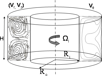
Figure 1. Taylor-Couette flow ${\mathcal{V}}_{0}$, $\Gamma=2$, $R_{\text{\rm e}}=120$. The angular velocity of the lids and the inner cylinder is $\Omega_{i}=1$; the outer cylinder is motionless. A radial jet flows inward at the equator. Represented are the poloidal flow (vectors and streamlines) $-0.2\leq V_{r}\leq 0.3$, and $-0.25\leq V_{z}\leq 0.25$, and the toroidal (or azimuthal) flow $0.25\leq V_{\theta}\leq 2$ (every 0.25).

At $R_{\text{\rm e}}=120$ in the Navier-Stokes regime, the flow is steady, and forms the expected two toroidal cells invariant under the $\text{SO}(2)$-$\text{Z}2$ symmetry, i.e., axisymmetric and symmetric with respect to the equatorial plane, see Figure 1. This flow, henceforth generically referred to as ${\mathcal{V}}_{0}$, is characterized by its rms velocity, $V_{0}^{*}$, defined as follows:

$$V_{0}^{*2}=V_{0p}^{*2}+V_{0t}^{*2}=\frac{1}{\text{vol}(\Omega_{cf})}\int_{{\Omega_{cf}}}(V_{r}^{2}+V_{z}^{2})\text{d}{\bf x}+\frac{1}{\text{vol}(\Omega_{cf})}\int_{{\Omega_{cf}}}V_{\theta}^{2}\text{d}{\bf x},$$

where $V_{0p}^{*}$ and $V_{0t}^{*}$ are the rms poloidal and toroidal velocities of the reference hydrodynamic flow, respectively, and $\text{vol}(\Omega_{cf})=6\pi$ is the volume of the vessel. Our computations give $V_{0}^{*}=0.272$; this value is significantly lower than the maximum speed at the rim of the endwalls which is equal to $2$. The poloidal to toroidal ratio is $\Lambda_{0}=V_{0p}^{*}/V_{0t}^{*}=0.235$.

We have verified that the flow ${\mathcal{V}}_{0}$ is stable with respect to non-axisymmetric perturbations supported on the Fourier modes $m=1,\cdots,7$ at $R_{\text{\rm e}}=120$. The velocity field ${\bf V}_{0}$ together with a sketch of the setup is shown in Figure 1. This reference flow is used in §4.1 to perform kinematic dynamo simulations .

3.2. A modified Taylor-Couette flow

In order to perform kinematic dynamo simulations with a velocity field that has a poloidal to toroidal ratio that can be controlled easily, we construct an ad hoc field based on ${\mathcal{V}}_{0}$. We use the poloidal and toroidal components of the vector field ${\bf V}_{0}$ to define a kinematic field, ${\bf V}_{\epsilon}$, with a pre-assigned poloidal to toroidal ratio as follows:

(3.2) $${\bf V}_{\epsilon}=\frac{\epsilon}{\alpha(\epsilon)}{\bf V}_{0p}+\frac{1}{\alpha(\epsilon)}{\bf V}_{0t}.$$

The normalization is done so that the rms of ${\bf V}_{\epsilon}$ is the same as that of ${\bf V}_{0}$. This gives

(3.3) $$\alpha^{2}(\epsilon)=\frac{1+\epsilon^{2}\Lambda_{0}^{2}}{1+\Lambda_{0}^{2}},\qquad\Lambda(\epsilon)=\epsilon\Lambda_{0}.$$

Since the toroidal component of the velocity at the inner cylinder is equal to $1/\alpha(\epsilon)$, the angular velocity of the inner wall is $\Omega_{i}=1/\alpha(\epsilon)$, and this also means that the reference velocity scale is

(3.4) $${\mathcal{U}}=\alpha(\epsilon)\Omega_{i}R_{i}.$$

Although the vector field ${\bf V}_{\epsilon}$ is not a solution of the Navier-Stokes equations, it is nevertheless solenoidal. This flow is henceforth generically referred to as ${\mathcal{V}}_{\epsilon}$. Computations have been done (see §4.1) for the values of $\epsilon$ reported in Table 2. The quantity denoted $V_{\max}$ in Table 2 is the maximum of the velocity modulus; $V_{\max}$ depends on $\epsilon$.

$\epsilon$	1	3	4	5	6	6.5	8	10	12	16
$\alpha(\epsilon)$	1	1.19	1.34	1.50	1.69	1.78	2.08	2.49	2.92	3.80
$\Lambda(\epsilon)$	0.235	0.71	0.94	1.18	1.41	1.53	1.89	2.36	2.83	3.77
$V_{\max}$	2.00	1.67	1.49	1.32	1.20	1.21	1.23	1.25	1.26	1.27

Table 2. Modified Taylor-Couette flow: normalization factor $\alpha(\epsilon)$, poloidal to toroidal ratio $\Lambda(\epsilon)$ and maximum of the velocity modulus $V_{\max}$.

3.3. Forced Taylor-Couette flow (viscous driving plus body force)

A number of dynamo studies have shown that the ratio of poloidal to toroidal speed should be close to unity to obtain a low critical magnetic Reynolds number. Viscous driving by the rotating walls yields a value for this ratio that is not close to unity ($\Lambda_{0}=0.235$ at $R_{\text{\rm e}}=120$, see section above). At low Reynolds numbers, the flow is steady and axisymmetric. It is relatively easy to vary the relative amplitude of the toroidal component in experimental setups by using blades fixed to the corotating endwalls to act as centrifugal pumps. This configuration, however, is difficult to implement in a computer code. In order to better control the poloidal to toroidal ratio in our simulations, we have chosen to model the toroidal driving by a body force. The action of blades on the top and bottom lids is modeled by an ad hoc axisymmetric divergence-less force given in dimensional form as follows:

(3.5) $${\bf f}_{I}(r,z)=\begin{cases}\displaystyle\rho\frac{A}{r}{\mathcal{U}}^{2}{\bf e}_{r}&\text{if $0.8\leq|z|\leq 1$ and $1.2\leq r\leq 1.8$}\\ 0&\text{otherwise},\end{cases}$$

where the non-dimensional parameter $A$ has been tuned to optimize the poloidal to toroidal ratio. Note that (3.5) defines the reference velocity ${\mathcal{U}}$. The resulting velocity field is denoted ${\bf V}_{I}$ and the flow is generically called ${\mathcal{V}}_{I}$.

We have found that using $A=2.5$ at $R_{\text{\rm e}}=120$ gives $\Lambda_{I}=V_{Ip}^{*}/V_{It}^{*}=1.04$ and the rms velocity is $V_{I}^{*}=0.219$. We have observed that the azimuthal velocity in the vicinity of the inner radius is close to $0.55$; hence, to reduce the viscous boundary layer at the inner wall and endwalls, we have set the dimensionless angular velocity to $\Omega_{i}=0.55$. The steady axisymmetric flow ${\mathcal{V}}_{\text{I}}$ is shown in Figure 2, (see Figure 1 for a comparison with the pure Taylor-Couette flow).

(a) Poloidal flow, $\theta=\pi$

(b) Toroidal flow, $\theta=0$

Figure 2. Forced Taylor-Couette flow ${\mathcal{V}}_{\text{I}}$, $\Gamma=2$, $R_{\text{\rm e}}=120$, and $A=2.5$. The lids and the inner cylinder rotate with angular speed $\Omega_{i}=0.55$; the outer cylinder is motionless. A radial jet flows inwards at the equator. Represented are the poloidal flow (vectors and streamlines), $-0.7\leq V_{r}\leq 1.4$, $-1.1\leq V_{z}\leq 1.1$, and the toroidal (or azimuthal) flow, $0\leq V_{\theta}\leq 1.6$ (10 levels)

We have verified, by performing nonlinear Navier-Stokes simulations, that the flow ${\mathcal{V}}_{I}$, at $Re=120$, is stable with respect to three-dimensional perturbations supported on Fourier modes up to $m=11$. The first hydrodynamic non-axisymmetric instability occurs on the Fourier mode $m=3$ at $R_{\text{\rm e}}=168$. The steady and axisymmetric forced Taylor-Couette flow ${\mathcal{V}}_{\text{I}}$ is used in §4.2 to perform kinematic dynamo simulations.

3.4. Summary

To compare the flows ${\mathcal{V}}_{0}$, ${\mathcal{V}}_{I}$, and ${\mathcal{V}}_{\epsilon}$, we show in Table 3 the following characteristics of these three flows: rms velocity, $V^{*}$; maximum of the velocity modulus in the fluid domain, $V_{\max}$; poloidal to toroidal ratio, $\Lambda$.

Run	$V^{*}$	$V_{\max}$	$\Lambda$
Viscous flow ${\mathcal{V}}_{0}$, §3.1	0.272	2.00	0.235
Modified flow ${\mathcal{V}}_{\epsilon}$, §3.2,§4.1	0.272	(1.20,2.00)	$0.235{\times}\epsilon$
Forced flow ${\mathcal{V}}_{\text{I}}$, §3.3,§4.2,§5	0.219	1.09	1.04

Table 3. Characteristics of the flows ${\mathcal{V}}_{0}$, ${\mathcal{V}}_{\epsilon}$ and ${\mathcal{V}}_{\text{I}}$: $V^{*}$ is the r.m.s. speed; $V_{\max}$ is the maximum of the velocity modulus in the fluid domain; $\Lambda$ is the poloidal to toroidal ratio.

4. Kinematic Dynamos

We evaluate in this section the properties of the kinematic dynamos generated by the flows ${\mathcal{V}}_{\epsilon}$ (viscous driving) and ${\mathcal{V}}_{I}$ (viscous driving plus body force).

4.1. Parametric study of the poloidal to toroidal ratio using ${\mathcal{V}}_{\epsilon}$

We investigate the dynamo properties of the manufactured flow ${\mathcal{V}}_{\epsilon}$ in the kinematic regime, see §3.2. The reference velocity scale is defined in (3.4). To ensure that the velocity is continuous across the solid/fluid interface, the angular velocity of the inner core is set to be $1/\alpha(\epsilon)$. The conductivities of the solid inner core and the fluid are identical.

We perform two studies at $R_{\text{\rm m}}=100$ and $R_{\text{\rm m}}=200$ to determine the optimal weight $\epsilon$ that gives the largest growthrate of the dynamo action in the kinematic regime. The computations are done with SFEMaNS in Maxwell mode. The magnetic field is initialized to some small random values and the growth rate (i.e., the real part of the leading eigenvalue) is computed by running short time simulations for various ratios $\epsilon\in[3,16]$ shown in Table 2. As the vector field ${\bf V}_{\epsilon}$ is axisymmetric, the term $\nabla{\times}({\bf V}_{\epsilon}{\times}{\bf H}^{c})$ cannot transfer energy between the Fourier modes of ${\bf H}^{c}$, i.e., the Fourier modes are uncoupled. The first bifurcation is of Hopf type and the most unstable eigenvector is the Fourier mode $m=1$. The growthrate of the magnetic energy is reported in Figure 3. There is no dynamo action at $R_{\text{\rm m}}=100$. Dynamo action occurs at $R_{\text{\rm m}}=200$ in the range $4.2<\epsilon<15.4$, which corresponds to $1.0<\Lambda(\epsilon)<3.8$. Note that the purely viscous driving, which corresponds to $\epsilon=1$ and $\Lambda_{0}=0.235$, cannot sustain a dynamo at $R_{\text{\rm m}}=100$ and $R_{\text{\rm m}}=200$.

Figure 3. Kinematic dynamo. Growthrate of Fourier mode $m=1$ for the modified Taylor-Couette flow, ${\mathcal{V}}_{\epsilon}$, as a function of $\epsilon$ for $R_{\text{\rm m}}=100$ and $R_{\text{\rm m}}=200$; $\Gamma=2$ and $R_{\text{\rm e}}=120$.

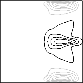
(a) $H_{r}$ at $\theta=0$

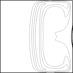
(b) $H_{\theta}$ at $\theta=0$

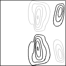
(c) $H_{z}$ at $\theta=0$

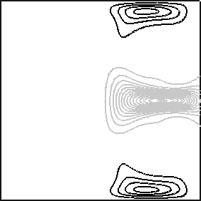
(d) $H_{r}$ at $\theta=\frac{\pi}{2}$

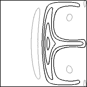
(e) $H_{\theta}$ at $\theta=\frac{\pi}{2}$

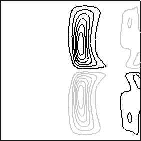
(f) $H_{z}$ at $\theta=\frac{\pi}{2}$

(g) isosurface $\|{\bf H}^{c}\|^{2}$

Figure 4. Kinematic dynamo with flow ${\mathcal{V}}(\epsilon=8)$ at $R_{\text{\rm e}}=120$, $R_{\text{\rm m}}=200$. Magnetic eigenvector for Fourier mode $m=1$. Represented in (a) to (f) are the radial, azimuthal, and vertical components, normalized by the square root of the magnetic energy, in two complementary planes, with $0\leq r\leq 2,\,-1\leq z\leq 1$ (the $z-$axis is on the left): for $\theta=0$, $-0.85\leq H_{r}\leq 0.85$ (every 0.17), $-0.1\leq H_{\theta}\leq 0.68$ (every 0.17) and $-0.85\leq H-z\leq 0.85$ (every 0.17); for $\theta=\frac{\pi}{2}$, $-1\leq H_{r}\leq 3.75$ (every 0.25), $-1\leq H_{\theta}\leq 0.15$ (every 0.25) and $-1.5\leq H_{z}\leq 1.5$ (every 0.25). Represented in (g) is the isosurface $\|{\bf H}^{c}\|^{2}$ ($7\%$ of maximum value) colored by the azimuthal component. Note the $m=1$ structure.

Figure 4 shows the magnetic eigenvector for the Fourier mode $m=1$ at $R_{\text{\rm e}}=120$, $R_{\text{\rm m}}=200$ and $\epsilon_{opt}=8$. This eigenvector is a rigid wave that rotates in the same direction as the inner cylinder and top/bottom lids, and its period of rotation is $T\simeq 870$, i.e., more than 66 rotation periods. Upon introducing the equatorial symmetry operator ${\mathcal{S}}_{\text{Z}2}{\bf H}=(H_{r},\;H_{\theta},\;-H_{z})(r,\theta,-z)$. the magnetic field has the following symmetry property:

(4.1) $${\bf H}^{c}={\mathcal{S}}_{\text{Z}2}{\bf H}^{c}.$$

i.e., the magnetic field has the same symmetry as the velocity field.

Figure 5. Kinematic dynamo of flow ${\mathcal{V}}(\epsilon=6.5)$, $\Gamma=2$, $R_{\text{\rm e}}=120$. Growthrate of the Fourier mode $m=1$ as a function of $R_{\text{\rm m}}$.

We now evaluate the critical magnetic Reynolds number and its minimal value with respect to $\epsilon$. We assume that the growthrate depends smoothly on $R_{\text{\rm m}}$. Upon inspecting Figure 3 we see that the growth rate is maximum for $\epsilon_{opt}\approx 5$ at $R_{\text{\rm m}}=100$ and for $\epsilon_{opt}\approx 8$ ate $R_{\text{\rm m}}=200$. Then, by drawing the line connecting the two maximum points in Figure 3, we observe that this line crosses the horizontal line of zero growth rate in the interval $\epsilon\in[6.5,7]$. We have chosen to explore the value $\epsilon=6.5$, which gives the poloidal to toroidal ratio $\Lambda=1.53$. The growth rate for various magnetic Reynolds numbers in the range $[125,200]$ has been computed. The results are shown in Figure 5. We have found that the critical magnetic Reynolds number for the Fourier mode $m=1$ is $R_{\text{\rm m}}=155$ with $\epsilon=6.5$ and $\Lambda=1.53$.

4.2. Kinematic dynamo in the forced Taylor-Couette setup

We use the steady axisymmetric forced flow, ${\mathcal{V}}_{\text{I}}$, at $R_{\text{\rm e}}=120$ to perform kinematic dynamo computations. The reference velocity scale is defined in (3.5) with $A=2.5$. To determine whether the rotation of the inner solid core has any impact on the dynamo threshold, we have compared growth rates when the solid inner core is motionless and when the inner wall and solid inner core corotate with angular speed $\Omega_{i}$. Whether the inner core rotates or not, the magnetic eigenvector $m=1$ is always the most unstable. We show in Figure 6 the computed growth rates in the two cases in the range $R_{\text{\rm m}}\in[175,200]$. The motion of the inner core does not seem to have a significant influence; in both cases the dynamo threshold is $R_{\text{\rm m}}=180$ for the Fourier mode $m=1$.

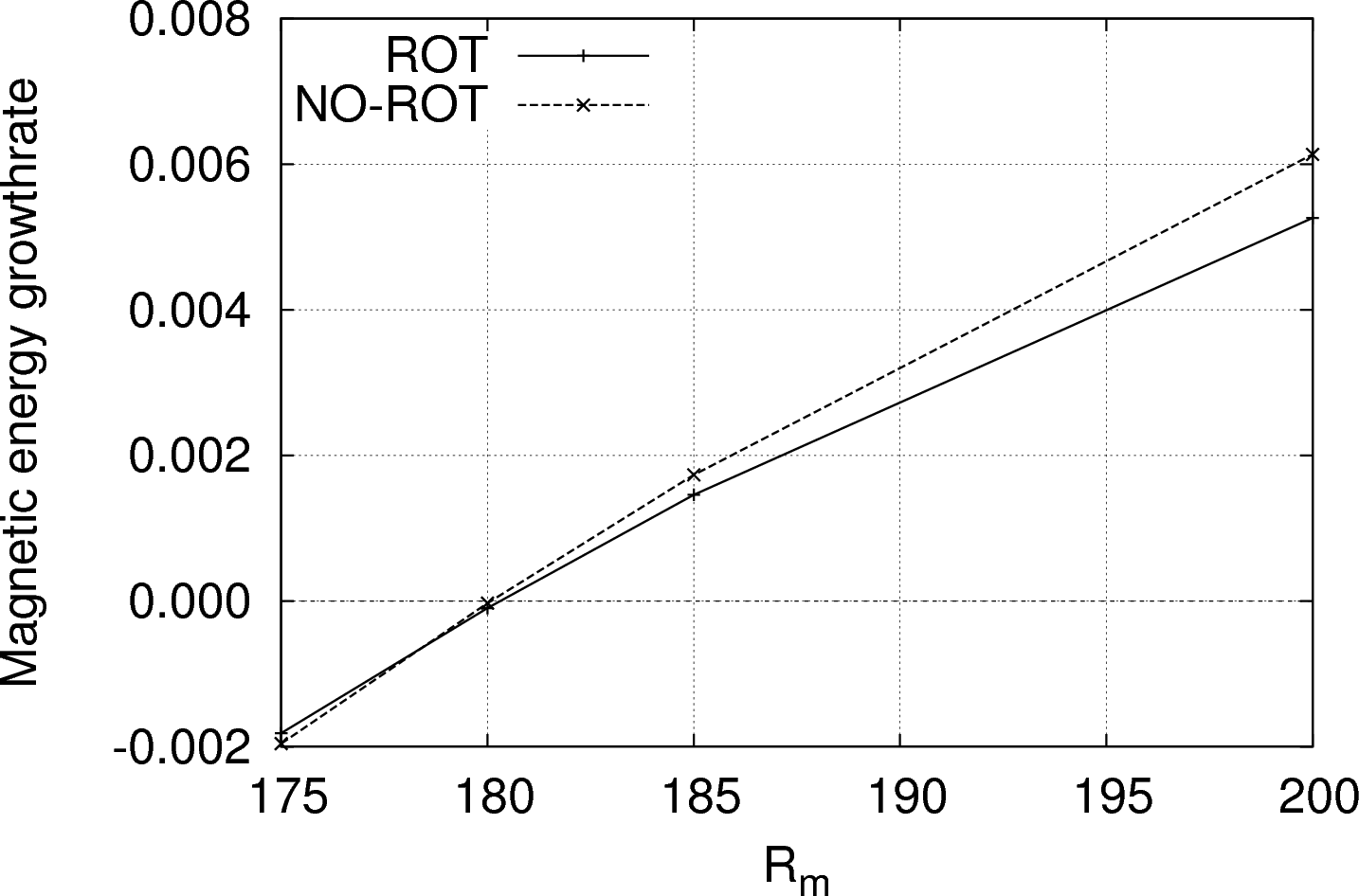
Figure 6. Kinematic dynamo with ${\mathcal{V}}_{I}$ flow, $\Gamma=2$ and $R_{\text{\rm e}}=120$ . Growthrate of the Fourier mode $m=1$ as a function of $R_{\text{\rm m}}$. ROT: rotating inner core; NO-ROT: non-rotating inner core (but inner wall rotates).

The structure of the magnetic eigenvector corresponding to the Fourier mode $m=1$ with a rotating inner core is shown in Figure 7 (at $R_{\text{\rm e}}=120$, $R_{\text{\rm m}}=200$). It is a rigid wave that rotates in the same direction as the inner cylinder and top/bottom lids with period $T\simeq 120$.

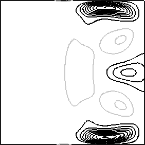
(a) $H_{r}$ at $\theta=0$

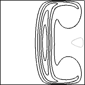
(b) $H_{\theta}$ at $\theta=0$

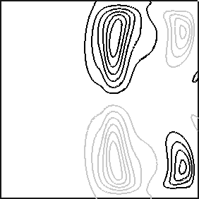
(c) $H_{z}$ at $\theta=0$

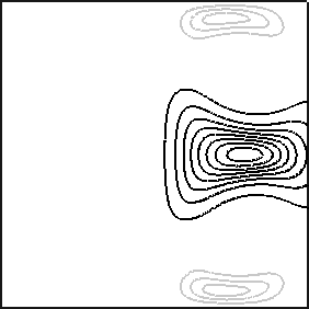
(d) $H_{r}$ at $\theta=\frac{\pi}{2}$

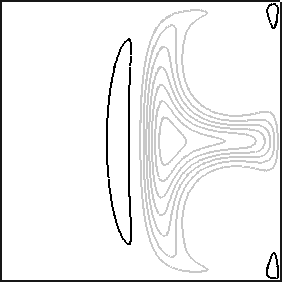
(e) $H_{\theta}$ at $\theta=\frac{\pi}{2}$

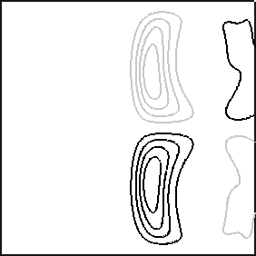
(f) $H_{z}$ at $\theta=\frac{\pi}{2}$

(g) isosurface $\|{\bf H}^{c}\|^{2}$

Figure 7. Kinematic dynamo with flow ${\mathcal{V}}_{I}$ at $R_{\text{\rm e}}=120$, $R_{\text{\rm m}}=200$. Magnetic eigenvector for Fourier mode $m=1$. Represented in (a) to (f) are the radial, azimuthal, and vertical components, normalized by the square root of the magnetic energy, in two complementary planes: for $\theta=0$, $-0.9\leq H_{r}\leq 0.2$ (every 0.1), $-1.4\leq H_{\theta}\leq 0.35$ (every 0.25) and $-0.6\leq H_{z}\leq 0.6$ (every 0.1); for $\theta=\pi/2$, $-2.2\leq H_{r}\leq 0.9$ (every 0.25), $-0.25\leq H_{\theta}\leq 1.75$ (every 0.25) and $-1.25\leq H_{z}\leq 1.25$ (every 0.1). Represented in (g) is the isosurface $\|{\bf H}^{c}\|^{2}$ ($14\%$ of maximum value) colored by the azimuthal component. Note the $m=1$ structure.

5. Nonlinear dynamo action

We report in this section on nonlinear dynamo computations done with the forced Taylor-Couette setup at $R_{\text{\rm e}}=120$ and $R_{\text{\rm m}}=200$.

5.1. Description of the setting

We consider the forced Taylor-Couette setup described in §4.2. The reference velocity scale is defined in (3.5) with $A=2.5$. We perform nonlinear dynamo computations with the parameters $R_{\text{\rm e}}=120$, $R_{\text{\rm m}}=200$. The inner core is kept motionless. We work with 32 azimuthal modes ($m=0,\ldots,31$), and the meridional finite element mesh is the same as in the kinematic runs. The total number of degrees of freedom to be updated at each time step is $11{,}353{,}104$. The initial velocity field is the axisymmetric flow ${\mathcal{V}}_{\text{I}}$ that we computed in the Navier-Stokes regime at $R_{\text{\rm e}}=120$. The initial magnetic seed is the growing Fourier mode $m=1$ obtained in the kinematic computations described in §4.2 at $R_{\text{\rm m}}=200>R_{\text{\rm mc}}=180$.

When dynamo action occurs, the magnetic energy grows exponentially until the Lorentz force is capable of modifying the base flow. This transient phase lasts about 5 rotation periods. When the Lorentz force is strong enough, a new regime settles where the magnetic energy saturates. Nonlinear saturation is a slow process that lasts at least 200 rotation periods (see Figure 11 in [7]). Although SFEMaNS is parallel with respect to the Fourier modes, the volume of computation required by this type of simulation is such that we have not been able to explore other kinematic and magnetic Reynolds numbers within the resources allocated to this project. The nonlinear run presented in this section used about 15600 cumulated CPU hours with 32 processors on an IBM Power 6 cluster.

5.2. Time evolution of the energy

The time evolutions of the kinetic and magnetic energies are reported in Figure 8(a-b), where the kinetic and magnetic energies are defined as follows: $\frac{1}{2}\int_{{\Omega_{cf}}}\|{\bf u}\|^{2}\text{d}{\bf x}$, $\frac{1}{2}\int_{{\Omega_{c}}}\|{\bf H}^{c}\|^{2}\text{d}{\bf x}$, respectively. From $t=0$ to $t=500$ (first transition), the kinetic energy decreases and the magnetic energy grows exponentially with a growthrate similar to that of the kinematic dynamo. Then both the magnetic and the kinetic energies seem to saturate in a first nonlinear regime, $500\lesssim t\lesssim 1100$. During the first transition, the fluid flow loses the axial symmetry, $m=0$, and the magnetic field loses the symmetry associated with the Fourier mode $m=1$. The flow being forced by the Lorentz force $(\nabla{\times}{\bf H}^{c}){\times}{\bf H}^{c}$, the velocity thereby acquires a contribution on the Fourier mode $m=2$. The magnetic field being deformed by the action of the induction term ${\bf u}{\times}{\bf H}^{c}$ acquires a contribution on the Fourier mode $m=3$. The cascade of nonlinear couplings generate even velocity modes, $m=0,2,\ldots$, and odd magnetic modes, $m=1,3,\ldots$ During this transitional phase that consists of populating the Fourier modes, the axisymmetry of the velocity field is broken but the equatorial (mid-plane) symmetry is preserved for both the velocity and the magnetic field.

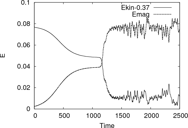
(a) Kinetic (-0.37) and magnetic energies

(b) Splitting of magnetic energy

Figure 8. Nonlinear dynamo in the forced Taylor-Couette setup. (a) Time evolution of kinetic (-0.37) and magnetic energies in the conducting region $0\leq r\leq R_{o}$ and $-\Gamma/2\leq z\leq\Gamma/2$. Panel (b) shows the symmetric and anti-symmetric components of the magnetic energy.

A second nonlinear transition starts at $t=1100$ and lasts until $t=1175$. In this time interval the magnetic energy increases and the kinetic energy decreases. This change of behavior is due to the breaking of the equatorial symmetry. This phenomenon is well illustrated by computing the energy of the symmetric part, $\frac{1}{2}({\bf H}^{c}+{\mathcal{S}}_{\text{Z}2}{\bf H}^{c})$, and anti-symmetric part, $\frac{1}{2}({\bf H}^{c}-{\mathcal{S}}_{\text{Z}2}{\bf H}^{c})$, of the magnetic field. The time evolution of these two quantities is shown in Figure 8(c). The equatorial symmetry breaking is driven by the small even azimuthal modes of the magnetic field as can be seen on Figure 9 (a)(b), especially the magnetic mode $m=2$.

(a) Magnetic energy, $m=0,1,2,3$

(b) Kin. $m=1,\,3$; Mag. $m=0,\,2$

(c) Magnetic energy, $m=0,1,30,31$

Figure 9. Time evolution of different modal energies; (a) magnetic energies $m=0,\,2$ (bottom curves) and $m=1,\,3$ (top curves); (b) kinetic energies $m=1,\,3$ and magnetic energies $m=0,\,2$; (c) magnetic energies $m=1$ (top curve), $m=30,\,31$ (middle curves) and $m=0$.

In the time interval $1175\leq t\leq 1600$, the system enters a second nonlinear regime characterized by large fluctuations and a dynamics dominated by the large Fourier modes. Between $t=1600$ and $t=2200$, we observe a third transition during which the small even modes of the magnetic field increase again until they reach the final saturated state. A third and final nonlinear regime settles beyond $t=2200$. Figure 9(c) shows that the large Fourier modes, exemplified by $m=30$ and $m=31$, basically fluctuate within some asymptotic range for $t>1250$, whereas the small even modes grow until they become energetically significant.

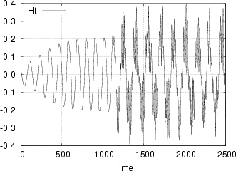
(a) $H_{\theta}(1.2,0,-0.5,t)$

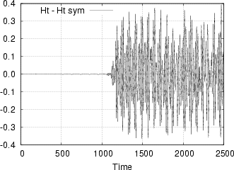
(b) $H_{\theta}(1.2,0,-0.5,t)-H_{\theta}(1.2,0,0.5,t)$

Figure 10. Time series of (a) $H_{\theta}$ at $(r=1.2,\theta=0,z=-0.5)$ and (b) twice the anti-symmetric part of $H_{\theta}$ at $(r=1.2,\theta=0,z=-0.5)$.

We show in Figure 10(a) the time series of the azimuthal component of the magnetic field at the point $(r=1.2,\theta=0,z=-0.5)$. The envelop of the signal first grows then reaches a maximum range. The period of the signal is $T\approx 112.5$; this corresponds to a wave that rotates in the same direction as the inner cylinder and top/bottom lids. More frequencies appear beyond $t=1100$; the signal is the superposition of an oscillation of period $T\approx 150$ and a modulation of period $T_{\text{mod}}\approx 17$, which happens to be of the same order as the wall rotation period $T_{\text{lids}}=2\pi/0.55\approx 11.4$. The breaking of the equatorial symmetry is measured by monitoring the anti-symmetric part of the magnetic field. We show in Figure 10(b) the time evolution of twice the anti-symmetric part of $H_{\theta}$ at $(r=1.2,\theta=0,z=-0.5)$.

5.3. Spatial structure of the dynamo

To have a better understanding of the structure of the velocity and magnetic fields during the three nonlinear regimes identified above, we show in Figure 11 the isosurfaces of the magnetic and kinetic energies at $t=1000$, $t=1400$, and $t=2500$. Since the axisymmetric velocity mode $m=0$ is dominant (see Figure 11(d-f)), we show in Figure 11(g-i) the kinetic energy without its axisymmetric contribution to better distinguish the fine structures. The magnetic field at $t=1000$ is dominated by the odd azimuthal modes (see Figure 11(a)) and resembles the eigenvector shown in Figure 7(g). The velocity field is composed of even modes as can be seen on Figure 11(g), see e.g. the two dark structures that are diametrically opposed. Similar spatial distributions are observed at time $t=1400$ with the addition of smaller scales. At time $t=2500$ the small scale modes are even more apparent, and the magnetic and velocity structures in the fluid domain are more deformed.

Isosurface $\|{\bf H}^{c}\|^{2}$ ($25\%$ of maximum value)

(a) $t=1000$

(b) $t=1400$

(c) $t=2500$

Isosurface $\|{\bf V}\|^{2}$ ($25\%$ of maximum value)

(d) $t=1000$

(e) $t=1400$

(f) $t=2500$

Isosurface $\|{\bf V}\|^{2}$ without the axisymmetric mode $m\,{=}\,0$ ($10\%$ of maximum value)

(g) $t=1000$

(h) $t=1400$

(i) $t=2500$

Figure 11. Nonlinear dynamo at $t=1000$, $t=1400$ and $t=2500$, for $R_{\text{\rm e}}=120$, $R_{\text{\rm m}}=200$: (a-c) isosurface of $\|{\bf H}^{c}\|^{2}$ ($25\%$ of maximum value); (d-f) isosurface of $\|{\bf V}\|^{2}$ ($25\%$ of maximum value); (g-i) isosurface of $\|{\bf V}\|^{2}$ without the axisymmetric mode ($10\%$ of maximum value); color scale proportional to azimuthal component.

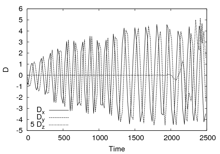
(a) $0\leq t\leq 2500$

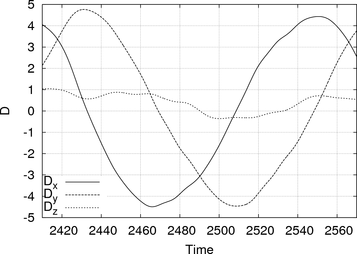
(b) Zoom in $2410\leq t\leq 2570$

Figure 12. Time evolution of the dipolar magnetic moment. Note that the vertical component has been multiplied by 5 in the left panel.

To characterize the long distance influence of the magnetic field, we have recorded the time evolution of the magnetic dipole defined by ${\bf D}=\int_{{\Omega_{c}}}{\bf r}{\times}(\nabla{\times}{\bf H}^{c})\text{d}{\bf x}$. Figure 12 shows the time series of the three Cartesian components of the magnetic dipole in the time interval $0\leq t\leq 2500$. During the first two transitions and nonlinear regimes, i.e., $0\leq t\leq 1600$, the dipolar moment is purely equatorial and rotates at the same frequency as the magnetic field. The axial moment starts to grow at the beginning of the third transition ($t>1600$) and changes sign several times afterward (note that the time series in (a) is under sampled in this range). Figure 12(b) presents a zoom of the time evolution of $D_{z}$ showing two reversals. The magnitude of the quadrupolar moments (data not shown) stay below $10^{-3}$ until $t=1175$, then increase and saturate to values four times smaller than the magnitude of the dipolar moment. Magnetic field lines in the vacuum at $t=2500$ show a pattern characteristics of an equatorial dipole (see Figure 13).

(a) From above

(b) From a perspective point of view

Figure 13. Isosurface of $\|{\bf H}^{c}\|^{2}$ ($25\%$ of maximum value) and magnetic field lines at $t=2500$.

6. Concluding remarks

We have numerically demonstrated that pure viscous driving by smooth rotating walls in a short Taylor-Couette setup does not lead to dynamo action for $R_{\text{\rm m}}\leq 200$ since the poloidal to toroidal ratio of the velocity field is too small. An adjustment of the poloidal to toroidal ratio is needed to achieve dynamo action in the kinematic regime. We have implemented an ad hoc body force to produce a poloidal to toroidal ratio that is of the same order as what is needed in the kinematic simulations to trigger the dynamo action. This force may be thought of as a model for the action of blades fixed to the static or to the rotating walls/lids at convenient angles. This force has also the same symmetry properties as the geodynamo, i.e., the $\text{SO}(2){\times}\text{Z}2$ symmetry (axisymmetry and equatorial symmetry). The critical magnetic Reynolds number of this setup based on the inner cylinder speed $\mu_{0}\sigma\Omega_{i}R_{i}^{2}=0.55{\times}180=99$ is in the range of what has been obtained in the kinematic studies of [3] in a spherical container with the same symmetries. This magnetic Reynolds number is also comparable to what has been reported in [7] for Taylor-Couette simulations in vessels of larger aspect ratios and with pure viscous driving.

A nonlinear simulation has been performed at $R_{\text{\rm e}}=120$, $R_{\text{\rm m}}=200$ over 225 rotation periods. In the early linear phase of the dynamo, the external field is dominated by an equatorial rotating dipole. In the established nonlinear regime, an axial axisymmetric component is excited and exhibits reversals. The relation between the main flow parameters of the time-dependent angle formed by the dipole and the rotation axis calls for further investigations, since it is a basic feature of observed planetary dynamos.

Exploring the feasibility of an experimental fluid dynamo based on the present design will require expertise from many different experimental and numerical fields [10]. To achieve a magnetic Reynolds number equal to $100$ in a flow of liquid sodium requires that the kinematic Reynolds number be of order $10^{7}$. It is well known that such a value corresponds to a highly turbulent flow that can be studied only in experimental facilities, since it is far beyond the capacity of direct numerical simulations. The objective of such experiments should be to recover optimized poloidal and toroidal components after time averaging, which presumably would guide the design of the blades fixed to the endwalls. These experiments would also inform about the power requirements. Using a standard rotation frequency of $50$ Hz, a magnetic Reynolds number of $100$ can be obtained in liquid sodium at $150^{\text{o}}$C with an inner radius of approximatively $18$ cm and an outer radius and height of $36$ cm. This seems feasible since these dimensions are not far from those of the Cadarache experiment [12]. We conjecture however that the power required by this experiment at a given rotation frequency should be smaller, since the turbulence rate induced by co-rotating lids/impellers should be smaller than that of counter-rotating lids/impellers. A dynamo facility presenting similarities with the present proposal is currently investigated by Colgate and collaborators [2]. Their MHD device uses also a Taylor-Couette forcing in a short cylindrical container with size and targeted magnetic Reynolds number similar to those studied in the present paper. There are however differences: the flow in their experiment forms an outwards jet in the equatorial plane and is driven by viscous stresses only. More detailed comparisons of the respective merits of both designs should certainly be instructive.

References

- [1] J. Abshagen, K.A. Cliffe, J. Langenberg, T. Mullin, G. Pfister, and S.J. Tavener. Taylor–Couette flow with independently rotating end plates. Theoretical and Computational Fluid Dynamics, 18:129–136, 2004. 10.1007/s00162-004-0135-3.
- [2] S. A. Colgate, H. Beckley, J. Si, J. Martinic, D. Westpfahl, J. Slutz, C. Westrom, B. Klein, P. Schendel, C. Scharle, T. McKinney, R. Ginanni, I. Bentley, T. Mickey, R. Ferrel, H. Li, V. Pariev, and J. Finn. High magnetic shear gain in a liquid sodium stable Couette flow experiment: A prelude to an - dynamo. Phys. Rev. Lett., 106:175003, Apr 2011.
- [3] M.L. Dudley and R.W. James. Time-dependent kinematic dynamos with stationary flows. Proc. Roy. Soc. London, A425:407–429, 1989.
- [4] A. Gailitis, O. Lielausis, S. Dement’ev, E. Platacis, and A. Cifersons. Detection of a flow induced magnetic field eigenmode in the Riga dynamo facility. Phys. Rev. Lett., 84:4365, 2000.
- [5] A. Giesecke, C. Nore, F. Stefani, G. Gerbeth, J. Léorat, F. Luddens, and J.-L. Guermond. Electromagnetic induction in non-uniform domains. Geophys. Astrophys. Fluid Dyn., 104(5):505–529, 2010.
- [6] J.-L. Guermond, R. Laguerre, J. Léorat, and C. Nore. An interior penalty Galerkin method for the MHD equations in heterogeneous domains. J. Comput. Phys., 221(1):349–369, 2007.
- [7] J.-L. Guermond, R. Laguerre, J. Léorat, and C. Nore. Nonlinear magnetohydrodynamics in axisymmetric heterogeneous domains using a fourier/finite element technique and an interior penalty method. J. Comput. Phys., 228:2739 2757, 2009.
- [8] J.-L. Guermond, J. Léorat, F. Luddens, C. Nore, and A. Ribeiro. Effects of discontinuous magnetic permeability on magnetodynamic problems. J. Comput. Phys., 230:6299–6319, 2011.
- [9] R.E Hewitt, T Mullin, S.J Tavener, M.A.I Khan, and P.D Treacher. Nonlinear vortex development in rotating flows. Philosophical Transactions of the Royal Society A: Mathematical, Physical and Engineering Sciences, 366(1868):1317–1329, 2008.
- [10] J. Léorat and C. Nore. Interplay between experimental and numerical approaches in the fluid dynamo problem. Comptes Rendus Physique, 9:741–748, September 2008.
- [11] F. Marques and J. M. Lopez. Onset of three-dimensional unsteady states in small-aspect-ratio Taylor–Couette flow. Journal of Fluid Mechanics, 561:255–277, 2006.
- [12] R. Monchaux, M. Berhanu, M. Bourgoin, Ph. Odier, M. Moulin, J.-F. Pinton, R. Volk, S. Fauve, N. Mordant, F. Pétrélis, A. Chiffaudel, F. Daviaud, B. Dubrulle, C. Gasquet, L. Marié, and F. Ravelet. Generation of magnetic field by a turbulent flow of liquid sodium. Phys. Rev. Lett., 98:044502, 2007.
- [13] R. Stieglitz and U. Müller. Experimental demonstration of a homogeneous two-scale dynamo. Phys. Fluids, 13:561, 2001.
- [14] S. J. Tavener, T. Mullin, and K. A. Cliffe. Novel bifurcation phenomena in a rotating annulus. Journal of Fluid Mechanics, 229:483–497, 1991.
- [15] A. P. Willis and C. F. Barenghi. A Taylor-Couette dynamo. Astronomy and Astrophysics, 393:339–343, 2002.