Cycles of the logistic map

Abstract

The onset and bifurcation points of the $n$-cycles of a polynomial map are located through a characteristic equation connecting cyclic polynomials formed by periodic orbit points. The minimal polynomials of the critical parameters of the logistic, Hénon, and cubic maps are obtained for $n$ up to 13, 9, and 8, respectively.

I Introduction

Consider the logistic map may ; strogatz :

$$x_{k+1}=f(x_{k})\equiv r\,x_{k}\,(1-x_{k}).$$ (1)

If we iterate Eq. (1) from $k=0$, what does the resulting sequence $x_{0}$, $x_{1}=f(x_{0})$, $x_{2}=f(x_{1})$, $\ldots$ look like? We can visualize the sequence on the cobweb plot, see Fig. 1 for examples. Starting from $(x_{0},x_{0})$ on the diagonal, each vertical arrow takes $(x_{k},x_{k})$ to $(x_{k},y)$, where $y=f(x_{k})=x_{k+1}$; the next horizontal arrow then reflects $(x_{k},y)$ to $(y,y)=(x_{k+1},x_{k+1})$, which starts the next iteration.

Figure 1: Cobweb plot of the logistic map.

Three outcomes are possible: (i) a fixed point, which is a constant (including infinity), e.g., Fig. 1(a); (ii) a periodic cycle, which is a self-repeating pattern, e.g., Figs. 1(b)-(e); or (iii) a chaotic trajectory, e.g., Fig. 1(f). We will focus on the first two cases here.

A fixed point is a solution of $x^{*}=f(x^{*})$. If $x_{0}$ deviates slightly from $x^{*}$ and the sequence still converges to $x^{*}$, we call it stable. For a differentiable $f$, a stable fixed point requires $|f^{\prime}(x^{*})|\leq 1$ to reduce deviations in successive iterations strogatz .

In an $n$-cycle, $n$ is the smallest positive integer that allows $x_{1}=x_{n+1}=f^{n}(x_{1})$, where $f^{n}$ is the $n$th iterate of $f$, e.g., $f^{3}(x)=f(f(f(x)))$. Thus, any $x_{k}$ in an $n$-cycle of $f$ must be a fixed point of $f^{n}$ [the reverse is, however, untrue, for a fixed point of $f^{n}$ can also be a fixed point of $f^{d}$ as long as $d|n$: if $f^{d}(x)=x$, then $f^{n}(x)=f^{d}(\cdots f^{d}(x)\cdots)=x$]. We can therefore classify a cycle as stable or unstable by the corresponding fixed point of $f^{n}$: a stable cycle requires $\big{|}\frac{d}{dx}f^{n}(x_{1})\big{|}\leq 1$, or by the chain rule,

$$\Big{|}f^{\prime}(x_{1})\dots f^{\prime}(x_{n})\Big{|}\leq 1,$$ (2)

where $x_{1}.\ldots,x_{n}$ are the $n$ points within the cycle, or the orbit. Further, the onset and bifurcation points are defined at the loci where $\frac{d}{dx}f^{n}(x_{1})$ reaches $+1$ and $-1$, respectively strogatz .

The outcome of the iterated sequence of course depends on the parameter $r$. Below we will present an algorithm to identify all regions of $r$ that allow stable $n$-cycles.

II Logistic map

We will illustrate the algorithm on the logistic map may ; strogatz , defined in Eq. (1). If $r$ is real, we will find windows $(r_{a},r_{b})$, within which stable $n$-cycles can exist. Here, if $r>0$, then $r_{a}$ ($r_{b}$) are the onset (bifurcation) points. There are generally multiple such windows even for a single $n$, but all onset points satisfy the same polynomial equation, and all bifurcation points another. Our goal is thus to find the two polynomials for a given $n$.

To simplify the calculation, we first change variables saha by

$$x^{(\mathrm{new})}\leftarrow r(x^{(\mathrm{old})}-1/2),\quad R\leftarrow r(r-2)/4,$$

and rewrite the map, in terms of $x^{(\mathrm{new})}$, as

$$x_{k+1}=f(x_{k})\equiv R-{x_{k}}^{2}.$$ (3)

We will solve the cycle boundaries as zeros of the polynomials of $R$, and the corresponding polynomials for $r$ can be obtained by $R\rightarrow r(r-2)/4$.

II.1 Overall plan

We solve the problem in two steps. Since the $n$-cycles form a subset of the fixed points of $f^{n}$, we will first find the polynomials at the stability boundaries of the fixed points of $f^{n}$ (Sections II.2 to II.5), then remove contributions from shorter $d$-cycles ($d|n$) (Sections II.6 and II.7).

Let us consider the first step of finding the fixed points of $f^{n}$. At the first glance, the problem can be tackled by brute force: we can solve Eqs. (3) and express $x_{1},\ldots,x_{n}$ in terms of $R$, and then plug the solution into (2). The result contains $R$ only (no $x_{k}$), and is therefore the answer. But since Eqs. (3) are nonlinear, it quickly becomes impossible for $n>2$, as the degree of polynomials grows exponentially; thus it is nontrivial to reduce the final equation of $R$ into a polynomial one. Nonetheless, on a computer, one can construct a Gröbner basis kk1 to automate the reduction. The approach, albeit straightforward, does not exploit the cyclic structure of Eqs. (3), can thus be improved by the following alternative.

Instead of solving Eqs. (3) for $x_{k}$, we will derive a set of homogeneous linear equations of cyclic polynomials of $x_{k}$ (an example of a cyclic polynomial is $x_{1}x_{2}+x_{2}x_{3}+\dots+x_{n}x_{1}$). Now the matrix formed by the coefficients of the homogeneous linear equations must have a zero determinant, for the cyclic polynomials are not zeros altogether. Thus, the zero-determinant condition gives the needed polynomial equations of $R$, whose roots contain all fixed points of $f^{n}$. This completes the first step.

For the second step, we show that short cycles serve as factors in the polynomials obtained above, and thus can be readily factored out.

II.2 Cyclic polynomials

A polynomial is cyclic if it is invariant under the cycling of variables $x_{1}\rightarrow x_{2},x_{2}\rightarrow x_{3},\ldots,x_{n}\rightarrow x_{1}$, e.g., $a(\mathbf{x})=x_{1}x_{2}+x_{2}x_{3}+x_{3}x_{4}+x_{4}x_{1}$ and $b(\mathbf{x})=x_{1}x_{3}+x_{2}x_{4}$, for $n=4$, where $\mathbf{x}\equiv\{x_{1},\ldots,x_{n}\}$. A cyclic polynomial should not to be confused with a symmetric polynomial, which is invariant under the exchange of any two $x_{k}$ and $x_{j}$ ($j\neq k$); e.g., $a(\mathbf{x})$ and $b(\mathbf{x})$ are not symmetric, but $a(\mathbf{x})+b(\mathbf{x})$ is.

A cyclic polynomial can be generated by summing over distinct cyclic versions of a simpler polynomial of $x_{k}$, or a generator, e.g., $x_{1}x_{2}$ is a generator of $a(\mathbf{x})$; $x_{1}x_{3}$ is that of $b(\mathbf{x})$; and $x_{1}x_{2}+\frac{1}{2}x_{1}x_{3}$ is that of $a(\mathbf{x})+b(\mathbf{x})$; note that the coefficient before $x_{1}x_{3}$ is 1 in the second case for there are only two distinct versions, but is $\frac{1}{2}$ in the third case for there are four.

We now consider cyclic polynomials generated from a monomial of unit coefficient, such as $a(\mathbf{x})$ and $b(\mathbf{x})$, but not $a(\mathbf{x})+b(\mathbf{x})$. They can be systematically labeled as follows. We pick the monomial generator, which can be written as ${x_{1}}^{e_{1}}{x_{2}}^{e_{2}}\dots x_{n}^{e_{n}}$, then form a sequence $p$ of indices with $e_{1}$ 1’s, $e_{2}$ 2’s, …, $e_{n}$ $n$’s; the corresponding cyclic polynomial is denoted by $C_{p}(\mathbf{x})$, e.g., $C_{12}(\mathbf{x})=x_{1}x_{2}+x_{2}x_{3}+\dots+x_{n}x_{1}$ and $C_{112}(\mathbf{x})={x_{1}}^{2}x_{2}+{x_{2}}^{2}x_{3}+\dots+{x_{n}}^{2}x_{1}$. We omit the length $n$ in this notation, for we will mostly work with a fixed $n$ at a time. Since a cyclic polynomial can have multiple generators, e.g., both $x_{1}x_{2}$ and $x_{2}x_{3}$ are generators of $C_{12}(\mathbf{x})$ (assuming $n\geq 3$), we pick the one that corresponds to the smallest $p$ in the sense of lexicographic order, e.g., we choose $x_{1}x_{2}$ instead of $x_{2}x_{3}$ for $C_{12}(\mathbf{x})$, because $12<23$. Finally, we add $C_{0}(\mathbf{x})\equiv 1$ for completeness.

II.3 Square-free cyclic polynomials

We further restrict ourselves to a subset of square-free cyclic polynomials, which have no square or higher powers of any $x_{k}$, e.g., $C_{12}(\mathbf{x})=x_{1}x_{2}+\dots$ is square-free, $C_{112}(\mathbf{x})={x_{1}}^{2}x_{2}+\dots$ is not, see Table 1 for more examples. Obviously, the label $p$ of a square-free polynomial has no repeated index. We denote the set of all square-free $p$ by $\mathcal{B}=\{0,1,12,13,\ldots,123,124,\ldots,12\dots n\}$ such that its size $|\mathcal{B}|$ equals the number $N_{\mathcal{B}}$ of square-free cyclic polynomials.

Table 1: Square-free cyclic polynomials $C_{p}(\mathbf{x})$ for the logistic map ($n\geq 5$).

$p$	$C_{p}(\mathbf{x})$	Generator†	Necklace‡	$p$ as an index set∗
0	1	1	$0\ldots 0$	$\emptyset$
1	$x_{1}+x_{2}+\dots+x_{n}$	$x_{1}$ (or $x_{2}$, …)	$10\ldots 0$	$\{1\}$ (or $\{2\}$, …)
12	$x_{1}x_{2}+x_{2}x_{3}+\dots+x_{n}x_{1}$	$x_{1}x_{2}$ (or $x_{2}x_{3}$, …)	$110\ldots 0$	$\{1,2\}$ (or $\{2,3\}$, …)
13	$x_{1}x_{3}+x_{2}x_{4}+\dots+x_{n}x_{2}$	$x_{1}x_{3}$ (or $x_{2}x_{4}$, …)	$1010\ldots 0$	$\{1,3\}$ (or $\{2,4\}$, …)
$\vdots$	$\vdots$
123	$x_{1}x_{2}x_{3}+x_{2}x_{3}x_{4}+\dots+x_{n}x_{1}x_{2}$	$x_{1}x_{2}x_{3}$ (or $x_{2}x_{3}x_{4}$, …)	$1110\ldots 0$	$\{1,2,3\}$ (or $\{2,3,4\}$, …)
124	$x_{1}x_{2}x_{4}+x_{2}x_{3}x_{5}+\dots+x_{n}x_{1}x_{3}$	$x_{1}x_{2}x_{4}$ (or $x_{2}x_{3}x_{5}$, …)	$11010\ldots 0$	$\{1,2,4\}$ (or $\{2,3,4\}$, …)
$\vdots$	$\vdots$
$12\dots n$	$x_{1}x_{2}\dots x_{n}$	$x_{1}x_{2}\dots x_{n}$	$11\ldots 1$	$\{1,2,\ldots,n\}$
† Alternative generators are shown in parentheses.
‡ The corresponding binary necklaces.
∗ The label $p$ of a square-free cyclic polynomial has no repeated indices; so the indices can be cast to a set.

We first show that the square-free cyclic polynomials serve as a basis for expanding cyclic polynomials:

Theorem 1.

For the logistic map Eq. (3), any cyclic polynomial $K(\mathbf{x})$ formed by the $n$-cycle points $\mathbf{x}=\{x_{1},\ldots,x_{n}\}$ is a linear combination of the square-free cyclic polynomials $C_{p}(\mathbf{x})$:

$$K(\mathbf{x})=\sum_{p\in\mathcal{B}}f_{p}(R)\,C_{p}(\mathbf{x}),$$

where $\mathcal{B}=\{0,1,12,13,\ldots,12\dots n\}$ is the set of indices of all square-free cyclic polynomials, and $f_{p}(R)$ are polynomials of $R$.

Proof.

We show the theorem by the following square-free reduction. Given a cyclic polynomial $K(\mathbf{x})$, we recursively apply Eq. (3) as $x_{k}^{2}\rightarrow R-x_{k+1}$, until all squares or higher powers of $x_{k}$ are eliminated. The process will not last indefinitely for each substitution reduces the degree in $x_{k}$ (no matter which $k$) by one. Since the original polynomial is cyclic, so is the reduced one. All terms that involve no $x_{k}$ are collected to serve as the coefficient before $C_{0}(\mathbf{x})$, which is 1. Since no square or higher powers of $x_{k}$ can survive the reduction, all cyclic polynomials in the final result are square-free. The coefficients are polynomials of $R$, for $R$ is the only variable introduced by the substitutions. ∎

For example, for $n=2$, the cyclic polynomial $K(\mathbf{x})={x_{1}}^{2}\,x_{2}+{x_{2}}^{2}\,x_{1}$ can be written as $K(\mathbf{x})=(R+1)\,C_{1}(\mathbf{x})-2R\,C_{0}(\mathbf{x})$ for ${x_{1}}^{2}\,x_{2}=R\,x_{2}-{x_{2}}^{2}=R\,x_{2}-R+x_{1}$ and ${x_{2}}^{2}\,x_{1}=R\,x_{1}-R+x_{2}$.

Theorem 1 shows that any cyclic polynomial can be expanded as a combination of the square-free ones, which serve as a basis. Below we show that at the onset and bifurcation points, the square-free cyclic polynomials $C_{p}(\mathbf{x})$ are themselves linearly connected by an $N_{\mathcal{B}}\times N_{\mathcal{B}}$ matrix equation. The determinant of matrix must vanish, and this condition yields the solution of the problem.

II.4 Algorithm for locating fixed points of $f^{n}$

We first observe that the derivative of $f^{n}$ is a cyclic polynomial:

$$\Lambda(\mathbf{x})=\frac{d}{dx}f^{n}(x_{1})=f^{\prime}(x_{n})\dots f^{\prime}(x_{1})=(-2)^{n}x_{1}\dots x_{n}.$$ (4)

Now, for any $p$, $\Lambda(\mathbf{x})\,C_{p}(\mathbf{x})$ is also a cyclic polynomial, since the product of two cyclic polynomials is cyclic too. We can therefore expand it by Theorem 1 as

$$\Lambda(\mathbf{x})\,C_{p}(\mathbf{x})=\sum_{q\in\mathcal{B}}T_{pq}(R)\,C_{q}(\mathbf{x}),$$ (5)

where $T_{pq}(R)$ is a polynomial of $R$, and $p,q\in\mathcal{B}$.

By Eq. (2), at the onset or bifurcation point, $\Lambda(\mathbf{x})$ is equal to a number $\lambda=+1$ or $-1$, respectively; so Eq. (5) becomes a homogeneous linear equation of $C_{p}(\mathbf{x})$:

$$\lambda\,C_{p}(\mathbf{x})=\sum_{q\in\mathcal{B}}T_{pq}(R)\,C_{q}(\mathbf{x}),$$ (6)

or in matrix form,

$$\big{[}\lambda\,\mathbf{I}-\mathbf{T}(R)\big{]}\,\mathbf{C}=0, \ref{eq:xcp}^{\prime}$$ ()

where $\mathbf{I}$ is the $N_{\mathcal{B}}\times N_{\mathcal{B}}$ identity matrix, $\mathbf{T}(R)=\{T_{pq}(R)\}$ is an $N_{\mathcal{B}}\times N_{\mathcal{B}}$ matrix, and $\mathbf{C}=\{C_{p}(\mathbf{x})\}$ is an $N_{\mathcal{B}}$-dimensional column vector.

Since a set of homogeneous linear equations has a non-trivial solution only if the determinant of the coefficient matrix is zero, we have

$$A_{n}(R,\lambda)\equiv\Big{|}\lambda\,\mathbf{I}-\mathbf{T}(R)\Big{|}=0.$$ (7)

Here we have defined $A_{n}(R,\lambda)$ as a polynomial of $R$ and $\lambda$, and we have also attached the subscript $n$, for later use with $A_{d}(R,\lambda)$, where $d$ are divisors of $n$. Eq. (7) is a necessary condition since $C_{p}(\mathbf{x})$ cannot vanish altogether; and since it involves $R$ only, the polynomial expansion of the determinant gives the answer to our problem.

To summarize, we have

Theorem 2.

At the onset and bifurcation points, the square-free cyclic polynomials $C_{p}(\mathbf{x})$ are linear related by Eq. (6), with $\lambda$ being $+1$ and $-1$, respectively, and $T_{pq}(R)$ the coefficients from the square-free reduction of $\Lambda(\mathbf{x})\,C_{p}(\mathbf{x})$ with $\Lambda(\mathbf{x})$ specified by Eq. (4). Thus, $R$ at the two points are the roots of the polynomials $A_{n}(R,\lambda=\pm 1)$ obtained from the characteristic equation Eq. (7).

Remark 1. For complex $R$ and $\mathbf{x}$, $\lambda$ should be generalized from $\pm 1$ to any $\lambda=\exp(i\phi)$, where $\phi\in[0,2\pi]$, the algorithm still applies. By increasing $\phi$ from 0 to $2\pi$, we can trace a two-dimensional region of a complex $R$ for stable cycles. These regions are bulbs in the Mandelbrot set, see ref. stephenson and Fig. 2.

Further, with $\lambda=0$, the algorithm determines the superstable point, at which the deviation from a cycle point vanishes to the linear order after $n$ iterations of $f$. But we have a better algorithm in this case: since at least one of the $x_{k}$ is zero by Eq. (4), then $f^{n}(x_{k}=0)=x_{n+k}=0$ provides the needed polynomial equation of $R$ strogatz .

II.5 Examples

We illustrate the above algorithm by cases of small $n$. It is still helpful to have a mathematical software verify some steps (e.g., in computing the determinants and their factorization).

For $n=1$, we have two square-free cyclic polynomials $C_{0}(\mathbf{x})=1$ and $C_{1}(\mathbf{x})=x_{1}$; and $\Lambda(\mathbf{x})=-2\,x_{1}$ [we shall drop “$(\mathbf{x})$” below for convenience]. Thus $\Lambda\,C_{0}=-2\,x_{1}=-2\,C_{1}$, $\Lambda\,C_{1}=-2\,x_{1}^{2}=-2\,R+2x_{1}=-2\,R\,C_{0}+2\,C_{1}$, or

$$\lambda\left(\begin{array}[]{c}C_{0}\\ C_{1}\end{array}\right)=\left(\begin{array}[]{cc}0&-2\\ -2R&2\end{array}\right)\left(\begin{array}[]{c}C_{0}\\ C_{1}\end{array}\right),$$

and Eq. (7) reads

$$0=\left|\begin{array}[]{cc}\lambda&2\\ 2R&\lambda-2\end{array}\right|=-4R-2\lambda+\lambda^{2},$$ (7-1)

which is just the equation for a fixed point. The fixed point begins at $\lambda=+1$ or $R_{a}=-1/4$, and becomes impossible when $\lambda=-1$, or $R_{b}=3/4$.

For $n=2$, the cyclic variables are $C_{0}=1$, $C_{1}=x_{1}+x_{2}$, $C_{12}=x_{1}x_{2}$, and $\Lambda=4x_{1}x_{2}$. Thus, $\Lambda\,C_{0}=4C_{12}$, $\Lambda\,C_{1}=4\,{x_{1}}^{2}\,x_{2}+4\,x_{1}\,{x_{2}}^{2}=4\,R\,(x_{1}+x_{2})-4({x_{1}}^{2}+{x_{2}}^{2})=4\,R\,(x_{1}+x_{2})-8\,R+4\,(x_{1}+x_{2})=4\,(R+1)\,C_{1}-8\,R\,C_{0}$, $\Lambda\,C_{12}=4\,(R-x_{2})\,(R-x_{1})=4\,R^{2}\,C_{0}-4\,R\,C_{1}+4\,C_{12}$, or

$$\lambda\left(\begin{array}[]{c}C_{0}\\ C_{1}\\ C_{12}\end{array}\right)=\left(\begin{array}[]{ccc}0&0&4\\ -8R&4(R+1)&0\\ 4R^{2}&-4R&4\end{array}\right)\left(\begin{array}[]{c}C_{0}\\ C_{1}\\ C_{12}\end{array}\right),$$

and Eq. (7) reads

$$0 =\left|\begin{array}[]{ccc}\lambda&0&-4\\ 8R&\lambda-4(R+1)&0\\ -4R^{2}&4R&\lambda-4\end{array}\right|$$ (11)

$$=(4R-4+\lambda)[(4R-\lambda)^{2}-4\lambda].$$ (7-2)

We only use the first factor (the choice will be explained later, same for the following cases). Setting it to zero yields $R=1-\lambda/4$; $\lambda=+1$ gives the onset value $R_{a}=3/4$ ($r_{a}=3$) while $\lambda=-1$ gives the bifurcation value $R_{b}=5/4$ ($r_{b}=1+\sqrt{6}$). Note that the onset point of the only 2-cycle is located at $R=3/4$, where the fixed point bifurcates strogatz [compare Figs. 1(a) and (b)].

For $n=3$ saha ; bechhoefer ; gordon ; burm ; zhang , we have $C_{0}=1$, $C_{1}=x_{1}+x_{2}+x_{3}$, $C_{12}=x_{1}x_{2}+x_{2}x_{3}+x_{3}x_{1}$, $C_{123}=x_{1}x_{2}x_{3}$, and $\Lambda=-8x_{1}x_{2}x_{3}$. The square-free reduction yields

$$\lambda\left(\begin{array}[]{c}C_{0}\\ C_{1}\\ C_{12}\\ C_{123}\end{array}\right)=\left(\begin{array}[]{cccc}0&0&0&-8\\ -24R&8(R+1)&-8R&0\\ 24R^{2}&-8R(R+2)&8(R+1)&0\\ -8R^{3}&8R^{2}&-8R&8\end{array}\right)\left(\begin{array}[]{c}C_{0}\\ C_{1}\\ C_{12}\\ C_{123}\end{array}\right),$$ (24)

and Eq. (7) reads:

$$0 =\left|\begin{array}[]{cccc}\lambda&0&0&8\\ 24R&\lambda-8(R+1)&8R&0\\ -24R^{2}&8R(R+2)&\lambda-8(R+1)&0\\ 8R^{3}&-8R^{2}&8R&\lambda-8\end{array}\right|$$ (29)

$$=-\big{[}64R^{3}-128R^{2}-8(\lambda-8)R-(\lambda-8)^{2}\big{]}\big{(}\lambda^{2}-8\lambda-24R\lambda-64R^{3}\big{)}.$$ (7-3)

Using the first factor, we find at the onset point $\lambda=1$, $\left(R-\frac{7}{4}\right)\left(R^{2}-\frac{1}{4}R+\frac{7}{16}\right)=0$ and its only real solution is $R_{a}=7/4$ ($r_{a}=1+\sqrt{8}$). At the bifurcation point $\lambda=-1$, the equation $R^{3}-2R^{2}+\frac{9}{8}R-\frac{81}{64}=0$ yields $R_{b}=\frac{1}{4}\left(\frac{8}{3}+\sqrt[3]{\frac{1915}{54}-\frac{5}{2}\sqrt{201}}+\sqrt[3]{\frac{1915}{54}+\frac{5}{2}\sqrt{201}}\right)$, whose corresponding $r=1+\sqrt{1+4R}$ is identical to that in ref. gordon ; burm .

For $n=4$ stephenson , the cyclic variables are $C_{0}=1$, $C_{1}=x_{1}+x_{2}+x_{3}+x_{4}$, $C_{12}=x_{1}x_{2}+x_{2}x_{3}+x_{3}x_{4}+x_{4}x_{1}$, $C_{13}=x_{1}x_{3}+x_{2}x_{4}$, $C_{123}=x_{1}x_{2}x_{3}+x_{2}x_{3}x_{4}+x_{3}x_{4}x_{1}+x_{4}x_{1}x_{2}$ $C_{1234}=x_{1}x_{2}x_{3}x_{4}$, and $\Lambda=16x_{1}x_{2}x_{3}x_{4}$. Eq. (7) reads

$$0 =\left|\begin{array}[]{cccccc}\lambda&0&0&0&0&-16\\ 64R&\lambda-16(R+1)&16R&0&-16R&0\\ -64R^{2}&16R(R+2)&\lambda-16(R^{2}+1)&-32R&16R&0\\ -32R^{2}&16R(R+1)&-16R&\lambda-16(R^{2}+1)&0&0\\ 64R^{3}&-16R^{2}(R+3)&16R(R+2)&32R(R+1)&\lambda-16(R+1)&0\\ -16R^{4}&16R^{3}&-16R^{2}&-16R^{2}&16R&\lambda-16\end{array}\right|$$ (36)

$$=\big{[}4096R^{6}-12288R^{5}+256(\lambda+48)(R^{4}-R^{3})-16(\lambda+32)(\lambda-16)R^{2}-(\lambda-16)^{3}\big{]}$$

$$\quad\big{[}16(R-1)^{2}-\lambda\big{]}\,\big{[}(16R^{2}+\lambda)^{2}-16(2R+1)^{2}\lambda\big{]},$$ (7-4)

From the first factor, we have $(4R-5)\,\big{[}(4R+1)^{2}+4\big{]}\,\big{[}(4R-3)^{3}-108\big{]}=0$ at the onset point $\lambda=1$. It has two real roots: $R_{a}^{\prime}=5/4$ ($r_{a}^{\prime}=1+\sqrt{6}\approx 3.4495$) for the cycle from period-doubling the 2-cycle [compare Figs. 1(b) and (d)], and $R_{a}=(3+\sqrt[3]{108})/4$ ($r_{a}=1+\sqrt{4+\sqrt[3]{108}}\approx 3.9601$) for an original cycle [Fig. 1(e)]. At the bifurcation point, $\lambda=-1$, and $4096R^{6}-12288R^{5}+12032(R^{4}-R^{3})+8432R^{2}+4913=0$, which upon $R\rightarrow r(r-2)/4$ yields the same polynomial obtained previously bailey1 ; kk1 ; bailey2 ; lewis . The only two positive roots $r_{b}\approx 3.9608$ and $r_{b}^{\prime}\approx 3.5441$ correspond to $r_{a}$ and $r_{a}^{\prime}$ respectively. As a verification, the polynomials are alternatively derived in Appendix A.

Table 2: Characteristic polynomials $A_{n}(R,\lambda)$ of the fixed points of $f^{n}$ of the simplified logistic map Eq. (3).

$n$	$A_{n}(R,\;\lambda=2^{n}X)\big{/}2^{nN_{\mathcal{B}}(n)}$ †
1	$X^{2}-X-R$
2	$\big{[}\cancel{(R-X)^{2}-X}\big{]}(R+X-1)$
3	$\begin{aligned} \big{[}\cancel{X^{2}-(3R+1)X-R^{3}}\big{]}\big{[}(X-1)^{2}+XR-R(R-1)^{2}\big{]}\end{aligned}$
4	$\begin{aligned} \big{[}\cancel{(R-1)^{2}-X}\big{]}\big{[}\cancel{(R^{2}+X)^{2}-(2R+1)^{2}X}\big{]}\big{[}R^{6}-3R^{5}+(X+3)(R^{4}-R^{3})-(X+2)(X-1)R^{2}-(X-1)^{3}\big{]}\end{aligned}$
5	$\begin{aligned} &\big{[}\cancel{X^{2}-5X(R^{2}+R)-X-R^{5}}\big{]}\big{[}-R^{15}+8R^{14}-28R^{13}+(X+60)R^{12}-(7X+94)R^{11}+(3X^{2}+20X\\ +&116)R^{10}-(11X^{2}+33X+114)R^{9}+2(3X^{2}+20X+47)R^{8}-(2X^{3}-20X^{2}+37X+69)R^{7}\\ +&(3X-11)(3X^{2}-3X+44)R^{6}-(X-1)(3X^{3}+20X^{2}-33X-26)R^{5}+(X-1)^{2}(3X^{2}+27X+14)R^{4}\\ +&(X-1)^{3}(6X+5)R^{3}+(X-1)^{4}(X+2)R^{2}+(X-1)^{5}R+(X-1)^{6}\big{]}\end{aligned}$
6	$\begin{aligned} &\big{[}\cancel{(R-1)^{3}+X}\big{]}\big{[}\cancel{(R^{3}-X)^{2}-(3R+1)^{2}X}\big{]}\big{[}\cancel{\big{(}R(R-1)^{2}-1-X\big{)}^{2}-(R-2)^{2}X}\big{]}\big{[}R^{27}-13R^{26}+78R^{25}\\ &+(X-293)R^{24}+\dots+(X-1)^{6}(X^{2}+10X+3)R^{3}+(X-1)^{7}(X+1)R^{2}-(X-1)^{8}R+(X-1)^{9}\big{]}\end{aligned}$
7	$\begin{aligned} &\big{[}\cancel{-R^{7}-7XR(R+1)^{2}+X^{2}-X}\big{]}\big{[}-R^{63}+32R^{62}-496R^{61}+4976R^{60}+(X-36440)R^{59}-(30X\\ -&208336)R^{58}+\dots+(X-1)^{15}(X^{2}+14X+5)R^{3}+2(X-1)^{16}(X+1)R^{2}+(X-1)^{17}R+(X-1)^{18}\big{]}\end{aligned}$
⋮	⋮
† $N_{\mathcal{B}}(n)=(1/n)\sum_{d|n}\phi(n/d)2^{d}$ [Eq. (39)] is the number of the square-free cyclic polynomials. The change of variable $\lambda\rightarrow X$ and the division by $2^{nN_{\mathcal{B}}(n)}$ make the polynomials more compact. The irrelevant factors from shorter cycles (see Section II.6) are struck out. The polynomials of $r$ for the original logistic map Eq. (1) can be obtained by $R\rightarrow r(r-2)/4$.

The algorithm was coded into a Mathematica program, which was used to compute the polynomials for $n$ up to 13. The polynomials for a general $\lambda$ and those at $\lambda=\pm 1$ (onset and bifurcation points) are listed in Table 2 and Table 4, respectively, for some small $n$. For complex $R$, $\lambda$, and $\mathbf{x}$, the method can also compute the region of stability for $R$, with $\lambda$ being $\exp(i\phi)$ [$\phi\in(0,2\pi)$] instead of $\pm 1$; the results are shown in Fig. 2 for $n$ up to $8$. For polynomials of larger $n$, see the website in Section V. The representative $r$ values are listed in Table 3.

Table 3: Smallest positive $r$ at the onset and bifurcation points of the $n$-cycles of the logistic map.

$n^{\dagger}$	Onset‡	Bifurcation‡	#∗	$n^{\dagger}$	Onset‡	Bifurcation‡	#∗
$1$	$1.0000000000_{1}$	$3.0000000000_{1}$	1	$8^{\prime}$	$3.9607686524_{6}$	$3.9610986335_{120}$	1
$2^{\prime}$	$3.0000000000_{1}$	$3.4494897428_{1}$	1	$8^{\prime\prime\prime}$	$3.5440903596_{6}$	$3.5644072661_{120}$	1
$3$	$3.8284271247_{1}$	$3.8414990075_{3}$	1	$9$	$3.6871968733_{240}$	$3.6872742105_{252}$	28
$4$	$3.9601018827_{3}$	$3.9607686524_{6}$	1	$10$	$3.6052080669_{472}$	$3.6059169323_{495}$	48
$4^{\prime\prime}$	$3.4494897428_{1}$	$3.5440903596_{6}$	1	$10^{\prime}$	$3.7411207566_{15}$	$3.7425706462_{495}$	3
$5$	$3.7381723753_{11}$	$3.7411207566_{15}$	3	$11$	$3.6817160194_{1013}$	$3.6817266457_{1023}$	93
$6$	$3.6265531617_{20}$	$3.6303887000_{27}$	4	$12$	$3.5820230011_{1959}$	$3.5828117795_{2010}$	165
$6^{\prime}$	$3.8414990075_{3}$	$3.8476106612_{27}$	1	$12^{\prime}$	$3.6303887000_{27}$	$3.6321857392_{2010}$	4
$7$	$3.7016407642_{57}$	$3.7021549282_{63}$	9	$12^{\prime\prime}$	$3.8476106612_{27}$	$3.8490363152_{2010}$	1
$8$	$3.6621089132_{108}$	$3.6624407072_{120}$	14	$13$	$3.6797024578_{4083}$	$3.6797038498_{4095}$	315
† $\,{}^{\prime}$, $\,{}^{\prime\prime}$, or $\,{}^{\prime\prime\prime}$ means a cycle undergoing the first, second, or third successive period-doubling, respectively.
‡ The subscripts are the degrees of the corresponding minimal polynomial of $R=r(r-2)/4$.
∗ The number of similar cycles.

II.6 Minimal polynomial for the $n$-cycles

The factors ignored in Section II.5 come from shorter $d$-cycles whose periods $d$ divide $n$, because $A_{n}(R,\lambda)$, from the characteristic equation Eq. (7), is derived for all fixed points of $f^{n}$, and thus encompasses the shorter cycles as well. We filter the contributions from the shorter cycles by the following theorem.

Theorem 3.

The minimal polynomial $P_{n}(R,\lambda)$ of all $n$-cycles is a factor of $A_{n}(R,\lambda)$ [defined in Eq. (7)], and can be computed as

$$P_{n}(R,\lambda)=\prod_{cd=n}B_{d,c}(R,\lambda)^{\mu(c)},$$ (37)

where $B_{d,c}(R,\lambda)\equiv\prod_{k=1}^{c}A_{d}(R,e^{2k\pi i/c}\lambda^{1/c})$, $\lambda^{1/c}$ is a complex $c$th root of $\lambda$, and $\mu(c)$ is the Möbius function.

Remark 1. The Möbius function $\mu(n)$ is $(-1)^{k}$ if $n$ is the product of $k$ distinct primes, or 0 if $n$ is divisible by a square of a prime. $\mu(n)$ = 1, $-1$, $-1$, 0, $-1$, 1, …, starting from $n=1$. The $\mu(n)$ is useful for inversion: $g(n)=\sum_{d|n}\mu(n/d)\,h(d)$ if and only if $h(n)=\sum_{d|n}g(d)$ hardy .

Remark 2. $B_{d,c}(R,\lambda)$ is a polynomial of $\lambda$. Despite the argument $\lambda^{1/c}$, the product $\prod_{k=1}^{c}A_{d}(R,e^{2k\pi i/c}\lambda^{1/c})$ is free from radicals of powers of $\lambda^{1/c}$, for it is invariant under $\lambda\rightarrow e^{2\pi i}\lambda$; and $\deg_{\lambda}B_{d,c}(R,\lambda)=\deg_{\lambda}A_{d}(R,\lambda)$. Particularly, $B_{n,1}(R,\lambda)=A_{n}(R,\lambda)$.

Let us see some examples. For $n=1$, there is no irrelevant factor in Eq. (7-1) and $P_{1}(R,\lambda)=B_{1,1}(R,\lambda)=A_{1}(R,\lambda)=\lambda^{2}-2\lambda-4R$.

For $n=2$, since $B_{1,2}(R,\lambda)=(\lambda+2\sqrt{\lambda}-4R)\,(\lambda-2\sqrt{\lambda}-4R)=(4R-\lambda)^{2}-4\lambda$, $P_{2}(R,\lambda)=A_{2}(R,\lambda)\,B_{1,2}(R,\lambda)^{-1}=4R-4+\lambda$.

For $n=3$, one can verify that $B_{1,3}(R,\lambda)=\prod_{k=1}^{3}A_{1}(R,e^{2k\pi i/3}\,\sqrt[3]{\lambda})=\lambda^{2}-24R\lambda-8\lambda-64R^{3}$. So $P_{3}(R,\lambda)=A_{3}(R,\lambda)\,B_{1,3}(R,\lambda)^{-1}=-\big{[}64R^{3}-128R^{2}-8(\lambda-8)R-(\lambda-8)^{2}\big{]}$.

For $n=4$, we have $16(R-1)^{2}-\lambda=(4R-4+\sqrt{\lambda})(4R-4-\sqrt{\lambda})$ and $(16R^{2}+\lambda)^{2}-16(2R+1)^{2}\lambda=\big{[}(4R-\sqrt{\lambda})^{2}-4\sqrt{\lambda}\,\big{]}\big{[}(4R+\sqrt{\lambda})^{2}+4\sqrt{\lambda}\,\big{]}$. Thus, the last two factors of Eq. (7-4) can be written as $B_{2,2}(R,\lambda)=\prod_{k=1}^{2}A_{2}(R,e^{k\pi i}\sqrt{\lambda})$, and $P_{4}(R,\lambda)=A_{4}(R,\lambda)\,B_{2,2}(R,\lambda)^{-1}=4096R^{6}-12288R^{5}+256(\lambda+48)(R^{4}-R^{3})-16(\lambda+32)(\lambda-16)R^{2}-(\lambda-16)^{3}$. Note, $B_{1,4}(R,\lambda)$ is unused for $\mu(4)=0$.

The irrelevant factors for $n$ up to 7 are listed in Table 2.

Table 4: Onset and bifurcation polynomials of the $n$-cycles of the simplified logistic map Eq. (3).

$n$	Onset $P_{n}(R,\;+1)$ †,‡	Bifurcation $P_{n}(R,\;-1)$ †
1	$-{R_{4}}-1$	$-{R_{4}}+3$
2	$-(\cancel{3-{R_{4}}})$	${R_{4}}-5$
3	$\begin{aligned} -\big{(}\cancel{{R_{4}}^{2}-{R_{4}}+7}\big{)}({R_{4}}-7)\end{aligned}$	$\begin{aligned} -{R_{4}}^{3}+8{R_{4}}^{2}-18{R_{4}}+81\end{aligned}$
4	$\begin{aligned} \big{(}\cancel{{R_{4}}-5}\big{)}\big{[}\cancel{({R_{4}}+1)^{2}+4}\big{]}\big{[}({R_{4}}-3)^{3}-108\big{]}\end{aligned}$	${R_{4}}^{6}-12{R_{4}}^{5}+47{R_{4}}^{4}-188{R_{4}}^{3}+527{R_{4}}^{2}+4913$
5	$\begin{aligned} -&\big{(}\cancel{{R_{4}}^{4}-{R_{4}}^{3}+{R_{4}}^{2}+9{R_{4}}+31}\big{)}\big{(}{R_{4}}^{11}-31{R_{4}}^{10}\\ +&416{R_{4}}^{9}-3404{R_{4}}^{8}+20548{R_{4}}^{7}-98258{R_{4}}^{6}\\ +&370146{R_{4}}^{5}-1171676{R_{4}}^{4}+3301996{R_{4}}^{3}\\ -&7507332{R_{4}}^{2}+15699857{R_{4}}-28629151\big{)}\end{aligned}$	$\begin{aligned} -&{R_{4}}^{15}+32{R_{4}}^{14}-448{R_{4}}^{13}+3838{R_{4}}^{12}-24008{R_{4}}^{11}\\ +&118147{R_{4}}^{10}-462764{R_{4}}^{9}+1519712{R_{4}}^{8}\\ -&4444924{R_{4}}^{7}+11351480{R_{4}}^{6}-26978787{R_{4}}^{5}\\ +&58697100{R_{4}}^{4}-88548768{R_{4}}^{3}+149426046{R_{4}}^{2}\\ -&313083144{R_{4}}+1291467969\end{aligned}$
6	$\begin{aligned} &\big{(}\cancel{{R_{4}}^{2}-9{R_{4}}+21}\big{)}\big{(}\cancel{{R_{4}}^{2}+3{R_{4}}+3}\big{)}\big{(}\cancel{{R_{4}}^{3}-8{R_{4}}^{2}}\\ +&\cancel{18{R_{4}}-81}\big{)}\big{(}{R_{4}}^{20}-\dots+3063651608241\big{)}\end{aligned}$	$\begin{aligned} &{R_{4}}^{27}-52{R_{4}}^{26}+1248{R_{4}}^{25}-18753{R_{4}}^{24}+\dots\\ &-5098317006250000{R_{4}}-20711912837890625\end{aligned}$
7	$\begin{aligned} -&\big{(}\cancel{{R_{4}}^{6}-{R_{4}}^{5}+{R_{4}}^{4}-{R_{4}}^{3}+15T^{2}+97{R_{4}}+127}\big{)}\\ &\big{(}{R_{4}}^{57}-127{R_{4}}^{56}+\dots+58165204\dots 8504447\big{)}\end{aligned}$	$\begin{aligned} &-{R_{4}}^{63}+128{R_{4}}^{62}-7936{R_{4}}^{61}+318464{R_{4}}^{60}-\dots\\ &-2427583\dots 6441888{R_{4}}+9786215\dots 0031361\end{aligned}$
⋮	⋮	⋮
13	$\begin{aligned} -&\big{(}\cancel{{R_{4}}^{12}-{R_{4}}^{11}+{R_{4}}^{10}-\dots+18433{R_{4}}+8191}\big{)}\\ \big{(}&{R_{4}}^{4083}-8191{R_{4}}^{4082}+33529856{R_{4}}^{4081}-\dots\\ -&30826655683291995\dots 27828275886475354111\big{)}\end{aligned}$	$\begin{aligned} -&{R_{4}}^{4095}+8192{R_{4}}^{4094}-33538048{R_{4}}^{4093}\\ +&\dots-7361199006999\dots 96207964555264{R_{4}}\\ +&29448390363448812\dots 352154556569141249\end{aligned}$
† ${R_{4}}=4R$. The polynomials of $r$ for the original logistic map Eq. (1) can be obtained by ${R_{4}}\rightarrow r(r-2)$.
‡ Factors for the $n$-cycles born out of shorter cycles (see Section II.8) are struck out.

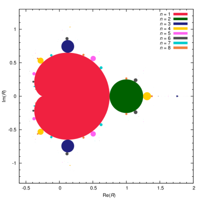
Figure 2: Stable regions of the $n$-cycles of the simplified logistic map Eq. (3) with a complex $R$; obtained from $P_{n}(R,e^{i\phi})=0$ with $\phi\in[0,2\pi]$ cf. Fig. 3 in stephenson .

Theorem 3 is not always necessary. For $n\geq 4$, $P_{n}(R,\lambda)$ is readily recognized as the factor of $A_{n}(R,\lambda)$ with the highest degree in $R$, see Table 2 and Section II.9. It can be, however, problematic, if $P_{n}(R,\lambda)$ is solved for $\lambda=1$ instead of a general $\lambda$, for $P_{n}(R,1)$ itself can be further factorized, see Table 4. Due to the technical nature of the derivation and subsequent discussions, the reader may wish to skip the rest of Section II on first reading.

II.7 Counting cycles

To show Theorem 3, we first find the degrees in $\lambda$ of $A_{n}(R,\lambda)$ (Theorem 4) and $P_{n}(R,\lambda)$ (Theorem 40). By comparing the degrees, we then show that each $P_{d}(R,\lambda)$ with ($d|n$), after some transformation, contributes one polynomial factor to $A_{n}(R,\lambda)$ (Theorem 6), and the inversion of the relation yields Theorem 3.

II.7.1 Number of the square-free cyclic polynomials

To count the square-free cyclic polynomials, we establish a one-to-one mapping between the square-free cyclic polynomials and the binary necklaces (defined below). The task is then to count the latter.

A binary necklace is a nonequivalent binary $0$-$1$ string. Two strings are equivalent if they differ only by a circular shift. For example, for $n=3$, there are $2^{3}=8$ binary strings, but only four necklaces: 000, 001, 011 and 111, since 010 and 100 are equivalent to 001, so are 110 and 101 to 011. The period of a necklace, or a binary string, is the length of the shortest non-repeating sub-sequence, e.g., the periods of $1111$, $0101$ and $0001$ are 1, 2, and 4, respectively. Obviously, the period $m$ divides $n$; and a period-$m$ necklace encompasses $m$ binary strings differed by circular shifts, e.g., $0101$ represents both $0101$ and $1010$.

Table 5: Two ways of counting the $N(4)=6$ necklaces for $n=4$.

	$m=1$		$m=2$	$m=4$	$2^{d}$	$\phi(n/d)$	$\phi(n/d)2^{d}$
$d=1$	$\mathbf{0}_{\times 4}$	$\mathbf{1}_{\times 4}$			$2=2$	$2$	4
$d=2$	$\mathbf{00}_{\times 2}$	$\mathbf{11}_{\times 2}$	$\mathbf{10}_{\times 2}(01_{\times 2})$		$2+2=4$	$1$	4
$d=4$				$\mathbf{1000}(0100,0010,0001)$	$2+2+12$
	$\mathbf{0000}$	$\mathbf{1111}$	$\mathbf{1010}(0101)$	$\mathbf{1100}(1001,0110,0011)$	$=16$	$1$	16
				$\mathbf{1110}(1101,1011,0111)$
$m\sum_{m|d,d|n}\phi(\frac{n}{d})$	$1\cdot(2+1+1)=4$		$2\cdot(1+1)=4$	$4\cdot 1=4$			$\downarrow$
$N(n)\cdot n$	$2\cdot 4$		$1\cdot 4$	$3\cdot 4$	$\rightarrow$		$6\cdot 4=24$
Bold strings are necklaces; others are their cyclic versions.
The subscript of a binary string means the number of repeats; e.g., $\mathbf{0}_{\times 4}$ means $\mathbf{0}$ repeated four times, or $\mathbf{0000}$; $\mathbf{10}_{\times 2}$ means $\mathbf{10}$ repeated twice, or $\mathbf{1010}$, etc.

To compute the number of the binary necklaces $N(n)$, we construct a sum for the length-$n$ binary strings and count it in two ways. Table 5 shows the example for the $n=4$ case. For each divisor $d$ of $n$, we collect all length-$n$ binary strings whose periods $m$ divide $d$. The total is $2^{d}$, for we have enumerated all binary strings whose periods divide $d$. We then weight them by the Euler’s totient function $\phi(n/d)$. Here, $\phi(m)$ gives the number of integers from 1 to $m$ that are coprime to $m$, e.g., $\phi(1)=1$, $\phi(3)=2$ for 1 and 2, $\phi(6)=2$ for 1 and 5. We repeat the process over other divisors $d$ of $n$, and the resulting sum is $\sum_{d|n}\phi(n/d)2^{d}$. The process for a fixed $d$ is exemplified by a row in Table 5.

We can count the above sum in another way. We recall that a period-$m$ necklace always contributes $m$ strings in the above process for a fixed $d$, and it does so for all multiples $d$ of $m$. So the total weighted contribution by this necklace is

$$m\sum_{m|d,d|n}\phi(n/d)=m\sum_{\frac{n}{d}|\frac{n}{m}}\phi(n/d)=m\,\frac{n}{m}=n,$$ (38)

where we have used the identity $\sum_{d^{\prime}|m^{\prime}}\phi(d^{\prime})=m^{\prime}$, with $d^{\prime}=n/d$ and $m^{\prime}=n/m$. Summing over the necklaces yields $N(n)\,n$. Thus, $N(n)=(1/n)\sum_{d|n}\phi(n/d)2^{d}$. The process for a fixed necklace is exemplified by a column in Table 5.

Back to our problem, there is a correspondence between the binary necklaces and the square-free cyclic polynomials. For a square-free cyclic polynomial, we construct a binary string according to its generator: if it contains $x_{k}$, the $k$th character from the left is 1, otherwise 0. The resulting string corresponds to a unique necklace; the alternative generators give the circularly-shifted binary strings. The mapping is reversible, or one-to-one. For example, if $n=3$, the square-free polynomials for $000$, $100$, $110$ and $111$ are $C_{0}=1$ (generator: 1), $C_{1}=x_{1}+x_{2}+x_{3}$ (generator: $x_{1}$), $C_{12}=x_{1}x_{2}+x_{2}x_{3}+x_{3}x_{1}$ (generator: $x_{1}x_{2}$) and $C_{123}=x_{1}x_{2}x_{3}$ (generator: $x_{1}x_{2}x_{3}$), respectively. Table 1 shows a few more examples. Thus,

Theorem 4.

The number $N_{\mathcal{B}}(n)$ of the square-free cyclic polynomials $C_{p}(\mathbf{x})$ ($p\in\mathcal{B}$) formed by $\mathbf{x}=\{x_{1},\ldots,x_{n}\}$ is

$$N_{\mathcal{B}}(n)=N(n)=(1/n)\sum_{d|n}\phi(n/d)2^{\,d},$$ (39)

which is also equal to $\deg_{\lambda}A_{n}(R,\lambda)$.

$N(n)$ = 2, 3, 4, 6, 8, 14, 20, 36, 60, 108, 188, 352, 632, …, starting from $n=1$.

II.7.2 Number of the $n$-cycles

Theorem 5.

The degree in $\lambda$ of the minimal polynomial $P_{n}(R,\lambda)$ of all $n$-cycles is equal to the number of the $n$-cycles, and is given by

$$\deg_{\lambda}P_{n}(R,\lambda)=L(n)=(1/n)\sum_{d|n}\mu(n/d)2^{\,d}.$$ (40)

Proof.

Except a few special values of $R$, the iterated map $f^{n}$ generally has $2^{n}$ distinct complex fixed points, for otherwise $f^{n}(x)-x$ would have a repeated zero at any $R$, but at $R=0$, $-x^{2^{n}}-x$ has no repeated root; a contradiction.

Each fixed point can be assigned to a point in a $d$-cycle, with $d$ being a divisor of $n$. The assignment is both complete (for a $d$-cycle point must also be a fixed point of $f^{n}$) and non-redundant (for there is no repeated fixed point of $f^{n}$). Since each of the $L(d)$ $d$-cycles contributes $d$ fixed points, we have $2^{n}=\sum_{d\,|\,n}L(d)\,d$. The Möbius inversion yields $L(n)=(1/n)\sum_{d\,|\,n}\mu(n/d)2^{\,d}$. This formula was known to several authors hao ; lutzky .

We now define $\lambda_{c}$ as the value of $\Lambda(\mathbf{x})$, evaluated at the cycle points $\mathbf{x}^{(c)}\equiv\{{x_{1}}^{(c)},\ldots,{x_{n}}^{(c)}\}$ of cycle $c$. Of course, $\lambda_{c}$ is a function of $R$. If we assume that $\lambda_{c}$ are distinct (see Remark 1 below), then the minimal polynomial $P_{n}(R,\lambda)$, as a polynomial of $\lambda$, takes the form of $\prod_{c}(\lambda-\lambda_{c})$. Thus, the degree of $P_{n}(R,\lambda)$ in $\lambda$ must be the same as the number of the $n$-cycles. ∎

Remark 1. Although all trajectory points $\mathbf{x}^{(c)}$ are distinct in different cycles, the value $\lambda_{c}$ of the polynomial $\Lambda(\mathbf{x}^{(c)})$ may happen to be the same. In this case, we shall find another cyclic polynomial $Y(\mathbf{x})$ that has different values in the two cycles [$Y(\mathbf{x})$ exists for otherwise $\mathbf{x}$ are the same in the two cycles], use $\Lambda^{\prime}(\mathbf{x})=\Lambda(\mathbf{x})+\epsilon Y(\mathbf{x})$ to list Eqs. (5), then take the limit $\epsilon\rightarrow 0$.

Remark 2. $L(n)$ is also the number of aperiodic (i.e., period equal to $n$) necklaces of length $n$, e.g., for $n=4$, out of the six necklaces, $0001$, $0011$, and $0111$ are aperiodic; but $0000$, $1111$, and $0101$ are periodic. Since a period-$d$ ($d|n$) necklace is just an aperiodic one of length-$d$ repeated $n/d$ times, and each contributes $d$ binary strings, we can count the $2^{n}$ binary strings of length $n$ as $2^{n}=\sum_{d|n}L(d)\,d$. The Möbius inversion leads to the same result of Eq. (40).

$L(n)$ = 2, 1, 2, 3, 6, 9, 18, 30, 56, 99, 186, 335, 630, …, starting from $n=1$.

Since the period $d$ of a length-$n$ necklace always divides $n$, we have

$$N(n)=\sum_{d|n}L(d).$$ (41)

We can also show this by explicit computation:

$$\sum_{d|n}L(d) =\sum_{d|n}(1/d)\sum_{c|d}\mu(d/c)2^{\,c}=(1/n)\sum_{c|n}2^{\,c}\sum_{d^{\prime}|(n/c)}\mu\left(\frac{n/c}{d^{\prime}}\right)d^{\prime}$$

$$=(1/n)\sum_{c\,|\,n}2^{\,c}\,\phi(n/c)=N(n),$$

where we have used $\phi(m)=\sum_{d^{\prime}|m}\mu(\frac{m}{d^{\prime}})\,d^{\prime}$, which is the inversion of $m=\sum_{d^{\prime}|m}\phi(d^{\prime})$, and Eq. (39). We will use Eq. (41) in proving the next theorem.

II.7.3 Relation between $P_{n}(R,\lambda)$ and $A_{n}(R,\lambda)$

Theorem 6.

The minimal polynomials $P_{d}(R,\lambda)$ of all $d$-cycles of periods $d|n$ and $A_{n}(R,\lambda)$ [defined in Eq. (7)] are related by

$$A_{n}(R,\lambda)=\prod_{cd=n}Q_{d,c}(R,\lambda),$$ (42)

where $Q_{d,c}(R,\lambda)=\prod_{k=1}^{c}P_{d}(R,e^{2k\pi i/c}\lambda^{1/c})$ is a polynomial of degree $L(d)$ in $\lambda$ representing contributions from $d$-cycles.

Proof.

Since $A_{n}(R,\lambda)$ represent all $d$-cycles with $d|n$, and each cycle holds a distinct $\lambda$, $\deg_{\lambda}A_{n}(R,\lambda)$ is at least $\sum_{d|n}L(d)$ according to Eq. (40), which is equal to $N(n)$ by Eq. (41). Since $\deg_{\lambda}A_{n}(R,\lambda)=N(n)$ by Eq. (39), each $n$-cycle occurs exactly once in $A_{n}(R,\lambda)$.

In a $d$-cycle, we have $\Lambda(\{x_{1},\ldots,x_{n}\})=(-2)^{n}x_{1}\dots x_{n}={\Lambda_{d}}^{c}$, where $\Lambda_{d}(\{x_{1},\ldots,x_{d}\})\equiv(-2)^{d}x_{1}\dots x_{d}$ and $c\equiv n/d$. So the $d$-cycle satisfies a polynomial $P_{d}(R,\lambda^{1/c})=0$, where $\lambda=\Lambda(\{x_{1},\ldots,x_{n}\})$. This is, however, not a polynomial equation, and the radical $\lambda^{1/c}$ can be removed by the product $Q_{d,c}(R,\lambda)\equiv\prod_{k=1}^{c}P_{d}(R,e^{2k\pi i/c}\,\lambda^{1/c})=0$. Now $Q_{d,c}(R,\lambda)$ is a polynomial of $\lambda$ for it is invariant under $\lambda\rightarrow e^{2\pi i}\lambda$, and thus free from radicals of the form $\lambda^{l/c}$ [if $(l,c)\neq c$]. And since $\deg_{\lambda}Q_{d,c}(R,\lambda)=\deg_{\lambda}P_{d}(R,\lambda)=L(d)$, it is also a polynomial of the lowest possible degree in $\lambda$.

Therefore, the product $\prod_{cd=n}Q_{d,c}(R,\lambda)$ can differ from $A_{n}(R,\lambda)$ only by a multiple. Since $Q_{n,1}(R,\lambda)=P_{n}(R,\lambda)$, and the coefficient of highest power of $\lambda$ is always unity in $A_{n}(R,\lambda)$ [see the definition Eq. (7)], we know by induction that the coefficients of the highest power of $\lambda$ in all $P_{n}(R,\lambda)$ and $Q_{d,c}(R,\lambda)$ are also unities. So the multiple is one, hence Eq. (42). ∎

We can now prove Theorem 3 as a corollary of Theorem 6,

$$B_{n,m}(R,\lambda) =\prod_{l=1}^{m}A_{n}(R,e^{2l\pi i/m}\lambda^{1/m})$$

$$=\prod_{c|n}\prod_{l=1}^{m}\prod_{k=1}^{c}P_{n/c}(R,e^{2k\pi i/c+2l\pi i/(mc)}\lambda^{1/(mc)})$$

$$=\prod_{c|n}\prod_{k^{\prime}=1}^{mc}P_{n/c}(R,e^{2k^{\prime}\pi i/(mc)}\lambda^{1/(mc)})=\prod_{c|n}Q_{n/c,mc}(R,\lambda).$$

Taking the logarithm (formally) yields $\log B_{n,m}=\sum_{d|n}\log Q_{d,mn/d}$, where $d=n/c$. The inversion is $\log Q_{n,m}=\sum_{d|n}\mu(n/d)\log B_{d,mn/d}$, or

$$Q_{n,m}(R,\lambda)=\prod_{d|n}B_{d,mn/d}(R,\lambda)^{\mu(n/d)}, \ref{eq:primfac}^{\prime}$$ ()

which is reduced to Eq. (37) with $m=1$ for $Q_{n,1}(R,\lambda)=P_{n}(R,\lambda)$.

II.8 Intersection of cycles and further factorization at the onset point

Table 4 shows that the onset polynomial $P_{n}(R,\lambda=1)$ for the $n$-cycles can be further factorized. This is because the intersection of an $n$-cycle and a shorter $d$-cycle ($d|n$, $d<n$) forces the two to share orbits (this cannot happen if $d\centernot|n$, for the orbits would be out of phase). Consequently, upon the intersection, $P_{n}(R,\lambda)$ from the $n$-cycle has to accommodate $P_{d}(R,\lambda^{\prime})$ from the $d$-cycle, with $\lambda^{\prime}$ being a primitive $(n/d)\,$th root of $\lambda$.

At the intersection, the shorter $d$-cycle is branched or “bifurcated” by $(n/d)$-fold to the $n$-cycle. The simplest example is the first bifurcation point at $R=3/4$ for $d=1,n=2$, where the fixed point Eq. (7-1) bifurcates to the 2-cycle Eq. (7-2). The second bifurcation point at $R=5/4$ for $d=2,n=4$ is similar, cf. Section II.5.

We will show below that such branching generally can only happen at the onset of the $n$-cycle, where $\lambda=1$. Further, with a real $R$, only a two-fold branching is possible, but a complex $R$ allows higher-fold branchings.

If an $n$-cycle is not born out of the above branching, we call it an original cycle, e.g., the 4-cycle at $R_{a}^{\prime}=5/4$ is born out of bifurcation, see Fig. 1(d), but the other at $R_{a}=(3+\sqrt[3]{108})/4$ is original, see Fig. 1(e), also the discussion after Eq. (7-4). Both types of cycles exist in $P_{n}(R,\lambda=+1)$, as separate factors; and the factor responsible for the original cycles, or the original factor below, is given by the following formula.

Theorem 7.

The original factor $S_{n}(R)$ of $P_{n}(R,\lambda)$ at the onset is given by

$$S_{n}(R)=\frac{P_{n}(R,1)}{\prod_{cd=n,\;c>1}\left[\,\prod_{(k,c)=1}P_{d}\left(R,e^{2k\pi i/c}\right)\right]},$$ (43)

where the inner product on the denominator is carried over $k$ from 1 to $c$ that are coprime to $c$.

We illustrate Theorem 7 through a few examples before giving a proof. For $n=1$, $S_{1}(R)=P_{1}(R,1)=-4R-1$ as the denominator is unity.

For $n=2$, $P_{2}(R,1)=4R-3$. But $P_{1}(R,-1)=-4R+3$. So $S_{2}(R)=P_{2}(R,1)/P_{1}(R,-1)=-1$. This means that there is no original 2-cycle and the only 2-cycle comes from period doubling.

For $n=3$, $P_{3}(R,1)=-(4R-7)(16R^{2}-4R+7)$, whose second factor is equal to $\big{(}-4R+\frac{1-3\sqrt{3}i}{2}\big{)}\big{(}-4R+\frac{1+3\sqrt{3}i}{2}\big{)}=\prod_{k=1,2}P_{1}(R,e^{2k\pi i/3})$. Thus $S_{3}(R)=-4R+7$.

For $n=4$, $P_{4}(R,1)=(4R-5)(16R^{2}+8R+5)\bigl{[}(4R-3)^{3}-108\bigr{]}$. But $P_{2}(R,-1)=4R-5$ (for $c=2$) and $\prod_{k=1,3}P_{1}(R,e^{k\pi i/2})=(-4R-2i-1)(-4R+2i-1)=16R^{2}+8R+5$ (for $c=4$). Dividing $P_{4}(R,1)$ by the two factors yields $S_{4}(R)=(4R-3)^{3}-108$, whose only real root $R=(3+\sqrt[3]{108})/4$ corresponds to the onset of the original cycle. Note $R=5/4$ is excluded from $S_{4}(R)$ as it comes from period-doubling the 2-cycle.

We now prove Theorem 7. Suppose $n=c\,d$, we have, from Eq. (3),

$$x_{l+1}-x_{d+l+1}=-(x_{l}+x_{d+l})(x_{l}-x_{d+l}).$$

We apply the equation to $l=1,\ldots,m$, and the product is

$$x_{m+1}-x_{m+d+1}=(-1)^{m}\left[\,\prod_{l=1}^{m}(x_{l}+x_{d+l})\right](x_{1}-x_{d+1}).$$

We now set $m$ to $0,d,\ldots,(c-1)\,d$ in this equation, add them together, eliminate $x_{1}-x_{d+1}$ (which is nonzero in a cycle), and

$$\sum_{c^{\prime}=0}^{c-1}(-1)^{c^{\prime}d}\prod_{l=1}^{c^{\prime}d}(x_{l}+x_{d+l})=0.$$ (44)

Note Eq. (44) holds for every divisor $c$ of $n$ ($c>1$). We now have

Theorem 8.

An $n$-cycle and a shorter $d$-cycle ($d|n$, $d<n$) intersect only at the onset of the $n$-cycle, and $\prod_{k=1}^{d}f^{\prime}(x_{k})=(-2)^{d}x_{1}\dots x_{d}$ is a primitive $(n/d)$th root of unity there.

Proof.

At the intersection of the $n$- and $d$-cycles, $x_{l}$ repeats itself after $d$ steps, so $x_{d+l}=x_{l}$; and Eq. (44) becomes,

$$1+q+\dots+q^{c-1}=0,$$ (45)

where $q=(-2)^{d}\,x_{1}\dots x_{d}$. Multiplying Eq. (45) by $q-1$ yields $1=q^{c}=(-2)^{n}\,x_{1}\dots x_{n}$. So the $n$-cycle is at its onset.

Further $q$ is a primitive $c$th root of unity. Suppose the contrary: $q=e^{2k\pi i/c}$ and $(k,c)=g>1$, then by $c_{1}\equiv c/g$, $k_{1}\equiv k/g$, we have

$$q=e^{2k_{1}\pi i/c_{1}}.$$ (46)

Similar to Eq. (45), we can apply Eq. (44) with $c\rightarrow g$ and $d\rightarrow dc_{1}$, and

$$1+q_{1}+\dots+{q_{1}}^{g-1}=0,$$

where $q_{1}=(-2)^{dc_{1}}\,x_{1}\dots x_{dc_{1}}=q^{c_{1}}$. But by Eq. (46), $q^{c_{1}}=e^{2k_{1}\pi i}=1$, and $1+q_{1}+\dots+{q_{1}}^{g-1}=g>0$; a contradiction. ∎

Remark 1. The only real $q$ is $q=-1$ for $c=2$, i.e., a period-doubling. On the complex domain, however, we can have a $c$-fold branching with $c>2$, which corresponds to a contact points between “bulbs” in the Mandelbrot set, see Fig. 2.

By Theorem 8, $P_{n}(R,\lambda)$ at the onset point includes $P_{d}(R,e^{2k\pi i/c}\lambda^{1/c})$ for every possible combination of $k$ and $c$, such that $(k,c)=1$, $c|n$, and $c>1$. Dividing the factors from $P_{n}(R,\lambda)$ yields Theorem 7.

II.9 Degrees in $R$

Theorem 9.

The degrees in $R$ of $A_{n}(R,\lambda)$, $P_{n}(R,\lambda)$ and $S_{n}(R)$ are

$$\deg_{R}A_{n}(R,\lambda) =\sum_{d|n}\phi(n/d)2^{d-1},$$ (47a)

$$\deg_{R}P_{n}(R,\lambda) =\sum_{d|n}\mu(n/d)2^{d-1}\equiv\beta(n),$$ (47b)

$$\deg S_{n}(R) =\beta(n)-\sum_{d|n,d<n}\beta(d)\,\phi(n/d).$$ (47c)

Proof.

We first prove Eq. (47a). We recall the subscript $p$ of $C_{p}$ denotes a sequence of indices $k$ in the generating monomial $\prod_{k}{x_{k}}^{e_{k}}$. But for a square-free cyclic polynomial, each $k$ occurs no more than once, so $p$ also represents a set of indices, e.g., $p=1$ represents $\{1\}$, ($C_{1}=x_{1}+\dots+x_{n}$, generator: $x_{1}$) and $p=13$ represents $\{1,3\}$ ($C_{13}=x_{1}\,x_{3}+x_{2}\,x_{4}+\dots+x_{n}\,x_{2}$, generator: $x_{1}\,x_{3}$, assuming $n\geq 4$); more examples are listed in Table 1). In this proof, we shall also use $p$ to denote the corresponding index set, $|p|$ the set size, i.e., the number of indices in the set, and $\bar{p}\equiv\{1,\ldots,n\}\backslash p$ the complementary set. Obviously, $|\bar{p}|+|p|=n$. Further, we will include $p$ that correspond to alternative generators of the same cyclic polynomial, e.g., we allow $p=\{2\}$, $\{3\}$, …, $\{n\}$, although they represent the same cyclic polynomial $C_{1}$ as $p=\{1\}$.

Next, we recall the matrix elements $T_{pq}(R)$ arise from the square-free reduction of $\Lambda(\mathbf{x})C_{p}(\mathbf{x})=(-2)^{n}x_{1}\dots x_{n}\,C_{p}(\mathbf{x})$. A single replacement ${x_{k}}^{2}\rightarrow R-x_{k+1}$ produces two new terms: in the first, ${x_{k}}^{2}\rightarrow R$, and in the second, ${x_{k}}^{2}\rightarrow-x_{k+1}$. We call the two type 1 and type 2 replacements, respectively. If a monomial term $t(R,\mathbf{x})$ results from $l_{1}$ type 1 and $l_{2}$ type 2 replacements during the reduction of a term $s(\mathbf{x})$ in $\Lambda(\mathbf{x})C_{p}(\mathbf{x})$, then the degrees in $\mathbf{x}$, for any $x_{k}$, of $s(\mathbf{x})$ and $t(R,\mathbf{x})$ are related as

$$\deg_{\mathbf{x}}s(\mathbf{x})-\deg_{\mathbf{x}}t(R,\mathbf{x})=2l_{1}+l_{2}.$$ (48)

Similarly, the degrees in $R$ satisfy

$$\deg_{R}s(\mathbf{x})-\deg_{R}t(R,\mathbf{x})=-l_{1},$$

but since $\deg_{R}s(\mathbf{x})=0$,

$$\deg_{R}t(R,\mathbf{x})=l_{1}.$$ (49)

Now if the monomial $t(R,\mathbf{x})$ settles in the $q$th column of the matrix $\mathbf{T}(R)$, as part of $T_{pq}(R)C_{q}(\mathbf{x})$ in Eq. (5), then $t(R,\mathbf{x})$ must be a generator of $C_{q}(\mathbf{x})$; so

$$\deg_{\mathbf{x}}t(R,\mathbf{x})=|q|.$$ (50)

Since $s(\mathbf{x})$ is part of $\Lambda(\mathbf{x})C_{p}(\mathbf{x})$, we have

$$\deg_{\mathbf{x}}s(\mathbf{x})=\deg_{\mathbf{x}}\Lambda(\mathbf{x})+\deg_{\mathbf{x}}C_{p}(\mathbf{x})=n+|p|.$$ (51)

From Eqs. (48), (50), (51), we get

$$n+|p|-|q|=2\,l_{1}+l_{2},$$

and

$$l_{1}=(n+|p|-|q|-l_{2})/2\leq(n+|p|-|q|)/2.$$ (52)

By Eq. (49), we get

$$\deg_{R}T_{pq}(R)=\max\{\deg_{R}t(R,\mathbf{x})\}=\max\{l_{1}\}\leq(n+|p|-|q|)/2,$$

where the equality holds when all replacements are type 1 ($l_{2}=0$).

Finally, each term of the determinant $A_{n}(R,\lambda)=\big{|}\lambda\,\mathbf{I}-\mathbf{T}(R)\big{|}$ is given by $(-1)^{s}\prod_{p}\big{[}\lambda\,\delta_{pq}-T_{pq}(R)\big{]}$, where $p$ runs through rows of the matrix and $\{q\}$ is a permutation of $\{p\}$, with $(-1)^{s}$ being the proper sign. Summing over rows under this condition yields

$$\deg_{R}A_{n}(R,\lambda)=\max\sum_{p\in\mathcal{B}}\deg T_{pq}(R)\leq N(n)\,\big{(}n+|p|-|q|\big{)}/2=nN(n)/2,$$

where equality can be achieved if $q=\bar{p}$ in every row. By Eq. (39) we have Eq. (47a). The first few values are 1, 3, 6, 12, 20, 42, 70, 144, 270, 540, 1034, 2112, 4108, …, starting from $n=1$.

To show Eq. (47b), we take the degree in $R$ of Eq. (42). So $\sum_{d|n}\beta(d)\,\big{(}n/d\big{)}=N(n)\,n/2$, whose inversion is $\beta(n)/n=\sum_{d|n}\mu(n/d)\,N(d)/2=L(n)/2$. The last step follows from inverting Eq. (41). The first few values are 1, 1, 3, 6, 15, 27, 63, 120, 252, 495, 1023, 2010, 4095, …, starting from $n=1$.

Eq. (47c) follows directly from taking the degree in $R$ of Eq. (43). The first few values are 1, 0, 1, 3, 11, 20, 57, 108, 240, 472, 1013, 1959, 4083, …, starting from $n=1$. ∎

Eqs. (47b) was long known mira , and (47c) was recently derived blackhurst .

III Hénon map

We now extend the method to the Hénon map henon :

$$x_{k+1}=1+y_{k}-a\,{x_{k}}^{2},\quad y_{k+1}=b\,x_{k}.$$ (53)

We change variable $x_{k}\leftarrow ax_{k}$, $y_{k}\leftarrow ay_{k}$, and

$$x_{k+1}=a+y_{k}-{x_{k}}^{2},\quad y_{k+1}=b\,x_{k}. \ref{eq:henon}^{\prime}$$ ()

Since neither $a$ nor $b$ is changed during the transformation, Eq. (53) and Eq. ($\ref{eq:henon}^{\prime}$) share the same onset and bifurcation points in terms of $a$ and $b$. We also see that if $b\rightarrow 0$ and $a\rightarrow R$, Eq. ($\ref{eq:henon}^{\prime}$) is reduced to the logistic map Eq. (3).

Since $y_{k}=b\,x_{k-1}$, we can ignore $y_{k}$ and work with cyclic polynomials of $x_{k}$ only, the square free reduction is now ${x_{k}}^{2}\rightarrow a+bx_{k-1}-x_{k+1}$.

The stability of Eq. ($\ref{eq:henon}^{\prime}$) can be found from the Jacobian matrix

$$J_{b}(x_{k})\equiv\left(\begin{array}[]{ccc}\partial x_{k+1}/\partial x_{k}&\partial x_{k+1}/\partial y_{k}\\ \partial y_{k+1}/\partial x_{k}&\partial y_{k+1}/\partial y_{k}\\ \end{array}\right)=\left(\begin{array}[]{ccc}-2x_{k}&1\\ b&0\end{array}\right).$$

The eigenvalue $\lambda$ of the composite Jacobian $J_{b}(x_{1})\cdots J_{b}(x_{n})$ can be computed from

$$\big{|}\,\lambda\,\mathbf{I}-J_{b}(x_{1})\cdots J_{b}(x_{n})\,\big{|}=\lambda^{2}-\Theta(\mathbf{x})\,\lambda+(-b)^{n}=0,$$ (54)

where $\Theta(\mathbf{x})$ and $(-b)^{n}$ are the trace and determinant of the matrix product $J_{b}(x_{1})\cdots J_{b}(x_{n})$, respectively hitzl . In a stable cycle, the magnitude of $\lambda$ cannot exceed 1; so we replace $\lambda$ by $+1$ or $-1$ in Eq. (54) to obtain the onset or bifurcation point, respectively. Eq. (54) is the counterpart of Eq. (2).

Since cyclically rotating matrices in a product does not alter the trace, $\Theta(\mathbf{x})$ is a cyclic polynomial of $\mathbf{x}=\{x_{k}\}$. Thus, we can use $\Theta(\mathbf{x})$ to list Eqs. (6) and then replace $\Theta(\mathbf{x})$ by $\lambda+(-b)^{n}/\lambda$ or $\pm\big{[}1+(-b)^{n}\big{]}$ in Eq. (7) to complete the solution.

Table 6: Onset and bifurcation polynomials of the $n$-cycles of the Hénon map.

$n$	$\Theta(\mathbf{x})$	Onset $P_{n}(a,b,+1)$ †,‡	Bifurcation $P_{n}(a,b,-1)$ †,‡
1	$-2x_{1}$	$-A-(b-1)^{2}$	$-A+3(b-1)^{2}$
2	$4C_{12}+2b$	$A-3(b-1)^{2}$	$A-B^{(2)}_{5,-6}$
3	$-8C_{123}-2bC_{1}$	$\left(-A+B^{(2)}_{7,10}\right)$ $\left\{\left[A-\frac{1}{2}B^{(2)}_{1,-8}\right]^{2}+\frac{27}{4}(b^{2}-1)^{2}\right\}$	$\begin{aligned} -A^{3}&+2B^{(2)}_{4,1}A^{2}-9B^{(4)}_{2,-6,-7}A\\ &+9B^{(6)}_{9,6,2,-10}\end{aligned}$
4	$16C_{1234}+4bC_{12}+2b^{2}$	$\left(A-B^{(2)}_{5,-6}\right)$ $\left\{\left[A+(b+1)^{2}\right]^{2}+4(b^{2}-1)^{2}\right\}$ $\left\{\left[A-3(b+1)^{2}\right]^{3}-108(b-1)^{2}(b+1)^{4}\right\}$	$\begin{aligned} &A^{6}-4A^{5}B^{(2)}_{3,2}+A^{4}B^{(4)}_{47,68,38}\\ &-3A^{3}B^{(6)}_{47,62,-83,-212}+\left({B^{(4)}_{17,12,-6}}\right)^{3}\\ &+A^{2}B^{(4)}_{17,12,-6}B^{(4)}_{31,-60,-186}\end{aligned}$
5	$\begin{aligned} -&32C_{12345}\\ -&8bC_{123}-2b^{2}C_{1}\end{aligned}$	$\begin{aligned} &-\Big{(}A^{4}-B^{(2)}_{1,-12}A^{3}+B^{(4)}_{1,6,21}A^{2}\\ &+B^{(6)}_{9,-14,70,-80}A+B^{(4)}_{1,1,1}B^{(4)}_{31,-89,121}\Big{)}\\ &\Big{(}A^{11}-B^{(2)}_{31,14}A^{10}+2B^{(4)}_{208,206,377}A^{9}\\ &-\cdots-75728722b-28629151\Big{)}\end{aligned}$	$\begin{aligned} -A^{15}&+2B^{(2)}_{16,1}A^{14}-B^{(4)}_{448,60,669}A^{13}\\ &+\cdots+1291467969\end{aligned}$
⋮	⋮	⋮	⋮
9	$\begin{aligned} &-512C_{1\dots 9}\\ &-\cdots-2b^{4}C_{1}\end{aligned}$	$\begin{aligned} &-(A^{6}+12bA^{5}+\dots)\big{(}A^{6}-4B^{(2)}_{4,1}A^{5}+\dots\big{)}\\ &\Big{(}A^{240}-8B^{(2)}_{61,1}A^{239}+4B^{(4)}_{29525,1019,58188}A^{238}\\ &-\dots+120670698649\dots 712084645033\Big{)}\end{aligned}$	$\begin{aligned} &-\big{(}A^{252}-504(1+b^{2})A^{251}\\ +&4B^{(4)}_{31500,16,62067}A^{250}-\dots\\ +&5842146539\dots 9260477441\big{)}\end{aligned}$
† Definitions: $A\equiv 4a$, $B^{(2)}_{p,q}\equiv p(b^{2}+1)+qb$, $B^{(4)}_{p,q,r}\equiv p(b^{4}+1)+q(b^{3}+b)+rb^{2}$, $B^{(6)}_{p,q,r,s}\equiv p(b^{6}+1)+q(b^{5}+b)+r(b^{4}+b^{2})+sb^{3}$, $\dots$.
‡ The onset polynomials for $n$ from 1 to 4, and the bifurcation polynomials for $n$ from 1 to 3, agree with those in ref. hitzl .

We computed the polynomials of $a$ and $b$ at the onset and bifurcation points for $n$ up to 9. The polynomials of $a$ and $b$ at the onset and bifurcation points, as well as $\Theta(\mathbf{x})$, are listed in Table 6 for small $n$ (for larger $n$, see the website in Section V).

IV Cubic map

We now study the following cubic map strogatz

$$x_{k+1}=f(x_{k})=r\,x_{k}-{x_{k}}^{3}.$$ (55)

Since the new replacement rule

$${x_{k}}^{3}\rightarrow r\,x_{k}-x_{k+1}$$ (56)

no longer eliminates squares, we must extend the basis set of cyclic polynomials from the square-free ones to the cube-free ones, in using Eq. (6). We include in the basis of expansion $C_{112}={x_{1}}^{2}x_{2}+{x_{2}}^{2}x_{3}+\dots+{x_{n}}^{2}x_{1}$ ($n\geq 3$), but not $C_{1112}={x_{1}}^{3}x_{2}+{x_{2}}^{3}x_{3}+\dots+{x_{n}}^{3}x_{1}$.

However, we only need the cube-free cyclic polynomials of even degrees in $\mathbf{x}$ to solve the problem, because Eq. (55) contains only linear and cubic terms, a cyclic polynomial with an odd (even) degree in $\mathbf{x}$ can never be reduced to one with an even (odd) degree by Eq. (56). For technical reasons, we will not use polynomials of odd degrees, because the map allows a symmetric $2n$-cycle: $x_{1},x_{2},\ldots,x_{n},-x_{1},-x_{2},\ldots,-x_{n}$ (see Fig. 3), which makes all odd cyclic polynomials zero, e.g., $C_{1}=x_{1}+x_{2}+\dots+x_{n}-x_{1}-x_{2}-\dots-x_{n}=0$. Thus, the zero determinant condition, similar to that in Eq. (7), would be useless for these cycles, if the odd-degree polynomials were used.

Figure 3: Odd-cycles of the cubic map.

We therefore have a theorem similar to Theorem 1.

Theorem 10.

For the cubic map Eq. (55), any cyclic polynomial $K(\mathbf{x})$ of an $n$-cycle orbit $\mathbf{x}=\{x_{1},\ldots,x_{n}\}$ with an even degree in $\mathbf{x}$ is a linear combination of the even cube-free cyclic polynomials $C_{p}(\mathbf{x})$:

$$K(\mathbf{x})=\sum_{p\in\mathcal{B}}f_{p}(R)C_{p}(\mathbf{x}),$$

where $\mathcal{B}=\{0,11,12,13,\ldots,1122,1123,\ldots\}$ is the set of indices of all even cube-free cyclic polynomials, and $f_{p}(R)$ are polynomials of $R$.

With the above change, the rest derivation is similar to that of the logistic map. The new $\Lambda(\mathbf{x})$ should be $\prod_{k=1}^{n}f^{\prime}(x_{k})=\prod_{k=1}^{n}(r-3{x_{k}}^{2})$. The polynomials of $r$ at the onset and bifurcation points for some small $n$ are shown in Table 7 (general $\lambda$) and Table 8 ($\lambda=\pm 1$); for larger $n$ up to 8, we have saved the data on the website in Section V. The representative $r$ values are listed in Table 9. For complex $r$ and $\mathbf{x}$, we have plotted Fig. 4 for regions of stability.

Table 7: Minimal polynomials $P_{n}(r,\lambda)$ of the $n$-cycles of the cubic map Eq. (55).

$n$	$P_{n}(r,\;\lambda)$ †
1	$(\lambda-r)(\lambda+2r-3)$
2	$\big{[}\cancel{\lambda-(2r+3)^{2}}\big{]}(\lambda+2r^{2}-9)$
3	$\begin{aligned} &\lambda^{4}+2(r+6)(r^{2}-9)\lambda^{3}-6\big{(}8r^{6}+12r^{5}-66r^{4}-81r^{3}+54r^{2}-243r-729\big{)}\lambda^{2}+2(r^{2}-9)\big{(}16r^{7}-252r^{5}\\ -&216r^{4}+648r^{3}+972r^{2}+2187r+4374\big{)}\lambda+2r(2r-3)(2r+3)^{2}(r^{2}-9)(2r^{2}-9)^{2}(4r^{2}+9)+531441\end{aligned}$
4	$\begin{aligned} &\big{[}\cancel{(\lambda-8r^{4}+54r^{2}+81)^{2}-4(r^{2}-9)^{2}\lambda}\big{]}\,^{\ddagger}\,\big{[}\lambda^{8}+2(5r^{4}-324)\lambda^{7}+2(112r^{8}-1296r^{6}+3807r^{4}-91854)\lambda^{6}\\ +&\dots+18075490334784r^{8}-61004779879896r^{6}-411782264189298r^{4}+1853020188851841\big{]}\end{aligned}$
⋮	⋮
† The factors from odd-cycles (see Section IV.2) are struck out.
‡ The $n=4$ odd-cycles satisfy $(\lambda^{\mathrm{odd}}+9)^{2}-2(\lambda^{\mathrm{odd}}-27)r^{2}-8r^{4}=0$, where $\lambda^{\mathrm{odd}}=\pm\sqrt{\lambda}$.

Table 8: Onset and bifurcation polynomials of the $n$-cycles of the cubic map Eq. (55).

$n$	Onset $P_{n}(r,+1)$ †	Bifurcation $P_{n}(r,-1)$ †
1	$-(r-1)^{2}$	$-(r+1)(r-2)$
2	$-2(r-2)(r+1)(r+2)^{2}$	$-(r^{2}-5)(2r^{2}+6r+5)$
3	$\begin{aligned} &(r^{2}+r+1)(4r^{2}-14r+13)\\ &(4r^{8}+16r^{7}-35r^{6}-206r^{5}-113r^{4}\\ &+376r^{3}+715r^{2}+1690r+2197)\end{aligned}$	$\begin{aligned} &16r^{12}+24r^{11}-288r^{10}-434r^{9}\\ +&1539r^{8}+2358r^{7}-1434r^{6}-2556r^{5}-8541r^{4}\\ -&11816r^{3}+15288r^{2}+24696r+38416\end{aligned}$
4	$\begin{aligned} -&8(r^{2}-8)(r^{2}-5)(r^{2}+1)(2r^{2}-6r+5)\\ &(2r^{2}+6r+5)(2r^{4}-13r^{2}-25)^{2}\\ &(1024r^{22}-32512r^{20}+402304r^{18}\\ -&2364832r^{16}+5389924r^{14}+9715769r^{12}\\ -&73067038r^{10}+58934785r^{8}+235761152r^{6}\\ -&160907264r^{4}-671088640r^{2}-2097152000)\end{aligned}$	$\begin{aligned} &-(16r^{8}-216r^{6}+410r^{4}+2142r^{2}+1681)\\ &(8192r^{32}-387072r^{30}+7834624r^{28}-88031232r^{26}\\ &+585876512r^{24}-2158227720r^{22}+2211361312r^{20}\\ &+15958823175r^{18}-68871388441r^{16}+59290039854r^{14}\\ &+234882618673r^{12}-524807876277r^{10}-72612143404r^{8}\\ &+308406843576r^{6}+1539579145957r^{4}-7984925229121)\end{aligned}$
⋮	⋮	⋮
8	$\begin{aligned} &-8192(r^{4}+1)(2r^{4}-18r^{2}+41)\\ &(8r^{4}-48r^{3}+108r^{2}-108r+41)\\ &(8r^{4}+48r^{3}+108r^{2}+108r+41)\dots\\ &(22016722240\dots 14954924752896r^{3108}\\ &-\dots-180097954\dots 2522413056\times 10^{400})\end{aligned}$	$\begin{aligned} -&(17592186044416r^{80}+\dots+\\ &144564714832407908402064153121600801)\\ &(4841528421712030\dots 03048551060078592r^{3200}\\ &-\dots-25263420710\dots 173884723232001)\end{aligned}$
† Although $P_{n}(r,\lambda)$ is the minimal polynomial for a general $\lambda$, it may contain a pre-factor (e.g., $-2$ in the $n=2,\lambda=+1$ case).

Table 9: Smallest positive $r$ at the onset and bifurcation points of the $n$-cycles of the cubic map.

$n^{\dagger}$	Onset‡	Bifurcation‡	#∗	$n^{\dagger}$	Onset‡	Bifurcation‡	#∗
$1$	$1.0000000000_{1}$	$2.0000000000_{1}$	2	$6$	$2.3334877526_{304}$	$2.3355337580_{336}$	56
$2^{\prime}$	$2.0000000000_{1}$	$2.2360679775_{2}$	2	$6^{\prime}$	$2.4608286739_{12}$	$2.4657090579_{336}$	4
$3$	$2.4504409645_{8}$	$2.4608286739_{12}$	4	$7$	$2.3729872678_{1080}$	$2.3732727868_{1092}$	156
$4$	$2.5478350393_{22}$	$2.5488312193_{32}$	8	$8$	$2.3525990555_{3108}$	$2.3527637793_{3200}$	400
$4^{\prime\prime}$	$2.2360679775_{2}$	$2.2880317545_{32}$	2	$8^{\prime}$	$2.5488312193_{32}$	$2.5493247379_{3200}$	8
$5$	$2.3939250274_{112}$	$2.3957922744_{120}$	24	$8^{\prime\prime\prime}$	$2.2880317545_{32}$	$2.2992279397_{3200}$	2
† $\,{}^{\prime}$, $\,{}^{\prime\prime}$, or $\,{}^{\prime\prime\prime}$ means a cycle under the first, second, or third successive period-doubling, respectively.
‡ The subscripts are the degrees of the corresponding minimal polynomial.
∗ The number of similar cycles (for $n>1$, only half of them have positive $r$).

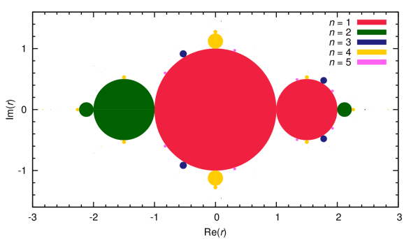
Figure 4: Stable regions of the $n$-cycles of the cubic map Eq. (55) with a complex $R$; obtained from $P_{n}(R,e^{i\phi})=0$ with $\phi\in[0,2\pi]$, cf. Fig. 2.

IV.1 Counting cycles

We now compute the number of the even cube-free cyclic polynomials by establishing a one-to-one correspondence between the cube-free cyclic polynomials and the ternary necklaces, in which each bead of the string is assigned a number 0, 1, or 2, instead of just 0 or 1. For example, the necklace $\mathbf{212001\cdots}$ corresponds to $C_{112336}(\mathbf{x})$, whose generator is ${x_{1}}^{2}\,{x_{2}}\,{x_{3}}^{2}\,x_{6}$: the first bead is 2 for ${x_{1}}^{\mathbf{2}}$, the second is 1 for ${x_{2}}^{\mathbf{1}}$, the third is 2 for ${x_{3}}^{\mathbf{2}}$, and the sixth is 1 for ${x_{6}}^{\mathbf{1}}$. A necklace is even, if the corresponding cyclic polynomial has an even degree in $\mathbf{x}$. This means that the sum of numbers (0, 1, or 2) on the beads of the necklace, which equals the degree in $\mathbf{x}$ of the polynomial, is also even.

Theorem 11.

The number of the even ternary necklaces or the cube-free cyclic polynomials for the cubic map of even degrees in $\mathbf{x}$ is given by

$$N_{e}(n)=\frac{1}{n}\sum_{cd=n}\phi(c)\left[3^{d}-\mathrm{odd}(c)\frac{3^{d}-1}{2}\right],$$ (57)

where $\mathrm{odd}(c)\equiv\big{[}1-(-1)^{c}\big{]}/2$ is 1 if $c$ is odd or 0 if even.

Proof.

We first show that the number of even ternary strings is $(3^{n}+1)/2$. Consider the generating function

$$Z\big{(}\{x_{1},x_{2},\dots,x_{n}\}\big{)}=\prod_{i=1}^{n}(1+x_{i}+{x_{i}}^{2}),$$

where $1$, $x_{i}$, and $x_{i}^{2}$ correspond to the states that bead $i$ taking the number $0$, $1$, and $2$, respectively; and the product over $n$ sums over states of independent beads. In the expansion of $Z(\mathbf{x})$, each term (which takes the form ${x_{1}}^{e_{1}}{x_{2}}^{e_{2}}\dots x_{n}^{e_{n}}$, with $e_{i}=0,1,2$) represents a unique ternary string $e_{1}e_{2}\dots e_{n}$, which is even, if $e_{1}+e_{2}+\dots+e_{n}$ is so. By setting $x_{1}=x_{2}=\dots=x_{n}=1$, $Z=3^{n}$ equals the total number of ternary strings. By setting $x_{1}=x_{2}=\dots=x_{n}=-1$, a term representing an even (odd) ternary string is $+1$ ($-1$); and $Z=(1-1+1)^{n}=1$ equals the difference between the number of even strings and that of odd strings. Thus, the average $(3^{n}+1)/2$ gives the number of even ternary strings.

Table 10: Two ways of counting the $N_{e}(2)=4$ ternary necklaces for $n=2$.

	$m=1$			$m=2$	$c=n/d$	$T(d,c)$ †	$\phi(c)$	$\phi(n/d)T(d,c)$
$d=1$	$\mathbf{0}_{\times 2}$	$\mathbf{1}_{\times 2}$	$\mathbf{2}_{\times 2}$		$2$	$3$	$1$	3
$d=2$	$\mathbf{00}$	$\mathbf{11}$	$\mathbf{22}$	$\mathbf{20}(02)$ ‡	$1$	$3+1\cdot 2=5$	$1$	5
$m\sum_{m|d,d|n}\phi(\frac{n}{d})$	$1\cdot(1+1)=2$			$2\cdot 1=2$				$\downarrow$
$N_{e}(n)\cdot n$	$3\cdot 2$			$1\cdot 2$	$\rightarrow$			$4\cdot 2=3+5$
Bold strings are necklaces; others are their cyclic versions.
The subscript of a string means the number of repeats; e.g., $\mathbf{1}_{\times 2}$ means $\mathbf{1}$ repeated twice, or $\mathbf{11}$;
† $T(d,c)\equiv 3^{d}-\mathrm{odd}(c)(3^{d}-1)/2$, which is $3^{d}$ if $c$ is even, or $(3^{d}+1)/2$ if $c$ is odd.
‡ The odd binary strings $\mathbf{10}$, $01$, $\mathbf{21}$, and $12$ do not contribute to the sum, and are excluded from $T(d,c)$.

The rest counting process is similar to that in Section II.7: we construct the sum $nN_{e}(n)$ by two ways, as exemplified in Table 10. In the first way, for a fixed $d$ ($d|n$), if $c\equiv n/d$ is even, we count all ternary strings whose period $m$ divide $d$, but if $c$ is odd, we count only ternary strings whose first $d$ beads are even (because repeating an odd string an odd number times does not yield an even string); in either case, we multiple the result by $\phi(c)$. The process for a fixed $d$ corresponds to a row of Table 10. Repeating the process for all $d$ gives $\sum_{cd=n}T(d,c)\,\phi(c)$, where $T(d,c)$ is the total number $3^{d}$ of period-$d$ ternary strings if $c$ is even, or the number $(3^{d}+1)/2$ of even strings if $c$ is odd.

In the second way, we look at the contribution from each necklace to the above sum. An even period-$m$ necklace contributes a total of $m\times\sum_{m|d,d|n}\phi(n/d)=n$ [the multiplier $m$ is for the $m$ cyclic versions, cf. Eq. (38)], while an odd necklace contributes nothing. Thus, the sum equals $N_{e}(n)\cdot n$. The process for a fixed necklace corresponds to a column of Table 10.

So

$$N_{e}(n)\cdot n=\sum_{cd=n}T(d,c)\,\phi(c),$$

which is Eq. (58) after we divide both sides by $n$. ∎

$N_{e}(n)$ = 2, 4, 6, 14, 26, 68, 158, 424, …, starting from $n=1$.

The characteristic polynomial $A_{n}(r,\lambda)$ from the determinant equation has a degree $N_{e}(n)$ in $\lambda$. Again, it encompasses the factors for the $n$-cycles and the shorter $d$-cycles, as long as $d|n$. The minimal polynomial for the $n$-cycles can be obtained by Theorem 3 with proper substitutions [$R\rightarrow r$, $A_{n}(R,\lambda)\rightarrow A_{n}(r,\lambda)$, etc.]. The degree of the polynomial is given by

Theorem 12.

The degree in $\lambda$ of the minimal polynomial $P_{n}(r,\lambda)$ of the $n$-cycles is

$$L_{e}(n)=\frac{1}{n}\sum_{cd=n}\mu(c)\left[1+\mathrm{odd}(c)\frac{3^{d}-1}{2}\right],$$ (58)

where $\mathrm{odd}(n)=[1-(-1)^{n}]/2$ is $1$ for an odd $n$, but $0$ for an even $n$.

Eq. (58) follows from the inversion $L_{e}(n)=\sum_{d|n}\mu(n/d)\,N_{e}(n)$, after some algebra, as shown in Appendix B. $L_{e}(n)$ = 2, 2, 4, 10, 24, 60, 156, 410, …, starting from $n=1$. This is also the number of the $n$-cycles hao . Note that, for $n>1$, half of the cycles have negative $r$, and the $x_{k}$ are imaginary. However, in a transformed map,

$$z_{k+1}=r\,z_{k}\,(1-{z_{k}}^{2}),$$

which differs from Eq. (55) by $x_{k}=\sqrt{r}z_{k}$, $z_{k}$ in the negative-$r$ cycles are real.

Following a similar proof to Theorem 9, we find the corresponding degrees in $r$ of the characteristic polynomial $A_{n}(r,\lambda)$ and minimal polynomial $P_{n}(r,\lambda)$ of the $n$-cycles are $nN_{e}(n)$ and $nL_{e}(n)$, respectively.

IV.2 Odd-cycles

Because of the symmetry $f(-x)=-f(x)$, the minimal polynomial $P_{n}(r,\lambda)$ is subject to factorization for an even $n$. If $x_{(n/2)+1}=-x_{1}$, then $x_{1},\ldots,x_{n/2},-x_{1},\ldots,-x_{n/2}$ is an $n$-cycle, for $x_{n+1}=-x_{(n/2)+1}=x_{1}$. We call such a cycle an odd-cycle, see Fig. 3 for examples. Odd-cycles satisfy a polynomial of lower degrees in $\lambda$, which causes the factorization. Suppose $\Lambda^{\mathrm{odd}}(\mathbf{x})\equiv\prod_{k=1}^{n/2}f^{\prime}(x_{k})$ in the odd-cycle satisfies $P_{n/2}^{\mathrm{odd}}(r,\lambda^{\mathrm{odd}})=0$ [where $\lambda^{\mathrm{odd}}$ is the value of $\Lambda^{\mathrm{odd}}(\mathbf{x})$, and $\lambda^{\mathrm{odd}}=\pm\sqrt{\lambda}$ ], then $P^{\mathrm{odd}}_{n/2}(r,\sqrt{\lambda})P^{\mathrm{odd}}_{n/2}(r,-\sqrt{\lambda})$ is a factor of $P_{n}(r,\lambda)$. For example, by solving the $n=2$ odd-cycle, we have $-x_{1}=rx_{1}-{x_{1}}^{3}$, or ${x_{1}}^{2}=r+1$. Since $\lambda^{\mathrm{odd}}=r-3{x_{1}}^{2}$, $P^{\mathrm{odd}}_{1}(r,\lambda^{\mathrm{odd}})=\lambda^{\mathrm{odd}}+2r+3$. Now the factor for 2-cycles (see Table 7) is $P_{2}(r,\lambda)=-\big{[}(2r+3)^{2}-\lambda\big{]}\,(\lambda+2r^{2}-9)$, whose first factor is indeed $P^{\mathrm{odd}}_{1}(r,\sqrt{\lambda})\,P^{\mathrm{odd}}_{1}(r,-\sqrt{\lambda})=(\sqrt{\lambda}+2r+3)(-\sqrt{\lambda}+2r+3)$. The example for $n=4$ is shown in Table 7.

V Summary and discussions

We now summarize the algorithm for a one-dimensional polynomial map. First, we list Eqs. (6) with $\Lambda(\mathbf{x})=\prod_{k=1}^{n}f^{\prime}(x_{k})$. This step populates elements of the matrix $\mathbf{T}(r)$, where $r$ is the parameter of the map. The determinant $A_{n}(r,\lambda)=\big{|}\lambda\,\mathbf{I}-\mathbf{T}(r)\big{|}$, with $\lambda$ being $+1$ and $-1$, then gives the characteristic polynomial at onset and bifurcation points, respectively. To filter out factors for the shorter $d$-cycles with $d|n$, we repeat the process for other divisors $d$ of $n$ and then apply (37).

When implemented on a computer, it is often helpful to evaluate $A_{n}(r,\lambda)$ by Lagrange interpolation, that is, we evaluate $A_{n}(r,\lambda)$ at a few different $r$, e.g., $r=0,\pm 1,\pm 2,\ldots$, then piece them together to a polynomial. The strategy also allows a trivial parallelization.

The algorithm (implemented as a Mathematica program) was quite efficient. For the logistic map, the bifurcation point for $n=8$ took three seconds to compute on a desktop computer (single core, Intel^® Dual-Core CPU 2.50GHz). In comparison, the same problem took roughly 5.5 hours kk1 using Gröbner basis and 44 minutes in a later study lewis . To be fair, using the latest Magma, computing the Gröbner basis took 81 and 14 minutes, on the same machine for Eq. (1) and Eq. (3), respectively; even so, our approach still had a 200-fold speed-up.

The exact polynomials of these maps are generally too large to print on paper, e.g., the polynomial for the logistic map with $n=13$ takes roughly seven megabytes to write down. We therefore save the polynomials and programs of the three maps on the web site http://logperiod.appspot.com.

Appendix A Simple derivation of 4-cycles

The polynomials for the 4-cycles permits a short derivation. We first list the explicit equations:

$$x_{2} =R-x_{1}^{2},$$ (59a)

$$x_{3} =R-x_{2}^{2},$$ (59b)

$$x_{4} =R-x_{3}^{2},$$ (59c)

$$x_{1} =R-x_{4}^{2},$$ (59d)

$\big{[}\mathrm{Eq.\,(\ref{eq:x4}a)}-\mathrm{Eq.\,(\ref{eq:x4}c)}\big{]}\times\big{[}\mathrm{Eq.\,(\ref{eq:x4}b)}-\mathrm{Eq.\,(\ref{eq:x4}d)}\big{]}$ yields $1+(x_{1}+x_{3})(x_{2}+x_{4})=0$, since $x_{1}\neq x_{3},x_{2}\neq x_{4}$. Hence, with $y_{1}\equiv x_{1}+x_{3}$, $y_{2}\equiv x_{2}+x_{4}$, $z\equiv y_{1}+y_{2}$, we have

$$y_{1}y_{2} =-1$$ (60a)

$$y_{1}^{2}+y_{2}^{2} =(y_{1}+y_{2})^{2}-2y_{1}y_{2}=z^{2}+2$$ (60b)

$$y_{1}^{3}+y_{2}^{3} =(y_{1}+y_{2})^{3}-3y_{1}y_{2}(y_{1}+y_{2})=z^{3}+3z.$$ (60c)

Multiplying Eq. (59a) by $x_{1}$ or $x_{3}$, then summing over cyclic versions yields

$$y_{1}y_{2} =Rz-\big{[}(x_{1}^{3}+x_{3}^{3})+(x_{2}^{3}+x_{4}^{3})\big{]},$$ (61a)

$$y_{1}y_{2} =Rz-\big{[}x_{1}x_{3}(x_{1}+x_{3})+x_{2}x_{4}(x_{2}+x_{4})\big{]}.$$ (61b)

From $\mathrm{Eq.\,(\ref{eq:p4q}a)}+3\times\mathrm{Eq.\,(\ref{eq:p4q}b)}$, we have $4\,y_{1}y_{2}=4Rz-(y_{1}^{3}+y_{2}^{3})$, and by Eqs. (60),

$$z^{3}-(4R-3)z-4=0.$$ (62)

Since $2x_{1}x_{3}=y_{1}^{2}-(x_{1}^{2}+x_{3}^{2})=y_{1}^{2}-2R+y_{2}$, and $2x_{2}x_{4}=y_{2}^{2}-2R+y_{1}$,

$$X\equiv x_{1}x_{2}x_{3}x_{4}=\frac{1}{2}Rz(1-z)+(R^{2}-R+1),$$ (63)

where we have used Eqs. (60) and (62) to simplify the result. Dividing the polynomial in Eq. (62) by that in Eq. (63) yields $z=(R^{2}-3R-X+1)/(R^{2}-R+X-1)$, and plugging it back to Eq. (63) gives $R^{6}-3R^{5}+(3+X)(R^{4}-R^{3})+(1-X)(2+X)R^{2}+(1-X)^{3}=0$, which is the same as the first factor of Eq. (7-4) with $X=\lambda/16$.

Appendix B Proof of Theorem 12

Here we prove Theorem 12 [or Eq. (58)] for the cubic map. Similar to the logistic map case Eq. (41), we have, for the cubic map,

$$N_{e}(n)=\sum_{d|n}L_{e}(d).$$

Thus, we only need to inverse this equation to obtain $L_{e}(n)$. But owing to the complexity of Eq. (57), we need the Dirichlet generating function to simplify the result.

For a series $\alpha(n)$, the Dirichlet generating function is defined as

$$G_{\alpha}(s)\equiv\sum_{n=1}^{\infty}\alpha(n)\,n^{-s}.$$

In Table 11, we list the generating functions of some common series, and define a few new ones for $N_{e}(n)$ and $L_{e}(n)$, etc..

Table 11: Dirichlet generating functions for ternary necklaces.

$\alpha(n)$	$G_{\alpha}(s)=\sum_{n}\alpha(n)/n^{s}$	$\alpha(n)$	$G_{\alpha}(s)=\sum_{n}\alpha(n)/n^{s}$
1	$\zeta(s)$ †	$N_{e}(n)$	$G_{N}(s)$ ‡
$\delta_{n,1}$	$1$ †	$nN_{e}(n)$	$G_{N}(s-1)$ ‡
$\mu(n)$	$\zeta(s)^{-1}$ †	$L_{e}(n)$	$G_{L}(s)$ ‡
$\phi(n)$	$\zeta(s-1)/\zeta(s)$ †	$nL_{e}(n)$	$G_{L}(s-1)$ ‡
$\mathrm{odd}(n)$	$\zeta(s)(1-2^{-s})$	$3^{n}$	$t(s)$ ‡
$\mu(n)\,\mathrm{odd}(n)$	$\Big{[}\zeta(s)(1-2^{-s})\Big{]}^{-1}$	$\phi(n)\,\mathrm{odd}(n)$	$\frac{\zeta(s-1)}{\zeta(s)}\frac{1-2^{-s+1}}{1-2^{-s}}$
† $\zeta(s)=\sum_{n}n^{-s}$ is the zeta function. See ref. hardy for proofs.
‡ The sum is truncated at a large $M$ to avoid divergence.

The generating function has an important property: $G_{\gamma}(s)=G_{\alpha}(s)G_{\beta}(s)$, if and only if $\gamma(n)=\sum_{d|n}\alpha(n/d)\,\beta(d)$ hardy . Thus, the terms of the sum $\sum_{d|n}\alpha(n/d)\,\beta(d)$ of two sequences $\alpha$ and $\beta$ can be readily found from expanding the generating function.

Another fact is if $G_{\alpha}(s)$ is the generating function of $\alpha(n)$, then $G_{\alpha}(s-1)$ is that of $n\alpha(n)$, for $\alpha(n)/n^{s-1}=\big{[}n\alpha(n)\big{]}/n^{s}$. Thus, the generating function of $n$ is $\zeta(s-1)$, and that of $nN_{e}(n)$ is $G_{N}(s-1)$ [$\zeta(s)$ is the generating function of 1, and $G_{N}(s)$ is that of $N_{e}(n)$, see Table 11].

We now compute the generating function of $\mu(n)\mathrm{odd}(n)$. First, recall the generating function $G_{\mu}(s)$ of $\mu(n)$ is

$$G_{\mu}(s)=\sum_{n=1}^{\infty}\frac{\mu(n)}{n^{s}}=\prod_{p}\left(1-\frac{1}{p^{s}}\right),$$

where $p$ goes through every prime. The follows directly from expanding the product and the definition of $\mu(n)$, which is $-1$ to the power of the number of distinct prime factors. The same reasoning applies to $G_{\mu,\mathrm{odd}}(s)=\sum_{n\text{ odd}}\mu(n)/n^{s}$ with the only difference being that all multiples $n$ of 2 are absent. So

$$G_{\mu,\mathrm{odd}}(s)=\sum_{n=1}^{\infty}\frac{\mu(n)\,\mathrm{odd}(n)}{n^{s}}=\sum_{n\text{ odd}}\frac{\mu(n)}{n^{s}}=\prod_{p\geq 3}\left(1-\frac{1}{p^{s}}\right).$$

Comparing the two formulas yields

$$G_{\mu,\mathrm{odd}}(s)=G_{\mu}(s)\left(1-\frac{1}{2^{s}}\right)^{-1}=\left[\zeta(s)\left(1-\frac{1}{2^{s}}\right)\right]^{-1}.$$

Similarly, we can compute the generating function of $\mathrm{odd}(n)$ as

$$G_{\mathrm{odd}}(s)\equiv\sum_{n=1}^{\infty}\frac{\mathrm{odd}(n)}{n^{s}}=\sum_{n\text{ odd}}\frac{1}{n^{s}}=\zeta(s)\left(1-\frac{1}{2^{s}}\right).$$

This can also be derived by taking the generating function of both sides of the identity: $\sum_{d|n}\mu(d)\mathrm{odd}(d)\,\mathrm{odd}(n/d)=\delta_{n,1}$ [which is a modification of $\sum_{d|n}\mu(d)=\delta_{n,1}$]. It follows that the generating function of $n\,\mathrm{odd}(n)$ is $G_{\mathrm{odd}}(s-1)$.

The generating function $G_{\phi,\mathrm{odd}}(s)$ of $\phi(n)\mathrm{odd}(n)$ can be computed by taking the generating function of both sides of the identity

$$n\,\mathrm{odd}(n)=\sum_{d|n}\phi(d)\,\mathrm{odd}(d)\;\mathrm{odd}(n/d),$$

i.e., if $n$ is even, then both sides are 0; if odd, then $n=\sum_{d|n}\phi(d)$. So

$$G_{\phi,\mathrm{odd}}(s)=\frac{G_{\mathrm{odd}}(s-1)}{G_{\mathrm{odd}}(s)}=\frac{\zeta(s-1)}{\zeta(s)}\frac{1-2^{-s+1}}{1-2^{-s}}.$$

We can now compute the generating function $G_{N}(s)$ of $N_{e}(s)$. By multiplying $n$ to both sides of Eq. (57), and taking the generating function, we find that

$$G_{N}(s-1)=G_{\phi}(s)t(s)-G_{\phi,\mathrm{odd}}(s)\frac{t(s)-\zeta(s)}{2}=\frac{\zeta(s-1)\Big{[}t(s)+\zeta(s)\big{(}1-2^{-s+1}\big{)}\Big{]}}{2\,\zeta(s)(1-2^{-s})}$$

where the left side $G_{N}(s-1)$ is the generating function of $N_{e}(n)\,n$, and formulas in Table 11 have been used.

Finally, we take the generating function of both sides of $N_{e}(n)=\sum_{d|n}L_{e}(d)$:

$$G_{N}(s)=\zeta(s)\,G_{L}(s),$$

and

$$G_{L}(s-1)=\frac{G_{N}(s-1)}{\zeta(s-1)}=1+\frac{t(s)-\zeta(s)}{2\,\zeta(s)\big{(}1-2^{-s}\big{)}}=1+\frac{t(s)-\zeta(s)}{2}G_{\mu,\mathrm{odd}}(s).$$

Comparing the coefficients of the $n$th term ($n\ll M$), we find

$$nL_{e}(n)=\delta_{n,1}+\sum_{cd=n}\mu(c)\,\mathrm{odd}(c)\frac{3^{d}-1}{2},$$

which is Eq. (58) [also note $\delta_{n,1}=\sum_{c|n}\mu(c)$].

References

• (1) S. H. Strogatz, Nonlinear Dynamics and Chaos (Addison-Wesley. Reading, MA, 1994).
• (2) R. M. May, Simple mathematical models with very complicated dynamics, Nature 261, 459-467 (1976).
• (3) P. Saha and S. H. Strogatz, The birth of period three, Mathematics Magazine 68, 42-47 (1995).
• (4) I. S. Kotsireas and K. Karamanos, Exact computation of the bifurcation point $B_{4}$ of the logistic map and the Bailey-Broadhurst conjectures, International Journal of Bifurcation and Chaos 14, 2417-2423 (2004).
• (5) J. Stephenson, Formulae for cycles in the Mandelbrot set III, Physica A 190, 117-129 (1992).
• (6) J. Bechhoefer, The birth of period 3, revisited, Mathematics Magazine 69, 115-118 (1996).
• (7) W. B. Gordon, Period three trajectories of the logistic map, Mathematics Magazine 69, 118-120 (1996).
• (8) J. Burm, P. Fishback, Period-3 Orbits via Sylvester’s Theorem and Resultants, Mathematics Magazine 74, 47-51 (2001).
• (9) C. Zhang, Period three begins, Mathematics Magazine 83, 295-297 (2010).
• (10) D. H. Bailey and D. J. Broadhurst, Parallel integer relation detection: techniques and applications, Mathematics of Computation 70, 1719-1736 (2000).
• (11) D. H. Bailey, J. M. Borwein, V. Kapour and E. W. Weisstein, Ten problems in experimental mathematics, The American Mathematical Monthly 113, 481-509 (2006).
• (12) R. H. Lewis, Heuristics to accelerate the Dixon resultant, Mathematics and Computers in Simulation 77, 400-407 (2008).
• (13) G. H. Hardy, An Introduction to the Theory of Numbers (Oxford University Press, USA, 2008).
• (14) B.-L. Hao, Elementary Symbolic Dynamics and Chaos in Dissipative Systems (World Scientific, Singapore, 1989); Number of periodic orbits in continuous maps of the interval complete solution of the counting problem, Annals of Combinatorics 4, 339-346 (2000).
• (15) M. Lutzky, Counting stable cycles in unimodal iterations, Physics Letters A 131, 248-250 (1988).
• (16) C. Mira, Chaotic Dynamics (World Scientific, Singapore, 1987); J. Stephenson, Formulae for cycles in the Mandelbrot set, Physica A 177, 416-420 (1991).
• (17) J. Blackhurst, Polynomials of the bifurcation points of the logistic map, International Journal of Bifurcation and Chaos 21, 1869-1877 (2011).
• (18) M. Hénon, A two-dimensional mapping with a strange attractor, Communications in Mathematical Physics 50, 69-77 (1976).
• (19) D. L. Hitzl and F. Zele, An exploration of the Hénon quadratic map, Physica D 14, 305-326 (1985).