Dengue in Cape Verde: vector control and vaccination

Abstract

In 2009, for the first time in Cape Verde, an outbreak of dengue was reported and over twenty thousand people were infected. Only a few prophylactic measures were taken. The effects of vector control on disease spreading, such as insecticide (larvicide and adulticide) and mechanical control, as well as an hypothetical vaccine, are estimated through simulations with the Cape Verde data.

Keywords: dengue; Cape Verde; vaccine; insecticide; mechanical control; basic reproduction number.

2010 Mathematics Subject Classification: 34H05; 92D30.

1 Introduction

Dengue is a disease which is now endemic in Africa, America, Asia, and the Western Pacific. In Europe there has been no registered cases so far, yet the main vector of the disease is already present there and has been followed in Madeira. According to the World Health Organization (www.who.int/topics/dengue/en, 2011), the incidence of dengue has grown drastically in the last decades and roughly two fifths of the world population is now at risk. So far, the strategies to control Aedes aegypti mosquito proved to be inefficient and the continuous level of surveillance of the mosquito is low. Climatic changes, unsanitary habitat, poverty, uncontrolled urbanization, and global travel favor the propagation of dengue fever. Inadequate water supply requires large-scale water storages, which are ideal breeding habitats for mosquitoes. The increasing movement of people and goods has enabled the dengue virus and its vectors to spread to new parts of the world (Semenza and Menne, 2009). There is no effective vector control and dengue infection rates have been increasing during the last 40 years, e.g., in Thailand has increased from 9/100,000 in 1958 to 189/100,000 in 1998 (Healstead, 1992; Endy et al., 2002). The virus emerged for the first time in Cape Verde at the end of September 2009. The outbreak was the biggest ever recorded in Africa. As the population had never had contact with the virus, herd immunity was very low. Dengue type 3 spread throughout four of the nine islands. The worst outbreak occurred on the island of Santiago, where most people live, up to 1000 cases per day in November. The Ministry of Health of Cape Verde reported over 20,000 cases of dengue fever, which is about 5% of the total population of the country, between October and December 2009. From 173 cases of dengue haemorrhagic fever reported, six people died (www.dengue.gov.cv, 2011; www.minsaude.gov.cv, 2011).

2 Dengue and Aedes aegypti

Dengue is transmitted to humans by mosquitoes, mainly Aedes aegypti, and exists either as dengue fever (DF) or as dengue hemorrhagic fever (DHF). The disease can be contracted by one of four types of viruses. Infection with one serotype confers lifetime immunity against that serotype, but not to the others, and there is evidence that a prior infection increases the risk of developing DHF for people infected with another serotype. DF is characterized by sudden high fever (3 to 7 days) without respiratory symptoms, intense headache, and painful joints and muscles. The haemorrhagic form is also characterized by sudden fever, nausea, vomiting, and fainting due to low blood pressure by fluid leakage. It usually lasts between two and three days and can lead to death. There is no specific effective treatment for dengue. Fluid replacement therapy is used if clinical diagnosis is made early. Vaccine candidates are undergoing clinical trials (www.who.int/topics/dengue/en, 2011).

Aedes aegypti is closely associated with humans and their dwellings, thriving in crowded cities and biting primarily during day light. Humans also provide nutrients needed for mosquitoes to reproduce through water-holding containers, in and around human homes. In urban areas, Aedes mosquitoes breed on water collections in artificial containers such as plastic cups, used tires, broken bottles, and flower pots. With urbanization, crowded cities, poor sanitation, and lack of hygiene, environmental conditions foster the spread of the disease which, even in the absence of fatal forms, breeds significant economic and social costs (absenteeism, immobilization, debilitation, and medication) (Derouich and Boutayeb, 2006; Ferreira et al., 2006).

Female mosquitoes acquire infection by taking a blood meal from an infected human. These infected mosquitoes pass the disease to susceptible humans. Female mosquitoes lay their eggs on inner wet walls of containers. Larvae hatch when water inundates eggs. In the following days, the larvae feed on microorganisms and particulate organic matter. When the larva has acquired enough energy and size, metamorphosis changes the larva into a pupa. Pupae do not feed: they just change in form until the adult body, the fling mosquito, is formed. The newly formed adult emerges from the water after breaking the pupal skin. The entire life cycle, from the aquatic phase (eggs, larvae, pupae) to the adult phase, lasts from 8 to 10 days at room temperature, depending on the level of feeding (Christophers, 2009).

It is very difficult to control or eliminate Aedes aegypti mosquitoes because they quickly adapt to changes in the environment and they quickly pullulate again after droughts or prophylactic measures. The transmission thresholds and the extent of dengue transmission are determined by the level of herd immunity in the human population to circulating virus serotype(s), virulence characteristics of the viral strain, survival, feeding behavior, abundance of Aedes aegypti, climate and human density, distribution, and movement (Scott and Morrison, 2004). There are two primary preventions: larval control and adult mosquito control, depending on the intended target (Natal, 2002). Larvicide treatment is an effective control of the vector larvae, together with mechanical control, which is related to educational campaigns to remove still water from domestic recipients and eliminating possible breeding sites. The larvicide should be long-lasting and preferably have World Health Organization clearance for use in drinking water (Derouich et al., 2003). The application of adulticides can drop the mosquito vector population. However, the efficacy is often constrained by the difficulty in achieving sufficiently high coverage of resting surfaces (Devine et al., 2009).

While Feng and Velasco-Hernández (1997) investigate the competitive exclusion principle in a two-strain dengue model, Chowell et al. (2007) estimate the basic reproduction number for dengue using spatial epidemic data. Tewa et al. (2009), established the global asymptotic stability of the equilibria of a single-strain dengue model. Thomé et al. (2010) introduce a sterile insect technique.

3 Model

We adapt the model presented in Dumont et al. (2008) and Dumont and Chiroleu (2010) to dengue, with the considerations of Rodrigues et al. (2009, 2010a, 2010b). We consider three controls simultaneously: larvicide, adulticide, and mechanical control, with mutually-exclusive compartments, to study the outbreak of 2009 in Cape Verde and improve upon Rodrigues et al. (2009). We denote $S_{h}$ the total number of susceptible, $I_{h}$ the total number of infected and infectious, and $R_{h}$ the total number of resistant individuals. The total human population is a constant $N_{h}=S_{h}(t)+I_{h}(t)+R_{h}(t)$. The population is homogeneous, which means that every individual of a compartment is homogeneously mixed with the other individuals. Immigration and emigration are ignored.

Female mosquitoes are in total number $A_{m}$ in the aquatic phase (including egg, larva, and pupa stages), $S_{m}$ are susceptible, and $I_{m}$ are infected. Mosquitoes are considered to live too briefly to develop resistance. Each mosquito has an equal probability to bite any host. Humans and mosquitoes are assumed to be born susceptible.

We consider three controls: the proportion $c_{A}$ of larvicide, the proportion $c_{m}$ of adulticide, and the proportion $\alpha$ of mechanical control. Larval control targets the immature mosquitoes living in water before they bite. The natural soil bacterium Bacillus thuringiensis israelensis (Bti) is sprayed from the ground or by air to larval habitats. The control of adult mosquitoes is necessary when mosquito populations cannot be treated in their larval stage. Depending upon the size of the area, either trucks for ground adulticide treatments or aircraft for aerial adulticide treatments are used. The purpose of mechanical control is to reduce larval habitat areas. The parameters used in the model are:

$N_{h}$ total population;

$B$ average daily biting (per day);

$\beta_{mh}$ transmission probability from $I_{m}$ (per bite);

$\beta_{hm}$ transmission probability from $I_{h}$ (per bite);

$1/\mu_{h}$ average lifespan of humans (in days);

$1/\eta_{h}$ mean viremic period (in days);

$1/\mu_{m}$ average lifespan of adult mosquitoes (in days);

$\varphi$ number of eggs at each deposit per capita (per day);

$1/\mu_{A}$ natural mortality of larvae (per day);

$\eta_{A}$ maturation rate from larvae to adult (per day);

$m$ female mosquitoes per human;

$k$ total number of larvae per human.

The dengue epidemic is modelled by the nonlinear time-varying state equations

$$\begin{cases}S_{h}^{\prime}(t)=\mu_{h}N_{h}-\left(B\beta_{mh}\frac{I_{m}(t)}{N_{h}}+\mu_{h}\right)S_{h}(t)\\ I_{h}^{\prime}(t)=B\beta_{mh}\frac{I_{m}(t)}{N_{h}}S_{h}(t)-(\eta_{h}+\mu_{h})I_{h}(t)\\ R_{h}^{\prime}(t)=\eta_{h}I_{h}(t)-\mu_{h}R_{h}(t)\end{cases}$$ (1)

and

$$\begin{cases}A_{m}^{\prime}(t)=\varphi\left(1-\frac{A_{m}(t)}{\alpha kN_{h}}\right)(S_{m}(t)+I_{m}(t))-\left(\eta_{A}+\mu_{A}+c_{A}\right)A_{m}(t)\\ S_{m}^{\prime}(t)=\eta_{A}A_{m}(t)-\left(B\beta_{hm}\frac{I_{h}(t)}{N_{h}}+\mu_{m}+c_{m}\right)S_{m}(t)\\ I_{m}^{\prime}(t)=B\beta_{hm}\frac{I_{h}(t)}{N_{h}}S_{m}(t)-\left(\mu_{m}+c_{m}\right)I_{m}(t)\end{cases}$$ (2)

with the initial conditions

$$S_{h}(0)=S_{h0},$$

Figure 1 shows a scheme of the model.

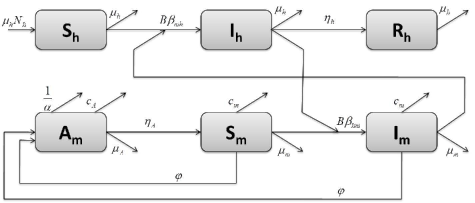
Figure 1: Epidemiological model SIR (Susceptible, Infected, Recovered) $+$ ASI (Aquatic phase, Susceptible, Infected) with $S_{h}$, $I_{h}$, $R_{h}$, $A_{m}$, $S_{m}$, and $I_{m}$ as state variables, $c_{A}$, $c_{m}$, and $\alpha$ as controls, and $N_{h}$, $B$, $\beta_{mh}$, $\beta_{hm}$, $\mu_{h}$, $\eta_{h}$, $\mu_{m}$, $\varphi$, $\mu_{A}$, $\eta_{A}$, $m$, and $k$ as given parameters.

4 Equilibrium points and the basic reproduction number

We study the solutions of System (1)–(2) in the closed set

$$\Omega=\left\{(S_{h},I_{h},R_{h},A_{m},S_{m},I_{m})\in\mathbb{R}_{+}^{6}:S_{h}+I_{h}+R_{h}\leq N_{h},\,A_{m}\leq kN_{h},\,S_{m}+I_{m}\leq mN_{h}\right\}.$$

The $\Omega$ set is positively invariant with respect to Eq. (1)–(2) (Rodrigues et al., 2012). System (1)–(2) has at most three biologically meaningful equilibrium points (cf. Theorem 2).

Definition 1.

A sextuple $E=\left(S_{h},I_{h},R_{h},A_{m},S_{m},I_{m}\right)\in\mathbb{R}^{6}$ is an equilibrium point for System (1)–(2) if it satisfies

$$\begin{cases}\mu_{h}N_{h}-\left(B\beta_{mh}\frac{I_{m}}{N_{h}}+\mu_{h}\right)S_{h}=0\\ B\beta_{mh}\frac{I_{m}}{N_{h}}S_{h}-(\eta_{h}+\mu_{h})I_{h}=0\\ \eta_{h}I_{h}-\mu_{h}R_{h}=0\\ \varphi\left(1-\frac{A_{m}}{\alpha kN_{h}}\right)(S_{m}+I_{m})-(\eta_{A}+\mu_{A}+c_{A})A_{m}=0\\ \eta_{A}A_{m}-\left(B\beta_{hm}\frac{I_{h}}{N_{h}}+\mu_{m}+c_{m}\right)S_{m}=0\\ B\beta_{hm}\frac{I_{h}}{N_{h}}S_{m}-(\mu_{m}+c_{m})I_{m}=0.\end{cases}$$ (3)

An equilibrium point $E$ is biologically meaningful if and only if $E\in\Omega$. The biologically meaningful equilibrium points are said to be disease-free or endemic depending on $I_{h}$ and $I_{m}$: if there is no disease for both populations of humans and mosquitoes ($I_{h}=I_{m}=0$), then the equilibrium point is a disease-free equilibrium (DFE); otherwise, if $I_{h}>0$ or $I_{m}>0$, then the equilibrium point is called endemic.

Theorem 2.

System (1)–(2) admits at most three biologically meaningful equilibrium points, at most two DFE points, and at most one endemic equilibrium point. Let

$$\mathcal{M}=-\left(\eta_{A}\mu_{m}+\eta_{A}c_{m}+\mu_{A}\mu_{m}+\mu_{A}c_{m}+c_{A}\mu_{m}+c_{A}c_{m}-\varphi\eta_{A}\right),$$ (4)

$$\xi=\varphi(\mu_{m}+c_{m})^{2}(\eta_{h}+\mu_{h}),\quad\chi=\alpha kB^{2}\beta_{hm}\beta_{mh}\mathcal{M},$$ (5)

$$E_{1}^{*}=\left(N_{h},0,0,0,0,0\right),\quad E_{2}^{*}=\left(N_{h},0,0,\frac{\alpha kN_{h}\mathcal{M}}{\eta_{A}\varphi},\frac{\alpha kN_{h}\mathcal{M}}{(\mu_{m}+c_{m})\varphi},0\right),$$ (6)

and $E_{3}^{*}=\left(S_{h}^{*},I_{h}^{*},R_{h}^{*},A_{m}^{*},S_{m}^{*},I_{m}^{*}\right)$ with

$$\left\{\begin{split}S_{h}^{*}&=\frac{-\varphi N_{h}(\mu_{m}\eta_{h}+\mu_{h}B\beta_{hm}+c_{m}\mu_{h}+c_{m}\eta_{h}+\mu_{m}\mu_{h})(\mu_{m}+c_{m})}{B\beta_{hm}(-\alpha kB\beta_{mh}\mathcal{M}-\varphi\mu_{h}(\mu_{m}+c_{m}))},\\ I_{h}^{*}&=\frac{\mu_{h}N_{h}\left(\xi-\chi\right)}{(\eta_{h}+\mu_{h})B\beta_{hm}(-\alpha kB\beta_{mh}\mathcal{M}-\varphi\mu_{h}(\mu_{m}+c_{m}))},\\ R_{h}^{*}&=\frac{\eta_{h}N_{h}\left(\xi-\chi\right)}{(\eta_{h}+\mu_{h})B\beta_{hm}\left(-\alpha kB\beta_{mh}\mathcal{M}-\varphi\mu_{h}(\mu_{m}+c_{m})\right)},\\ A_{m}^{*}&=\frac{N_{h}k\alpha\mathcal{M}}{\varphi\eta_{A}},\\ S_{m}^{*}&=\frac{N_{h}\mu_{h}(c_{m}+\mu_{h})(\mu_{h}+\eta_{h})}{B\beta_{mh}(\mu_{m}\eta_{h}+\mu_{h}B\beta_{hm}+c-m\mu_{h}+c_{m}\eta_{h}+\mu_{m}\mu_{h})}\\ &\qquad-\frac{N_{h}\alpha k\left(c_{m}(\mu_{h}+\eta_{h})(\mu_{A}+\eta_{A}+c_{A})+\mu_{m}(\mu_{h}(\eta_{A}+\mu_{A})+\eta_{h}(c_{A}+\eta_{A}))\right)}{\varphi(\mu_{m}\eta_{h}+\mu_{h}B\beta_{hm}+c-m\mu_{h}+c_{m}\eta_{h}+\mu_{m}\mu_{h})}\\ &\qquad-\frac{N_{h}\alpha k\left(-\eta\varphi(\mu_{h}+\eta_{h})+\mu_{m}(\eta_{h}\mu_{A}+\mu_{h}c_{A})\right)}{\varphi(\mu_{m}\eta_{h}+\mu_{h}B\beta_{hm}+c-m\mu_{h}+c_{m}\eta_{h}+\mu_{m}\mu_{h})},\\ I_{m}^{*}&=\frac{-\mu_{h}N_{h}\left(\xi-\chi\right)}{B\beta_{mh}\left(\varphi B\beta_{hm}\mu_{h}(\mu_{m}+c_{m})+\xi\right)}.\end{split}\right.$$ (7)

If $\mathcal{M}\leq 0$, then there is only one biologically meaningful equilibrium point $E_{1}^{*}$, which is a DFE point. If $\mathcal{M}>0$ with $\xi\geq\chi$, then there are two biologically meaningful equilibrium points $E_{1}^{*}$ and $E_{2}^{*}$, both DFE points. If $\mathcal{M}>0$ with $\xi<\chi$, then there are three biologically meaningful equilibrium points $E_{1}^{*}$, $E_{2}^{*}$, and $E_{3}^{*}$, where $E_{1}^{*}$ and $E_{2}^{*}$ are DFEs and $E_{3}^{*}$ is endemic.

Proof.

System (3) has four solutions obtained with the software Maple: $E_{1}^{*}$, $E_{2}^{*}$, $E_{3}^{*}$, and $E_{4}^{*}$. The equilibrium point $E_{1}^{*}$ is always a DFE because it always belong to $\Omega$ with $I_{h}=I_{m}=0$. In contrast, $E_{4}^{*}$ is never biologically realistic because it always has some negative coordinates. The other two equilibrium points, $E_{2}^{*}$ and $E_{3}^{*}$, are biologically realistic only for certain values of the parameters. The equilibrium $E_{2}^{*}$ is biologically realistic if and only if $\mathcal{M}\geq 0$, in which case it is a DFE. For the condition $\mathcal{M}\leq 0$, the third equilibrium $E_{3}^{*}$ is not biologically realistic. If $\mathcal{M}>0$, then three situations can occur with respect to $E_{3}^{*}$: if $\xi=\chi$, then $E_{3}^{*}$ degenerates into $E_{2}^{*}$, which means that $E_{3}^{*}$ is the DFE $E_{2}^{*}$; if $\xi>\chi$, then $E_{3}^{*}$ is not biologically realistic; otherwise, one has $E_{3}^{*}\in\Omega$ with $I_{h}\neq 0$ and $I_{m}\neq 0$, which means that $E_{3}^{*}$ is an endemic equilibrium point. ∎

By algebraic manipulation, $\mathcal{M}>0$ is equivalent to the condition $\displaystyle\frac{(\eta_{A}+\mu_{A}+c_{A})(\mu_{m}+c_{m})}{\varphi\eta_{A}}>1$, which is related to the number for offspring mosquitos. Thus, if $\mathcal{M}\leq 0$, then the mosquito population will collapse and the only equilibrium for the whole system is the trivial DFE $E_{1}^{*}$. If $\mathcal{M}>0$, then the mosquito population is sustainable. From a biological standpoint, the equilibrium $E_{2}^{*}$ is more plausible, because the mosquito is in its habitat, but without the disease.

Definition 3.

(Hethcote, 2008) The basic reproduction number, denoted by $\mathcal{R}_{0}$, is defined as the average number of secondary infections occurring when one infective is introduced into a completely susceptible population.

The basic reproduction number provides an invasion criterion for the initial spread of the virus in a susceptible population. For this case,

Theorem 4.

The basic reproduction number $\mathcal{R}_{0}$ associated to the differential System (1)–(2) is

$$\mathcal{R}_{0}=\left(\frac{\alpha kB^{2}\beta_{hm}\beta_{mh}\mathcal{M}}{\varphi(\eta_{h}+\mu_{h})(c_{m}+\mu_{m})^{2}}\right)^{\frac{1}{2}}=\left(\frac{\chi}{\xi}\right)^{\frac{1}{2}}.$$ (8)

Proof.

In agreement with van den Driessche and Watmough (2002), we consider the epidemiological compartments with new infections, $I_{h}$ and $I_{m}$. The two differential equations related with these two compartments are rewritten as $x^{\prime}(t)=\mathcal{F}(x(t))-\mathcal{V}(x(t))$, where $x=\left(I_{h},I_{m}\right)$, $\mathcal{F}$ is the rate of production of new infections, and $\mathcal{V}$ the transition rates between states:

$$\mathcal{F}(x)=\left(\begin{array}[]{c}B\beta_{mh}\frac{I_{m}}{N_{h}}S_{h}\\ B\beta_{hm}\frac{I_{h}}{N_{h}}S_{m}\\ \end{array}\right),\quad\mathcal{V}(x)=\left(\begin{array}[]{c}(\eta_{h}+\mu_{h})I_{h}\\ (c_{m}+\mu_{m})I_{m}\\ \end{array}\right).$$

The Jacobian derivatives are

$$J_{\mathcal{F}(x)}=\left(\begin{array}[]{cc}0&B\beta_{mh}\frac{S_{h}}{N_{h}}\\ B\beta_{hm}\frac{S_{m}}{N_{h}}&0\\ \end{array}\right),\quad J_{\mathcal{V}(x)}=\left(\begin{array}[]{cc}\eta_{h}+\mu_{h}&0\\ 0&c_{m}+\mu_{m}\\ \end{array}\right).$$

The quantity $J_{\mathcal{F}(x)}J_{\mathcal{V}(x)}^{-1}$ gives the total number of new infections over the course of an outbreak. The largest eigenvalue gives the asymptotic growth of the infected population, giving $\mathcal{R}_{0}$ as the spectral radius of the matrix $J_{\mathcal{F}(x)}J_{\mathcal{V}(x)}^{-1}$ in a DFE point. Maple was used to obtain

$$\mathcal{R}_{0}=\left(\frac{B^{2}\beta_{hm}\beta_{mh}S_{h_{\mathrm{DFE}}}S_{m_{\mathrm{DFE}}}}{(\eta_{h}+\mu_{h})(c_{m}+\mu_{m})N_{h}^{2}}\right)^{\frac{1}{2}}.$$ (9)

The basic reproduction number $\mathcal{R}_{0}$ in Eq. (8) is obtained from replacing $S_{h_{\mathrm{DFE}}}$ and $S_{m_{\mathrm{DFE}}}$ in Eq. (9) by those of the DFE $E_{2}^{*}$. ∎

The model plays on the populations of host and vector, and the expected basic reproduction number should reflect the infection transmitted from host to vector and vice-versa. Accordingly, $\mathcal{R}_{0}$ can be seen as $\mathcal{R}_{0}=(\mathcal{R}_{hm}\times\mathcal{R}_{mh})^{\frac{1}{2}}$. The infection host-vector is represented by $\mathcal{R}_{hm}=\frac{B\beta_{hm}S_{m_{\mathrm{DFE}}}}{N_{h}(\eta_{h}+\mu_{h})}$, where the term $\frac{B\beta_{hm}S_{m_{\mathrm{DFE}}}}{N_{h}}$ represents the transmission probability of the disease from humans to mosquitoes in a susceptible population of vectors, and the term $\frac{1}{\eta_{h}+\mu_{h}}$ the human viremic period. Analogously, the infection vector-host is represented by $\mathcal{R}_{mh}=\frac{B\beta_{mh}S_{h_{\mathrm{DFE}}}}{N_{h}(c_{m}+\mu_{m})}$, where $\frac{B\beta_{mh}S_{h_{\mathrm{DFE}}}}{N_{h}}$ represents the transmission of the disease from mosquito to the susceptible human population, and $\frac{1}{c_{m}+\mu_{m}}$ the lifespan of an adult mosquito.

If $\mathcal{R}_{0}<1$, on average, an infected individual produces less than one new infected individual over the course of its infectious period, and the disease declines. Conversely, if $\mathcal{R}_{0}>1$, then each individual infects more than one person, and the disease invades the population.

Theorem 5.

If $\mathcal{M}>0$ and $\mathcal{R}_{0}>1$, then System (1)–(2) admits the endemic equilibrium $E_{3}^{*}=\left(S_{h}^{*},I_{h}^{*},R_{h}^{*},A_{m}^{*},S_{m}^{*},I_{m}^{*}\right)$ given by Eq. (7).

Proof.

The only solution of Eq. (3) with $I_{h}>0$ or $I_{m}>0$, the only endemic equilibrium, is $E_{3}^{*}$. That occurs, in agreement with Theorem 2, in the case $\mathcal{M}>0$ and $\chi>\xi$. The condition $\chi>\xi$ is equivalent, by Theorem 4, to $\mathcal{R}_{0}>1$. ∎

Using the methods developed in Li and Muldowney (1996) and van den Driessche and Watmough (2002), if $\mathcal{R}_{0}\leq 1$, then the DFE is globally asymptotically stable in $\Omega$, and the vector-borne disease always dies out; if $\mathcal{R}_{0}>1$, then the unique endemic equilibrium is globally asymptotically stable in $\Omega$, so that the disease, if initially present, persists at the unique endemic equilibrium level.

5 Numerical implementation

In the epidemic of Cape Verde, infections were rising at a rate of one thousand people a day. The entire population was asked to participate in the campaign of cleaning and eradication of the mosquito, with the help of the police and the army. Data for humans are available at www.ine.cv (2011), but knowledge of mosquitoes in Africa is poor. For Aedes aegypti, Esteva and Yang (2005) and Coelho et al. (2008) have collected observations from Brazil. The simulations were carried out with $N_{h}=480,000$, $B=0.8$, $\beta_{mh}=0.375$, $\beta_{hm}=0.375$, $\mu_{h}=1/(71\times 365)$, $\eta_{h}=1/3$, $\mu_{m}=1/10$, $\mu_{m}=1/10$, $\varphi=6$, $\mu_{A}=1/4$, $\eta_{A}=0.08$, $m=3$, $k=3$. The initial conditions for the problem are: $S_{h0}=N_{h}-10$, $I_{h0}=10$, $R_{h0}=0$, $A_{m0}=kN_{h}$, $S_{m0}=mN_{h}$, $I_{m0}=0$. With these values, Eq. (4) gives $\mathcal{M}>0$. The time interval is one year and $t_{f}=365$ days. We performed all simulations and graphics with Matlab. To solve System (1)–(2), we used the ode45 routine. This function implements a Runge–Kutta method with a variable time step for efficient computation.

Figures 2a and 2b show the human and mosquito populations in the absence of any control. The human infection reached a peak between the 30th and the 50th day. The infection of the mosquitoes is delayed. The total number of infected humans obtained from System (1)–(2) is higher than observations in Cape Verde. The difference can be due to our inability to quantify individual prophylactic efforts.

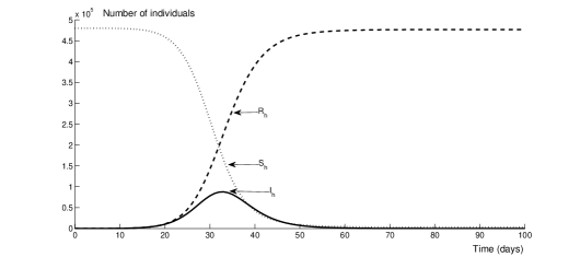
(a) Human population in the compartments Susceptible ($S_{h}$), Infected ($I_{h}$), and Recovered ($R_{h}$).

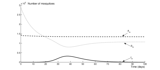
(b) Mosquito population in the compartments Aquatic phase ($A_{m}$), Susceptible ($S_{m}$), and Infected ($I_{m}$).

Figure 2: Variation of human and mosquito populations when no control is applied, i.e., for System (1)–(2) with $c_{A}=0$, $c_{m}=0$, and $\alpha=1$.

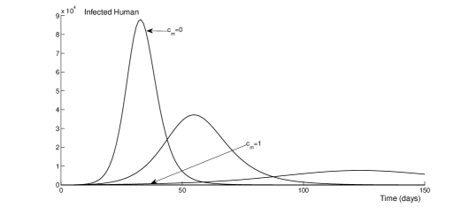
(a) Variation of infected individuals ($I_{h}$) with adulticide.

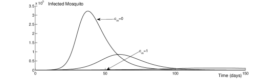
(b) Variation of infected mosquitoes ($I_{m}$) with adulticide.

Figure 3: Variation of infected human and infected mosquito populations with different levels of adulticide: $c_{m}=0$, $c_{m}=0.25$, $c_{m}=0.50$, $c_{m}=0.75$, and $c_{m}=1$. The other controls are not applied: $c_{A}=0$, and $\alpha=1$.

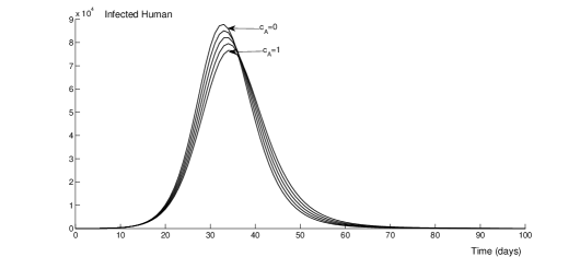
(a) Variation of infected individuals ($I_{h}$) with larvicide.

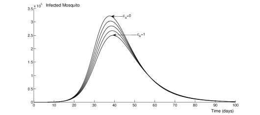
(b) Variation of infected mosquitoes ($I_{m}$) with larvicide.

Figure 4: Variation of infected human and infected mosquito populations with different levels of larvicide: $c_{A}=0$, $c_{A}=0.25$, $c_{A}=0.50$, $c_{A}=0.75$, and $c_{A}=1$. The other controls are not applied: $c_{m}=0$, and $\alpha=1$.

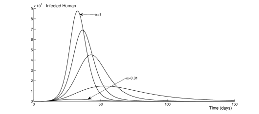
(a) Variation of infected individuals ($I_{h}$) with mechanical control.

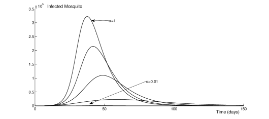
(b) Variation of infected mosquitoes ($I_{m}$) with mechanical control.

Figure 5: Variation of infected human and infected mosquito populations with different levels of mechanical control: $\alpha=0.01$, $\alpha=0.25$, $\alpha=0.5$, $\alpha=0.75$, and $\alpha=1$. The other controls are not applied: $c_{m}=0$, and $c_{A}=0$.

Figures 3a and 3b on adulticide control, Figures 4a and 4b on larvicide control, and Figures 5a and 5b on mechanical control show that a small quantity of each control is efficient to drop infection. Figures 3a and 3b show that the human population is already well protected by covering only 25% of the country with insecticide for adult mosquitoes. However, we consider that Aedes aegypti does not become resistant to insecticide and that there is no shortage of insecticide. Figures 4a, 4b, 5a, and 5b show the controls applied in the aquatic phase of the mosquito. The controls were studied separately, but each one is closely related to the other. None of these controls is sufficient to drop the total number of infected humans to zero, but the removal of breeding sites and the use of larvicide contributes to prophylaxis.

Figures 6a and 6b show simulations using the three controls simultaneously. They show that $10\%$ of each control, applied continuously, is enough to contain the infection near zero case.

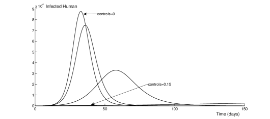
(a) Variation of infected individuals ($I_{h}$) with a combined use of the three controls.

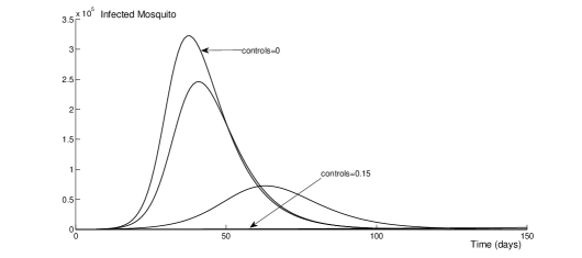
(b) Variation of infected mosquitoes ($I_{m}$) with a combined use of the three controls.

Figure 6: Variation of infected human and infected mosquito populations when using larvicide, adulticide, and mechanical control simultaneously: $c_{A}=c_{m}=1-\alpha=0$, 0.01, 0.05, 0.1, 0.15.

The eradication of Aedes aegypti may not be feasible and, from the environment point of view, not desirable. The aim is to reduce the mosquito density and increase the immunity on the humans. Population herd immunity can be reached by increasing the total number of resistant persons to the disease, which implies that these persons have been infected, or through vaccination.

No commercially available clinical cure or vaccine is currently available for dengue, but efforts are to develop one (Blaney et al., 2007; Hombach et al., 2007). Effective vaccines have been produced against other flavivirus diseases such as yellow fever, Japanese encephalitis, and tick-borne encephalitis, so there is good hope for a vaccine for dengue. We now simulate the epidemiological model with vaccination.

6 Model with vaccination

While direct individual protection is the major focus of mass vaccination program, population effects also contribute to individual protection through herd immunity, providing protection for unprotected individuals (Farrington, 2003). The more vaccinated people, the less likely a susceptible person will come into contact with the infection. With the introduction of a vaccine, the SIR model related to the human population is augmented into the SVIR model of Figure 7, where $V_{h}$ represents the total number of vaccinated people.

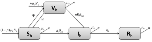
Figure 7: Epidemiological SVIR (Susceptible, Vaccinated, Infected, Recovered) model for humans with $S_{h}$, $V_{h}$ (human vaccinated population), $I_{h}$, and $R_{h}$ as state variables, $p$ (proportion of the vaccinated new born) as the control, and $N_{h}$, $B$, $\beta_{mh}$, $\mu_{h}$, $\eta_{h}$, $w$ (proportional rate at which vaccination loses effect), $\Psi$ (fraction of the vaccinated susceptible), and $\sigma$ (infection rate of vaccinated people) as given parameters.

Vaccination is continuous with a constant proportion $p$ of vaccinated new born. A fraction $\Psi$ of the susceptible is vaccinated. The vaccination reduces but does not eliminate susceptibility to infection. For this reason we consider the infection rate $\sigma$ of vaccinated people: when $\sigma=0$ the vaccine is perfect and when $\sigma=1$ the vaccine has no effect at all. The vaccination loses efficacy at a rate $w$. The differential system for the host population is:

$$\begin{cases}S_{h}^{\prime}(t)=(1-p)\mu_{h}N_{h}+wV_{h}(t)-\left(B\beta_{mh}\frac{I_{m}(t)}{N_{h}}+\Psi+\mu_{h}\right)S_{h}(t)\\ V_{h}^{\prime}(t)=p\mu_{h}N_{h}+\Psi S_{h}(t)-\left(w+\sigma B\beta_{mh}\frac{I_{m}(t)}{N_{h}}+\mu_{h}\right)V_{h}(t)\\ I_{h}^{\prime}(t)=B\beta_{mh}\frac{I_{m}(t)}{N_{h}}(S_{h}(t)+\sigma V_{h}(t))-(\eta_{h}+\mu_{h})I_{h}(t)\\ R_{h}^{\prime}(t)=\eta_{h}I_{h}(t)-\mu_{h}R_{h}(t).\end{cases}$$

Figure 8 shows simulations for decreasing vaccine efficacy. Larvicide, insecticide, and mechanical control were kept null, and the parameters $\sigma$ and $w$ were changed. For 80% of the population vaccinated, the efficacy of the vaccine reduces the disease spread.

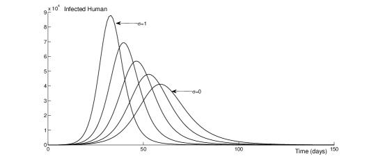
Figure 8: Total number of infected humans for decreasing vaccine efficacy ($\sigma=1-w=0$, 0.25, 0.5, 0.75, 1), $p=0.80$, and $\Psi=0.80$.

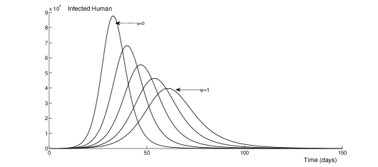
Figure 9: Total number of infected humans when using different values of population vaccinated ($\Psi=0$, 0.25, 0.5, 0.75, 1), $p=0$, $w=0.85$, and $\sigma=0.15$.

Figure 9 presents the proportion of population vaccinated. It shows that dengue fever prophylaxis articulates health and sustainable development.

7 Conclusion

Our simulations, based on our compartmental epidemiological model and formalizing clean-up campaigns to remove the vector breeding sites and the application of insecticides (larvicide and adulticide), have shown that even with a low continuous control over time, the results are encouraging. The model with an imperfect vaccine has shown that the total number of infected persons can decrease quickly.

References

- Blaney et al. (2007) Blaney, J.E., Sathe, N.S., Hanson, G.T., et al. (2007). Vaccine candidates for dengue virus type 1 (DEN1) generated by replacement of the strutural genes of rDEN4 and rDEN430 with those of DEN1. Virology Journal, 4(23): 1–11.
- Chowell et al. (2007) Chowell, G., Diaz-Duenas, P., Miller, J.C., et al. (2007). Estimation of the reproduction number of dengue fever from spatial epidemic data. Mathematical Biosciences, 208(2): 571–589.
- Christophers (2009) Christophers, S.R. (2009). Aedes aegypti, the Yellow fever Mosquito: Its Life History, Bionomics and Structure. Cambridge: Cambridge University Press.
- Coelho et al. (2008) Coelho, G., Burattini, M., Teixeira, M.G., et al. (2008). Dynamics of the 2006/2007 dengue outbreak in Brazil. Mem. Inst. Oswaldo Cruz, 103(6): 535–539.
- Derouich and Boutayeb (2006) Derouich, M. and Boutayeb, A. (2006). Dengue fever: Mathematical modelling and computer simulation. Appl. Math. Comput., 177(2): 528–544.
- Derouich et al. (2003) Derouich, M., Boutayeb, A. and Twizell, E. (2003). A model of dengue fever. Biomedical Engineering Online, 2(4): 1–10.
- Devine et al. (2009) Devine, G.J., Perea, E.Z., Killeen, G.F., et al. (2009). Using adult mosquitoes to transfer insecticides to aedes aegypti larval habitats. Proceedings of the National Academy of Sciences of the United States of America, 106(28): 11530–11534.
- Dumont and Chiroleu (2010) Dumont, Y. and Chiroleu, F. (2010). Vector control for the chikungunya disease. Mathematical Biosciences and Engineering, 7(2): 313–345.
- Dumont et al. (2008) Dumont, Y., Chiroleu, F. and Domerg, C. (2008). On a temporal model for the chikungunya disease: modeling, theory and numerics. Mathematical Biosciences, 213(1): 80–91.
- Endy et al. (2002) Endy, T.P., Chunsuttiwat, S., Nisalak, A., et al. (2002). Epidemiology of inapparent and symptomatic acute dengue virus infection: A prospective study of primary school children in Kamphaeng Phet, Thailand. Am. J. Epidemiol., 156(1): 40–51.
- Esteva and Yang (2005) Esteva, L. and Yang, H.M. (2005). Mathematical model to assess the control of aedes aegypti mosquitoes by the sterile insect technique. Mathematical Biosciences, 198(2): 132–147.
- Farrington (2003) Farrington, C. (2003). On vaccine efficacy and reproduction numbers. Mathematical Biosciences, 185(1): 89–109.
- Feng and Velasco-Hernández (1997) Feng, Z. and Velasco-Hernández, J.X. (1997). Competitie exclusion in a vector-host model for the dengue fever. Journal of Mathematical Biology, 35(5): 523–544.
- Ferreira et al. (2006) Ferreira, C.P., Pulino, P., Yang, H.M. and Takahashi, L.T. (2006). Controlling dispersal dynamics of Aedes aegypti. Mathematical Population Studies, 13(4): 215–236.
- Healstead (1992) Healstead, S.B. (1992) The XXth century dengue pandemic: need for surveillance and research. World Health Statistics Quarterly, 45(2-3): 292–298.
- Hethcote (2008) Hethcote, H.W. (2008). The basic epidemiology models: models, expressions for , parameter estimation, and applications, in Mathematical Understanding of Infectous Disease Dynamics, S. Ma, Y. Xia (eds). Lecture Notes Series Institute for Mathematical Sciences, National University of Singapore, Vol. 16, World Scientific Publishing: 1–61.
- Hombach et al. (2007) Hombach, J., Cardosa, M.J., Sabchareon, A., et al. (2007). Scientific consultation on immunological correlates of protection induced by dengue vaccines. Vaccine, 25(21): 4130–4139.
- Li and Muldowney (1996) Li, M.Y. and Muldowney, J.S. (1996). A geometric approach to global-stability problems. SIAM J. on Mathematical Analysis, 27(4): 1070–1083.
- Natal (2002) Natal, D. (2002). Bioecologia do aedes aegypti. Biológico, São Paulo, 64(2): 205–207.
- Rodrigues et al. (2009) Rodrigues, H.S., Monteiro, M.T.T. and Torres, D.F.M. (2009). Optimization of dengue epidemics: A test case with different discretization schemes. AIP Conference Proceedings, 1168(1): 1385–1388. arXiv:1001.3303
- Rodrigues et al. (2010a) Rodrigues, H.S., Monteiro, M.T.T. and Torres, D.F.M. (2010a). Dynamics of dengue epidemics when using optimal control. Mathematical and Computer Modelling, 52(9-10): 1667–1673. arXiv:1006.4392
- Rodrigues et al. (2010b) Rodrigues, H.S., Monteiro, M.T.T. and Torres, D.F.M. (2010b). Insecticide control in a dengue epidemics model. AIP Conference Proceedings, 1281(1): 979–982. arXiv:1007.5159
- Rodrigues et al. (2012) Rodrigues, H.S., Monteiro, M.T.T., Torres, D.F.M. and Zinober, A. (2012). Dengue disease, basic reproduction number and control. International Journal of Computer Mathematics, 89(3), 334–346. arXiv:1103.1923
- Scott and Morrison (2004) Scott, T.W. and Morrison, A. (2004). Aedes aegypti density and the risk of dengue-virus transmission, in Ecological aspects for application of genetically modified mosquitoes, W. Takken, T.W. Scott (eds). Springer Science, 187–206.
- Semenza and Menne (2009) Semenza, J.C. and Menne, B. (2009). Climate change and infectious diseases in Europe. The Lancet Infectious Diseases, 9(6): 365–375.
- Tewa et al. (2009) Tewa, J., Dimi, J.L. and Bowang, S. (2009). Lyapunov functions for a dengue disease transmission model. Chaos, Solitons & Fractals, 39(2): 936–941.
- Thomé et al. (2010) Thomé, R.C., Yang, H.M. and Esteva, L. (2010). Optimal control of aedes aegypti mosquitoes by the sterile techinique and insecticide. Mathematical Biosciences, 223(1): 12–23.
- van den Driessche and Watmough (2002) van den Driessche, P. and Watmough, J. (2002). Reproduction numbers and sub-threshold endemic equilibria for compartmental models of disease transmission. Mathematical Biosciences, 180(1-2), 29–48.
- www.who.int/topics/dengue/en (2011) www.who.int/topics/dengue/en. World Health Organization, accessed Sept 2011.
- www.ine.cv (2011) www.ine.cv. INE of Cape Verde, accessed Sept 2011.
- www.dengue.gov.cv (2011) www.dengue.gov.cv. Núcleo Operacional da Sociedade de Informação, Gabinete do Primeiro Ministro, accessed Sept 2011.
- www.minsaude.gov.cv (2011) www.minsaude.gov.cv. Ministério da Saúde, accessed Sept 2011.