Explicit receivers for pure-interference bosonic multiple access channels

Abstract

The pure-interference bosonic multiple access channel has two senders and one receiver, such that the senders each communicate with multiple temporal modes of a single spatial mode of light. The channel mixes the input modes from the two users pairwise on a lossless beamsplitter, and the receiver has access to one of the two output ports. In prior work, Yen and Shapiro found the capacity region of this channel if encodings consist of coherent-state preparations. Here, we demonstrate how to achieve the coherent-state Yen-Shapiro region (for a range of parameters) using a sequential decoding strategy, and we show that our strategy outperforms the rate regions achievable using conventional receivers. Our receiver performs binary-outcome quantum measurements for every codeword pair in the senders’ codebooks. A crucial component of this scheme is a non-destructive “vacuum-or-not”measurement that projects an $n$-symbol modulated codeword onto the $n$-fold vacuum state or its orthogonal complement, such that the post-measurement state is either the $n$-fold vacuum or has the vacuum removed from the support of the $n$ symbols’ joint quantum state. This receiver requires the additional ability to perform multimode optical phase-space displacements which are realizable using a beamsplitter and a laser.

One of the most important questions in quantum information theory is to determine the maximum rate at which it is possible to transmit data error-free over many independent uses of a noisy quantum channel. In the spirit of Shannon [1], this quantity is known as the classical capacity of a quantum channel because it has to do with the transmission of bits, “classical” data, over a quantum channel. Holevo, Schumacher, and Westmoreland (HSW) made partial progress on this question by providing a good lower bound on any channel’s classical capacity [2, 3]. For many channels, the HSW lower bound is equal to the capacity, but in general, it is not [4].

A channel for which the HSW lower bound is equal to the classical capacity is the pure-loss bosonic channel [5]. This capacity result follows because the HSW lower bound coincides with the Yuen-Ozawa upper bound on the channel’s classical capacity [6]. The pure-loss bosonic channel is a reasonable model of free-space or fiber-optic communication [7] and has the following Heisenberg-picture specification:

$$\hat{b}=\sqrt{\eta}\ \hat{a}+\sqrt{1-\eta}\ \hat{e},$$ (1)

where $\hat{a}$, $\hat{b}$, and $\hat{e}$ are the EM field mode operators for the sender, receiver, and environment, respectively, and $\eta\in\left[0,1\right]$ is a transmissivity parameter determining what fraction of photons make it to the receiver on average. An assumption for this channel is that the environmental input is the vacuum state. Another realistic assumption usually made when calculating this channel’s classical capacity is that the sender is constrained to have a finite mean photon-number budget of $N_{S}$ (otherwise, the channel’s classical capacity is infinite). In this case, the channel’s classical capacity is equal to $g\left(\eta N_{S}\right)$, where

$$g\left(x\right)\equiv\left(x+1\right)\log_{2}\left(x+1\right)-x\log_{2}x.$$

The authors of Ref. [5] proved that an encoding strategy for achieving the pure-loss channel’s classical capacity is to generate tensor-product coherent-state codewords randomly according to a complex, isotropic Gaussian distribution with variance $N_{S}$ (this allows the strategy to meet the mean photon budget constraint of $N_{S}$). After doing so, the codebook consists of coherent-state codewords of the form:

$$\left|\alpha^{n}\left(m\right)\right\rangle\equiv\left|\alpha_{1}\left(m\right)\right\rangle\otimes\left|\alpha_{2}\left(m\right)\right\rangle\otimes\cdots\otimes\left|\alpha_{n}\left(m\right)\right\rangle,$$ (2)

where $m\in\mathcal{M}$ indicates the classical message to be sent and $\alpha_{1}\left(m\right)$, …, $\alpha_{n}\left(m\right)\in\mathbb{C}$ (these are the independent realizations of the complex Gaussian random variable with variance $N_{S}$, where $\left|\alpha_{i}\left(m\right)\right\rangle$ is a coherent state). Recently, we showed that a sequential decoding strategy consisting of binary-outcome quantum measurements of the form

$$\left\{\left|\alpha^{n}\left(m\right)\right\rangle\left\langle\alpha^{n}\left(m\right)\right|,I^{\otimes n}-\left|\alpha^{n}\left(m\right)\right\rangle\left\langle\alpha^{n}\left(m\right)\right|\right\},$$ (3)

suffices to achieve the classical capacity of this channel [8]. This result gives an explicit, physical way to realize a capacity-achieving receiver in terms of linear-optical displacements and a coherent, non-demolition “vacuum-or-not” measurement.

A natural multi-user extension of a single-sender, single-receiver channel is one with two senders and one receiver (a multiple-access channel). Determining strategies for communication over such channels will be important for multi-user communication in free space. Yen and Shapiro considered a simple multi-user extension of the pure-loss bosonic channel in (1), and they called it the pure-interference multiple access channel (MAC) [9]. It has the following input-output Heisenberg-picture specification:

$$\hat{c}=\sqrt{\eta}\ \hat{a}+\sqrt{1-\eta}\ \hat{b},$$ (4)

where $\hat{a}$, $\hat{b}$, and $\hat{c}$ are the EM field mode operators for the first sender, the second sender, and the receiver, respectively, and $\eta\in\left[0,1\right]$ is an interference parameter determining how much the senders’ transmissions mix. In this model, the only noise that occurs is due to the mixing of the senders’ transmissions. Also, we allow the first sender a mean photon budget of $N_{S_{A}}$ and the second sender a budget of $N_{S_{B}}$.

Yen and Shapiro called the above channel the “coherent-state MAC” if the senders are restricted to using only coherent-state input codewords, and they proved the capacity region in this case has the following form:

$$R_{1} \leq g\left(\eta N_{S_{A}}\right),$$

$$R_{2} \leq g\left(\left(1-\eta\right)N_{S_{B}}\right),$$

$$R_{1}+R_{2} \leq g\left(\eta N_{S_{A}}+\left(1-\eta\right)N_{S_{B}}\right),$$ (5)

where $R_{1}$ and $R_{2}$ are the first and second senders’ communication rates, respectively. They proved this result by invoking Winter’s theorem for coding over a general quantum multiple access channel [10], and they showed that, in principle, a quantum strategy at the receiver can outperform a conventional classical strategy such as homodyne or heterodyne detection. The first sender chooses a coherent-state codebook of the form $\left\{\left|\alpha^{n}\left(l\right)\right\rangle\right\}_{l}$, and the second sender similarly chooses a codebook of the form $\left\{\left|\beta^{n}\left(m\right)\right\rangle\right\}_{m}$, with the codewords defined similarly as in (2). If the first sender chooses message $l\in\mathcal{L}$ and the second sender chooses message $m\in\mathcal{M}$, then the state produced at the output of the channel is of the form:

$$\left|\gamma^{n}\left(l,m\right)\right\rangle\equiv\left|\gamma_{1}\left(l,m\right)\right\rangle\otimes\left|\gamma_{2}\left(l,m\right)\right\rangle\otimes\cdots\otimes\left|\gamma_{n}\left(l,m\right)\right\rangle,$$ (6)

where

$$\gamma_{i}\left(l,m\right)\equiv\sqrt{\eta}\ \alpha_{i}\left(l\right)+\sqrt{1-\eta}\ \beta_{i}\left(m\right).$$ (7)

In spite of finding the above physical realization for the encoder, Yen and Shapiro left open the question of giving a physically-realizable form for a quantum receiver that achieves the above rate region.

In this paper, we prove that in some cases a sequential decoding strategy, realized explicitly with optical devices (and a multimode non-destructive vacuum or not measurement for which we do not know a structured optical realization yet), can achieve the rate region in (5) for the pure-interference bosonic multiple access channel. This sequential decoder is a natural extension of the strategy in (3) for the single-sender channel. The receiver sequentially tests pairs of codewords, by performing binary-outcome quantum measurements of the following form:

$$\left\{\left|\gamma^{n}\left(l,m\right)\right\rangle\left\langle\gamma^{n}\left(l,m\right)\right|,I^{\otimes n}-\left|\gamma^{n}\left(l,m\right)\right\rangle\left\langle\gamma^{n}\left(l,m\right)\right|\right\}.$$ (8)

The cases for which this sequential decoding strategy achieves the rates in (5) have to do with the mean-photon number constraints $N_{S_{A}}$ and $N_{S_{B}}$ and the transmissivity $\eta$, and we later outline specifically for which values of these parameters the decoder in (8) can achieve the rate region in (5).

We structure this paper as follows. In the next section, we overview some basic definitions that we use throughout the paper. In Section II, we state our main theorem regarding sequential decoding for a general pure-state multiple access channel with two classical inputs and one pure-state quantum output. This section outlines a proof of this theorem with the bulk of it appearing in Appendix C. In Section III, we apply this theorem to the pure-interference bosonic multiple access channel. Section IV discusses some cases for which a rate region achievable with sequential decoding is equivalent to the Yen-Shapiro region in (5). Finally, we conclude in Section V with a summary and some open questions.

I Notation and Definitions

We denote pure states of a quantum system $A$ with a ket $\left|\phi\right\rangle^{A}$ and the corresponding density operator as $\phi^{A}=\left|\phi\right\rangle\!\left\langle\phi\right|^{A}$. All kets that are quantum states have unit norm, and all density operators are positive semi-definite with unit trace. Let $H(A)_{\rho}\equiv-\text{Tr}\left\{\rho^{A}\log_{2}\rho^{A}\right\}$ be the von Neumann entropy of the state $\rho^{A}$. For a state $\sigma^{ABC}$, we define the quantum conditional entropy $H(A|B)_{\sigma}\equiv H(AB)_{\sigma}-H(B)_{\sigma}$ and the quantum mutual information $I(A;B)_{\sigma}\equiv H(A)_{\sigma}+H(B)_{\sigma}-H(AB)_{\sigma}.$ In order to describe the “distance” between two quantum states, we use the notion of trace distance. The trace distance between states $\sigma$ and $\rho$ is

$$\|\sigma-\rho\|_{1}=\mathrm{Tr}\left|\sigma-\rho\right|,$$

where $|X|=\sqrt{X^{\dagger}X}$. Two states that are similar have trace distance close to zero, whereas states that are perfectly distinguishable have trace distance equal to two.

The min-entropy $H_{\min}\left(B\right)_{\rho}$ of a quantum state $\rho^{B}$ is equal to the negative logarithm of its maximal eigenvalue:

$$H_{\min}\left(B\right)_{\rho}\equiv-\log_{2}\left(\inf_{\lambda\in\mathbb{R}}\left\{\lambda:\rho\leq\lambda I\right\}\right),$$

and the conditional min-entropy of a classical-quantum state $\rho^{XB}\equiv\sum_{x}p_{X}\left(x\right)\left|x\right\rangle\left\langle x\right|^{X}\otimes\rho_{x}^{B}$ with classical system $X$ and quantum system $B$ is as follows:

$$H_{\min}\left(B|X\right)_{\rho}\equiv\inf_{x\in\mathcal{X}}H_{\min}\left(B\right)_{\rho_{x}}.$$

This definition of conditional min-entropy, where the conditioning system is classical, implies the following operator inequality:

$$\forall x\ \ \ \rho_{x}^{B}\leq 2^{-H_{\min}\left(B|X\right)_{\rho}}I^{B}.$$ (9)

II General scheme for a pure-state output multiple access channel

We now prove a general result regarding rates that are achievable over a pure-state multiple access channel of the following form:

$$x,y\rightarrow\left|\phi_{x,y}\right\rangle,$$ (10)

such that Sender 1 input the letter $x$, Sender 2 inputs the letter $y$, and the receiver obtains the quantum state $\left|\phi_{x,y}\right\rangle$ at the output of the channel.

Theorem 1

Suppose that the receiver of the pure-state multiple access channel in (10) is restricted to using a sequential decoder with binary-outcome tests of the form $\left\{\left|\phi_{x^{n},y^{n}}\right\rangle\left\langle\phi_{x^{n},y^{n}}\right|,I-\left|\phi_{x^{n},y^{n}}\right\rangle\left\langle\phi_{x^{n},y^{n}}\right|\right\}$. Then the following rate region is achievable for communication over this channel:

$$R_{1} \leq H_{\min}\left(B|Y\right),$$

$$R_{2} \leq H\left(B|X\right),$$

$$R_{1}+R_{2} \leq H\left(B\right),$$ (11)

where the entropies are with respect to a classical-quantum state of the following form, for some distributions $p_{X}\left(x\right)$ and $p_{Y}\left(y\right)$:

$$\sum_{x,y}p_{X}\left(x\right)p_{Y}\left(y\right)\left|x\right\rangle\left\langle x\right|^{X}\otimes\left|y\right\rangle\left\langle y\right|^{Y}\otimes\left|\phi_{x,y}\right\rangle\left\langle\phi_{x,y}\right|^{B}.$$

Proof:

We break the proof into several parts: codebook construction, a discussion of the sequential decoder, and a detailed error analysis appearing in Appendix C.

Codebook Construction. Before communication begins, Sender 1, Sender 2, and the receiver agree upon a codebook. We allow Sender 1 to select a codebook randomly according to the distribution $p_{X}\left(x\right)$, and Sender 2 likewise to select one according to $p_{Y}\left(y\right)$. So, for every message $l\in\mathcal{L}\equiv\left\{1,\ldots,2^{nR_{1}}\right\}$, generate a codeword $x^{n}\left(l\right)\equiv x_{1}\left(l\right)\cdots x_{n}\left(l\right)$ randomly and independently according to

$$p_{X^{n}}\left(x^{n}\right)\equiv\prod\limits_{i=1}^{n}p_{X}\left(x_{i}\right).$$

Similarly, for every message $m\in\mathcal{M}\equiv\left\{1,\ldots,2^{nR_{2}}\right\}$, generate a codeword $y^{n}\left(m\right)\equiv y_{1}\left(m\right)\cdots y_{n}\left(m\right)$ randomly and independently according to

$$p_{Y^{n}}\left(y^{n}\right)\equiv\prod\limits_{i=1}^{n}p_{Y}\left(y_{i}\right).$$

Sequential Decoding. Transmitting the codewords $x^{n}\left(l\right)$ and $y^{n}\left(m\right)$ through $n$ uses of the channel $x,y\rightarrow\left|\phi_{x,y}\right\rangle$ leads to the following quantum state at the receiver’s output:

$$\left|\phi_{x^{n}\left(l\right),y^{n}\left(m\right)}\right\rangle\equiv\left|\phi_{x_{1}\left(l\right),y_{1}\left(m\right)}\right\rangle\otimes\cdots\otimes\left|\phi_{x_{n}\left(l\right),y_{n}\left(m\right)}\right\rangle.$$

Upon receiving the quantum codeword $\left|\phi_{x^{n}\left(l\right),y^{n}\left(m\right)}\right\rangle$, the receiver performs a sequence of binary-outcome quantum measurements to determine the classical codewords $x^{n}\left(l\right)$ and $y^{n}\left(m\right)$ that the senders transmitted. He first “asks,” “Is it the first codeword pair?” by performing the measurement

$$\{\phi_{x^{n}\left(1\right),y^{n}\left(1\right)},I^{\otimes n}-\phi_{x^{n}\left(1\right),y^{n}\left(1\right)}\},$$

where we abbreviate

$$\phi_{x^{n}\left(1\right),y^{n}\left(1\right)}\equiv\left|\phi_{x^{n}\left(1\right),y^{n}\left(1\right)}\right\rangle\left\langle\phi_{x^{n}\left(1\right),y^{n}\left(1\right)}\right|.$$

If he receives the outcome “yes,” then he performs no further measurements and concludes that the senders transmitted the codewords $x^{n}\left(1\right)$ and $y^{n}\left(1\right)$. If he receives the outcome “no,” then he performs the measurement

$$\{\phi_{x^{n}\left(2\right),y^{n}\left(1\right)},I^{\otimes n}-\phi_{x^{n}\left(2\right),y^{n}\left(1\right)}\}.$$

to check if the senders transmitted the second codeword pair. Similarly, he stops if he receives “yes,” and otherwise, he proceeds along similar lines. The order in which the receiver scans through the codeword pairs is

$$\left(x^{n}\left(1\right),y^{n}\left(1\right)\right) \rightarrow\cdots\rightarrow\left(x^{n}\left(\left|\mathcal{L}\right|\right),y^{n}\left(1\right)\right)\rightarrow$$

$$\left(x^{n}\left(1\right),y^{n}\left(2\right)\right) \rightarrow\cdots\rightarrow\left(x^{n}\left(\left|\mathcal{L}\right|\right),y^{n}\left(2\right)\right)\rightarrow$$

$$\cdots$$

$$\left(x^{n}\left(1\right),y^{n}\left(m\right)\right) \rightarrow\cdots\rightarrow\left(x^{n}\left(l\right),y^{n}\left(m\right)\right).$$

The rest of proof is a detailed error analysis to show that the above scheme works well. It proceeds similarly to Sen’s proof for sequential decoding of the quantum MAC [11], and as such, we put it in Appendix C. Though, the difference between our error analysis and Sen’s is that we would like to employ a sequential decoder with measurements of the form $\left\{\left|\phi_{x^{n},y^{n}}\right\rangle\left\langle\phi_{x^{n},y^{n}}\right|,I-\left|\phi_{x^{n},y^{n}}\right\rangle\left\langle\phi_{x^{n},y^{n}}\right|\right\}$, as opposed to the modified measurements that Sen employs in his proof. This will allow us to have a physically-realizable decoder for the pure-interference bosonic MAC. We clarify this point in Remark 7 of Appendix C.

∎

Corollary 2

The following rate region is also achievable, by considering a symmetric proof in which we smooth the channel to be $\Pi\Pi_{M}\phi_{L,M}\Pi_{M}\Pi$ rather than $\Pi\Pi_{L}\phi_{L,M}\Pi_{L}\Pi$ (see Appendix C). After performing a symmetric error analysis, the resulting rate region has the following form:

$$R_{1} \leq H\left(B|Y\right),\,\,\,\,\,R_{2}\leq H_{\min}\left(B|X\right),$$

$$R_{1}+R_{2} \leq H\left(B\right).$$ (12)

The convex hull of the above region and the region from Theorem 1 is always achievable because it corresponds to taking convex combinations of rate pairs from each rate region and this amounts to a time-sharing strategy. This convex hull region is equivalent to the rate region $R_{1}\leq H(B|Y),R_{2}\leq H(B|X),R_{1}+R_{2}\leq H(B)$ if the corner point

$$\left(R_{1}=\min\left\{H_{\min}\left(B|Y\right),I\left(X;B\right)\right\},R_{2}=H\left(B|X\right)\right)$$

of the region in (11) is equal to

$$\left(R_{1}=I\left(X;B\right),R_{2}=H\left(B|X\right)\right),$$

and if the corner point

$$\left(R_{1}=H\left(B|Y\right),R_{2}=\min\left\{H_{\min}\left(B|X\right),I\left(Y;B\right)\right\}\right)$$

of the region in (12) is equal to

$$\left(R_{1}=H\left(B|Y\right),R_{2}=I\left(Y;B\right)\right).$$

We consider these conditions in Section III when we reason about the rate regions achievable with sequential decoding for the pure-interference bosonic multiple access channel.

III Explicit receiver for the pure-interference bosonic multiple access channel

The strategy for achieving the capacity of the coherent-state MAC is for the two senders to induce a channel of the form in (10), by selecting $\alpha,\beta\in{\mathbb{C}}$ and preparing coherent states $\left|\alpha\right\rangle$ and $\left|\beta\right\rangle$ at the input of the channel in (4). The resulting induced channel to the receiver is of the following form:

$$\alpha,\beta\rightarrow|\sqrt{\eta}\alpha+\sqrt{1-\eta}\beta\rangle.$$

By choosing the distributions $p_{X}\left(x\right)$ and $p_{Y}\left(y\right)$ in Theorem 1 to be Gaussian as follows:

$$p_{N_{S_{A}}}\left(\alpha\right) \equiv\left({1}/{\pi}N_{S_{A}}\right)\exp\left\{{-\left|\alpha\right|^{2}}/N_{S_{A}}\right\},$$

$$p_{N_{S_{B}}}\left(\beta\right) \equiv\left({1}/{\pi}N_{S_{B}}\right)\exp\left\{{-\left|\beta\right|^{2}}/N_{S_{B}}\right\},$$

we have that the convex hull of the regions in (11) and (12) is achievable (see Corollary 2). For our case, the various entropies become as follows:

$$H\left(B|X\right) =g\left(\left(1-\eta\right)N_{S_{B}}\right),$$

$$H\left(B|Y\right) =g\left(\eta N_{S_{A}}\right),$$

$$H_{\min}\left(B|X\right) =\log_{2}\left(\left(1-\eta\right)N_{S_{B}}+1\right),$$

$$H_{\min}\left(B|Y\right) =\log_{2}\left(\eta N_{S_{A}}+1\right),$$

$$H\left(B\right) =g\left(\eta N_{S_{A}}+\left(1-\eta\right)N_{S_{B}}\right).$$

According to Corollary 2, we can show that this strategy achieves the full Yen-Shapiro region in (5) if the both of the following conditions hold

$$g\left(N^{\prime}\right)-g\left(\left(1-\eta\right)N_{S_{B}}\right) \leq\log_{2}\left(\eta N_{S_{A}}+1\right),\;{\text{and}}$$

$$g\left(N^{\prime}\right)-g\left(\eta N_{S_{A}}\right) \leq\log_{2}\left(\left(1-\eta\right)N_{S_{B}}+1\right),$$ (13)

where $N^{\prime}\equiv\eta N_{S_{A}}+\left(1-\eta\right)N_{S_{B}}$. Otherwise, the convex hull region from Corollary 2 is contained in the Yen-Shapiro region.

The quantum codebooks selected from the ensembles $\{p_{N_{S_{A}}}\left(\alpha\right),\ |\alpha\rangle\}$ and $\{p_{N_{S_{B}}}\left(\beta\right),\ |\beta\rangle\}$ have the respective forms $\left\{\left|\alpha^{n}\left(l\right)\right\rangle\right\}_{l}$ and $\left\{\left|\beta^{n}\left(m\right)\right\rangle\right\}_{m}$, with the codewords defined similarly as in (2). The sequential decoder consists of binary measurements formed from the output states in (6) for all $l\in\mathcal{L}$, $m\in\mathcal{M}$:

$$\left\{\left|\gamma^{n}\left(l,m\right)\right\rangle\left\langle\gamma^{n}\left(l,m\right)\right|,I^{\otimes n}-\left|\gamma^{n}\left(l,m\right)\right\rangle\left\langle\gamma^{n}\left(l,m\right)\right|\right\}.$$ (14)

Observing that

$$\left|\gamma^{n}\left(l,m\right)\right\rangle=D\left(\gamma_{1}\left(l,m\right)\right)\otimes\cdots\otimes D\left(\gamma_{n}\left(l,m\right)\right)\left|0\right\rangle^{\otimes n},$$

where $\gamma_{i}\left(l,m\right)$ is defined in (7), $D\left(\alpha\right)\equiv\exp\left\{\alpha\hat{a}^{{\dagger}}-\alpha^{\ast}\hat{a}\right\}$ is the well-known unitary “displacement” operator from quantum optics [12], and $\left|0\right\rangle^{\otimes n}$ is the $n$-fold tensor product vacuum state, it is clear that the decoder can implement the measurement in (14) in three steps:

1. Displace the $n$-mode codeword state by

   $$D\left(-\gamma_{1}\left(l,m\right)\right)\otimes\cdots\otimes D\left(-\gamma_{n}\left(l,m\right)\right),$$

   by employing highly asymmetric beam-splitters with a strong local oscillator [12].

2. Perform a non-destructive “vacuum-or-not” measurement of the form

   $$\left\{\left|0\right\rangle\left\langle 0\right|^{\otimes n},\ \ I^{\otimes n}-\left|0\right\rangle\left\langle 0\right|^{\otimes n}\right\}.$$

   If the vacuum outcome occurs, decode as the codeword pair $\left(l,m\right)$. Otherwise, proceed.

3. Displace by $D\left(\gamma_{1}\left(l,m\right)\right)\otimes\cdots\otimes D\left(\gamma_{n}\left(l,m\right)\right)$ with the same method as in Step 1.

The receiver just iterates this strategy for every codeword pair in the codebooks.

IV Examples

This section discusses a few examples such that the convex hull region from Corollary 2 is either equal to the full Yen-Shapiro rate region in (5) or not.

Our first example appears in Figure 1(a). By setting $\eta=1/2$, $N_{S_{A}}=1$, and $N_{S_{B}}=1$, we find that the conditions in (13) do not hold, so that the convex hull region from Corollary 2 is not equal to the full Yen-Shapiro region. Though, the convex hull region is nearly equal to the Yen-Shapiro region, and it is significantly larger than the region given by a classical strategy such as homodyne or heterodyne detection (see Ref. [9] for a discussion of the rate regions resulting from these strategies).

Our second example appears in Figure 1(b), where we set $\eta=1/2$, $N_{S_{A}}=10$, and $N_{S_{B}}=8$. We find that the conditions in (13) do hold for these values, implying that the convex hull region from Corollary 2 is equal to the full Yen-Shapiro region. Again, this region is significantly larger than the region given by a classical strategy such as homodyne or heterodyne detection.

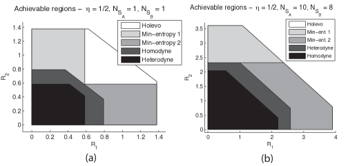
Figure 1: Rate regions achievable with various strategies at the receiving end such as Holevo joint detection (with an unrealistic square-root measurement), sequential decoding with a “vacuum-or-not” measurement according to Corollary 2, heterodyne detection, or homodyne detection. The convex hull of the regions entitled “Min-entropy 1” and “Min-entropy 2” is the region given by Corollary 2.

Figure 2 more generally captures the values of the mean input photon numbers $N_{S_{A}}$ and $N_{S_{B}}$ such that the region from Corollary 2 is equal to the Yen-Shapiro region. The figure plots these values for two fixed values of the transmissivity: $\eta=1/2$ and $\eta=4/5$. A simple observation is that the regions are equivalent for higher mean input photon numbers. This result follows because the min-entropy boundaries are equivalent to the some of the boundaries in the heterodyne detection region (c.f., Ref. [9]), and we know that heterodyne detection becomes optimal in the high photon-number limit.

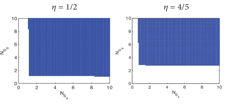
Figure 2: The shaded region indicates the values of the mean input photon numbers $N_{S_{A}}$ and $N_{S_{B}}$ such that the region from Corollary 2 is equal to the Yen-Shapiro region.

V Conclusion

We have provided a near-explicit physically-realizable optical receiver such that two senders and a receiver can achieve, in some cases, the Yen-Shapiro rate region in (5) for the pure-interference bosonic multiple access channel. The scheme has the receiver perform binary-outcome quantum tests for every codeword pair in the two codebooks of the senders. It is possible to implement this strategy with unitary displacements (realizable using a bank of highly-transmissive beamsplitters and strong coherent-state local oscillators), and a “vacuum-or-not” measurement (for which an all-optical structured realization still eludes us). However, there is a suggestion for realizing this measurement using an atom-optical coupled system with adiabatic STIRAP pulses [13].

There are many open questions to consider. First, it seems natural to conjecture that the sequential decoding algorithm in Section III should be able to achieve the full Yen-Shapiro rate region. It is a bit odd that its performance should depend on the particular mathematical error analysis employed, either that in Theorem 1 or Corollary 2, given that the physical procedure for decoding is the same in both cases. It is very likely our error analysis that is lacking, and we think that an eventual proof of the “quantum simultaneous decoding conjecture” from Ref. [14] might resolve this issue.

Yen and Shapiro found that employing squeezed states for an encoding could achieve rates beyond the coherent-state region in (5) for the same values of $\eta$, $N_{S_{A}}$, and $N_{S_{B}}$ [9]. It would be interesting to develop a physically-realizable sequential decoding strategy for this case. Though, it is not clear to us how to do so because the state at the output of the channel in (4) in this case will be a mixed state, and as of now, we do not know how to realize such a decoder with optical devices.

One can also achieve the rate region of the multiple access channel with a successive decoder [10], in which the receiver first decodes one sender’s message before decoding the other sender’s message. It is of course possible to do this in principle, but it is not clear to us how to implement such a decoder with optical devices. If we knew how to realize a sequential decoder for the channel in (1) where the environment injects thermal noise, then this should lead to an implementation of a successive decoder for the pure-interference bosonic multiple access channel.

Finally, it is open to find a physically-realizable sequential decoding scheme for an entanglement-assisted bosonic multiple access channel, for which an achievable rate region was given in Ref. [15]. It is also open to determine a physically-realizable decoder for the bosonic multiple access channel with thermal noise [9], the bosonic broadcast channel [16, 17], and the bosonic quantum interference channel [18]. The authors thank Ivan Savov for a helpful discussion.

Appendix A Typical Sequences and Typical Subspaces

Consider a density operator $\rho$ with the following spectral decomposition:

$$\rho=\sum_{x}p_{X}\left(x\right)\left|x\right\rangle\left\langle x\right|.$$

The weakly typical subspace is defined as the span of all vectors such that the sample entropy $\overline{H}\left(x^{n}\right)$ of their classical label is close to the true entropy $H\left(X\right)$ of the distribution $p_{X}\left(x\right)$ [19, 20]:

$$T_{\delta}^{X^{n}}\equiv\text{span}\left\{\left|x^{n}\right\rangle:\left|\overline{H}\left(x^{n}\right)-H\left(X\right)\right|\leq\delta\right\},$$

where

$$\overline{H}\left(x^{n}\right) \equiv-\frac{1}{n}\log\left(p_{X^{n}}\left(x^{n}\right)\right),$$

$$H\left(X\right) \equiv-\sum_{x}p_{X}\left(x\right)\log p_{X}\left(x\right).$$

The projector $\Pi_{\rho,\delta}^{n}$ onto the typical subspace of $\rho$ is defined as

$$\Pi_{\rho,\delta}^{n}\equiv\sum_{x^{n}\in T_{\delta}^{X^{n}}}\left|x^{n}\right\rangle\left\langle x^{n}\right|,$$

where we have “overloaded” the symbol $T_{\delta}^{X^{n}}$ to refer also to the set of $\delta$-typical sequences:

$$T_{\delta}^{X^{n}}\equiv\left\{x^{n}:\left|\overline{H}\left(x^{n}\right)-H\left(X\right)\right|\leq\delta\right\}.$$

The three important properties of the typical projector are as follows:

$$\text{Tr}\left\{\Pi_{\rho,\delta}^{n}\rho^{\otimes n}\right\} \geq 1-\epsilon,$$ (15)

$$\text{Tr}\left\{\Pi_{\rho,\delta}^{n}\right\} \leq 2^{n\left[H\left(X\right)+\delta\right]},$$

$$2^{-n\left[H\left(X\right)+\delta\right]}\ \Pi_{\rho,\delta}^{n} \leq\Pi_{\rho,\delta}^{n}\ \rho^{\otimes n}\ \Pi_{\rho,\delta}^{n}\leq 2^{-n\left[H\left(X\right)-\delta\right]}\ \Pi_{\rho,\delta}^{n},$$ (16)

where the first property holds for arbitrary $\epsilon,\delta>0$ and sufficiently large $n$. Consider an ensemble $\left\{p_{X}\left(x\right),\rho_{x}\right\}_{x\in\mathcal{X}}$ of states. Suppose that each state $\rho_{x}$ has the following spectral decomposition:

$$\rho_{x}=\sum_{y}p_{Y|X}\left(y|x\right)\left|y_{x}\right\rangle\left\langle y_{x}\right|.$$

Consider a density operator $\rho_{x^{n}}$ which is conditional on a classical sequence $x^{n}\equiv x_{1}\cdots x_{n}$:

$$\rho_{x^{n}}\equiv\rho_{x_{1}}\otimes\cdots\otimes\rho_{x_{n}}.$$

We define the weak conditionally typical subspace as the span of vectors (conditional on the sequence $x^{n}$) such that the sample conditional entropy $\overline{H}\left(y^{n}|x^{n}\right)$ of their classical labels is close to the true conditional entropy $H\left(Y|X\right)$ of the distribution $p_{Y|X}\left(y|x\right)p_{X}\left(x\right)$ [19, 20]:

$$T_{\delta}^{Y^{n}|x^{n}}\equiv\text{span}\left\{\left|y_{x^{n}}^{n}\right\rangle:\left|\overline{H}\left(y^{n}|x^{n}\right)-H\left(Y|X\right)\right|\leq\delta\right\},$$

where

$$\overline{H}\left(y^{n}|x^{n}\right) \equiv-\frac{1}{n}\log\left(p_{Y^{n}|X^{n}}\left(y^{n}|x^{n}\right)\right),$$

$$H\left(Y|X\right) \equiv-\sum_{x}p_{X}\left(x\right)\sum_{y}p_{Y|X}\left(y|x\right)\log p_{Y|X}\left(y|x\right).$$

The projector $\Pi_{\rho_{x^{n}},\delta}$ onto the weak conditionally typical subspace of $\rho_{x^{n}}$ is as follows:

$$\Pi_{\rho_{x^{n}},\delta}\equiv\sum_{y^{n}\in T_{\delta}^{Y^{n}|x^{n}}}\left|y_{x^{n}}^{n}\right\rangle\left\langle y_{x^{n}}^{n}\right|,$$

where we have again overloaded the symbol $T_{\delta}^{Y^{n}|x^{n}}$ to refer to the set of weak conditionally typical sequences:

$$T_{\delta}^{Y^{n}|x^{n}}\equiv\left\{y^{n}:\left|\overline{H}\left(y^{n}|x^{n}\right)-H\left(Y|X\right)\right|\leq\delta\right\}.$$

The three important properties of the weak conditionally typical projector are as follows:

$$\mathbb{E}_{X^{n}}\left\{\text{Tr}\left\{\Pi_{\rho_{X^{n}},\delta}\rho_{X^{n}}\right\}\right\} \geq 1-\epsilon,$$ (17)

$$\text{Tr}\left\{\Pi_{\rho_{x^{n}},\delta}\right\} \leq 2^{n\left[H\left(Y|X\right)+\delta\right]},$$ (18)

$$2^{-n\left[H\left(Y|X\right)+\delta\right]}\ \Pi_{\rho_{x^{n}},\delta} \leq\Pi_{\rho_{x^{n}},\delta}\ \rho_{x^{n}}\ \Pi_{\rho_{x^{n}},\delta}$$ (19)

$$\leq 2^{-n\left[H\left(Y|X\right)-\delta\right]}\ \Pi_{\rho_{x^{n}},\delta},$$

where the first property holds for arbitrary $\epsilon,\delta>0$ and sufficiently large $n$, and the expectation is with respect to the distribution $p_{X^{n}}\left(x^{n}\right)$.

Appendix B Useful lemmas

Here we collect some useful lemmas.

Lemma 3 (Gentle Operator Lemma [21, 22])

Let $\Lambda$ be a positive operator where $0\leq\Lambda\leq I$ (usually $\Lambda$ is a POVM element), $\rho$ a state, and $\epsilon$ a positive number such that the probability of detecting the outcome $\Lambda$ is high:

$$\text{Tr}\left\{\Lambda\rho\right\}\geq 1-\epsilon.$$

Then the measurement causes little disturbance to the state $\rho$:

$$\left\|\rho-\sqrt{\Lambda}\rho\sqrt{\Lambda}\right\|_{1}\leq 2\sqrt{\epsilon}.$$

The following lemma appears in Refs. [21, 22, 20].

Lemma 4 (Gentle Operator Lemma for Ensembles)

Given an ensemble $\left\{p_{X}\left(x\right),\rho_{x}\right\}$ with expected density operator $\rho\equiv\sum_{x}p_{X}\left(x\right)\rho_{x}$, suppose that an operator $\Lambda$ such that $I\geq\Lambda\geq 0$ succeeds with high probability on the state $\rho$:

$$\text{Tr}\left\{\Lambda\rho\right\}\geq 1-\epsilon.$$

Then the subnormalized state $\sqrt{\Lambda}\rho_{x}\sqrt{\Lambda}$ is close in expected trace distance to the original state $\rho_{x}$:

$$\mathbb{E}_{X}\left\{\left\|\sqrt{\Lambda}\rho_{X}\sqrt{\Lambda}-\rho_{X}\right\|_{1}\right\}\leq 2\sqrt{\epsilon}.$$

Lemma 5

Let $\rho$ and $\sigma$ be positive operators and $\Lambda$ a positive operator such that $0\leq\Lambda\leq I$. Then the following inequality holds

$$\text{Tr}\left\{\Lambda\rho\right\}\leq\text{Tr}\left\{\Lambda\sigma\right\}+\left\|\rho-\sigma\right\|_{1}.$$

Lemma 6 (Non-commutative union bound [11])

Let $\sigma$ be a subnormalized state such that $\sigma\geq 0$ and Tr$\left\{\sigma\right\}\leq 1$. Let $\Pi_{1}$, …, $\Pi_{N}$ be projectors. Then the following “non-commutative union bound” holds

$$\text{Tr}\left\{\sigma\right\}-\text{Tr}\left\{\Pi_{N}\cdots\Pi_{1}\sigma\Pi_{1}\cdots\Pi_{N}\right\}\leq 2\sqrt{\sum_{i=1}^{N}\text{Tr}\left\{\left(I-\Pi_{i}\right)\sigma\right\}}.$$

Appendix C Proof of main theorem

Error Analysis. Suppose that Sender 1 transmits the $l^{\text{th}}$ codeword and that Sender 2 transmits the $m^{\text{th}}$ codeword. Then the probability for the receiver to decode correctly with the above sequential decoding strategy is as follows:

$$\text{Tr}\left\{\phi_{l,m}\hat{\Pi}_{l-1,m}\cdots\hat{\Pi}_{1,1}\phi_{l,m}\hat{\Pi}_{1,1}\cdots\hat{\Pi}_{l-1,m}\phi_{l,m}\right\},$$

where we make the abbreviations

$$\phi_{l,m} \equiv\left|\phi_{x^{n}\left(l\right),y^{n}\left(m\right)}\right\rangle\left\langle\phi_{x^{n}\left(l\right),y^{n}\left(m\right)}\right|,$$

$$\hat{\Pi}_{l,m} \equiv I-\phi_{l,m}.$$

The above probability corresponds to the case that the receiver receives “no” answers when he performs the measurements for the 1st codeword pair $\left(x^{n}\left(1\right),y^{n}\left(1\right)\right)$ all the way until the codeword pair $\left(x^{n}\left(l-1\right),y^{n}\left(m\right)\right)$ and he then receives a “yes” answer for the codeword pair $\left(x^{n}\left(l\right),y^{n}\left(m\right)\right)$. So, the probability that the receiver decodes the pair $\left(l,m\right)$ incorrectly is

$$1-\text{Tr}\left\{\phi_{l,m}\hat{\Pi}_{l-1,m}\cdots\hat{\Pi}_{1,1}\phi_{l,m}\hat{\Pi}_{1,1}\cdots\hat{\Pi}_{l-1,m}\phi_{l,m}\right\}.$$

In order to simplify the error analysis, we analyze the expectation of the above error probability, by assuming that both senders choose their messages uniformly at random and furthermore that the codewords are selected at random independently and identically according to the distributions $p_{X}\left(x\right)$ and $p_{Y}\left(y\right)$ (as described above):

$$1-\mathbb{E}\text{Tr}\left\{\phi_{L,M}\hat{\Pi}_{L-1,M}\cdots\hat{\Pi}_{1,1}\phi_{L,M}\hat{\Pi}_{1,1}\cdots\hat{\Pi}_{L-1,M}\phi_{L,M}\right\}.$$ (20)

In the above and for the rest of the proof, it is implicit that the expectation $\mathbb{E}$ is with respect to the random variables $X^{n}$, $Y^{n}$, $L$, and $M$, unless otherwise stated.

We first observe that it is possible to consider a slightly altered channel for which we are coding. Instead of decoding the original channel $\left|\phi_{x^{n}\left(l\right),y^{n}\left(m\right)}\right\rangle$, we can decode a projected channel of the form $\Pi\Pi_{l}\left|\phi_{x^{n}\left(l\right),y^{n}\left(m\right)}\right\rangle$, where we define the projectors $\Pi$ and $\Pi_{l}$ below. That we can do so follows from the inequalities below:

$$1 =\mathbb{E}\text{Tr}\left\{\phi_{L,M}\right\}$$

$$=\mathbb{E}\text{Tr}\left\{\Pi_{L}\phi_{L,M}\right\}+\mathbb{E}\text{Tr}\{\hat{\Pi}_{L}\phi_{L,M}\}$$

$$=\mathbb{E}\text{Tr}\left\{\Pi_{L}\phi_{L,M}\Pi_{L}\right\}+\mathbb{E}_{X^{n},L,M}\text{Tr}\{\hat{\Pi}_{L}\mathbb{E}_{Y^{n}}\left\{\phi_{L,M}\right\}\}$$

$$=\mathbb{E}\text{Tr}\left\{\Pi_{L}\phi_{L,M}\Pi_{L}\right\}+\mathbb{E}_{X^{n},L,M}\text{Tr}\{\hat{\Pi}_{L}\rho_{L}\}$$

$$\leq\mathbb{E}\text{Tr}\left\{\Pi\Pi_{L}\phi_{L,M}\Pi_{L}\right\}+\mathbb{E}\text{Tr}\left\{\hat{\Pi}\Pi_{L}\phi_{L,M}\Pi_{L}\right\}+\mathbb{\epsilon}$$

$$\leq\mathbb{E}\text{Tr}\left\{\Pi\Pi_{L}\phi_{L,M}\Pi_{L}\Pi\right\}+\mathbb{E}\text{Tr}\left\{\hat{\Pi}\phi_{L,M}\right\}$$

$$\ \ \ \ +\mathbb{E}\left\|\phi_{L,M}-\Pi_{L}\phi_{L,M}\Pi_{L}\right\|_{1}+\mathbb{\epsilon}$$

$$\leq\mathbb{E}\text{Tr}\left\{\Pi\Pi_{L}\phi_{L,M}\Pi_{L}\Pi\right\}+\text{Tr}\left\{\hat{\Pi}\mathbb{E}\left\{\phi_{L,M}\right\}\right\}+2\sqrt{\mathbb{\epsilon}}+\mathbb{\epsilon}$$

$$=\mathbb{E}\text{Tr}\left\{\Pi\Pi_{L}\phi_{L,M}\Pi_{L}\Pi\right\}+\text{Tr}\left\{\hat{\Pi}\rho^{\otimes n}\right\}+2\sqrt{\mathbb{\epsilon}}+\mathbb{\epsilon}$$

$$\leq\mathbb{E}\text{Tr}\left\{\Pi\Pi_{L}\phi_{L,M}\Pi_{L}\Pi\right\}+2\sqrt{\mathbb{\epsilon}}+2\mathbb{\epsilon}$$

In the second equality, the projector $\Pi_{L}$ is a weak conditionally typical projector corresponding to the following state:

$$\mathbb{E}_{Y^{n}}\left\{\left|\phi_{X^{n}\left(L\right),Y^{n}\left(M\right)}\right\rangle\left\langle\phi_{X^{n}\left(L\right),Y^{n}\left(M\right)}\right|\right\}.$$

(See Appendix A for an explanation.) The first inequality follows from applying the property (17) of weak conditionally typical subspaces. Also, we bring in the weak typical projector (defined as $\Pi$) for the following state:

$$\mathbb{E}_{X^{n}Y^{n}}\left\{\left|\phi_{X^{n}\left(L\right),Y^{n}\left(M\right)}\right\rangle\left\langle\phi_{X^{n}\left(L\right),Y^{n}\left(M\right)}\right|\right\}.$$

The second inequality follows by applying the trace inequality from Lemma 5. The third inequality follows from the Gentle Operator Lemma for Ensembles and the property (17) of weak conditionally typical subspaces. The final inequality follows from the property (15) of weakly typical subspaces.

Consider also the following lower bound:

$$\mathbb{E}\text{Tr}\left\{\phi_{L,M}\hat{\Pi}_{L-1,M}\cdots\hat{\Pi}_{1,1}\phi_{L,M}\hat{\Pi}_{1,1}\cdots\hat{\Pi}_{L-1,M}\phi_{L,M}\right\}$$

$$=\mathbb{E}\text{Tr}\left\{\hat{\Pi}_{1,1}\cdots\hat{\Pi}_{L-1,M}\phi_{L,M}\hat{\Pi}_{L-1,M}\cdots\hat{\Pi}_{1,1}\phi_{L,M}\right\}$$

$$\geq\mathbb{E}\text{Tr}\{\hat{\Pi}_{1,1}\cdots\hat{\Pi}_{L-1,M}\phi_{L,M}\hat{\Pi}_{L-1,M}\cdots\hat{\Pi}_{1,1}\Pi\Pi_{L}\phi_{L,M}\Pi_{L}\Pi\}$$

$$\ \ \ \ -\mathbb{E}\left\|\Pi_{L}\phi_{L,M}\Pi_{L}-\phi_{L,M}\right\|_{1}$$

$$\ \ \ \ -\mathbb{E}\left\|\Pi\phi_{L,M}\Pi-\phi_{L,M}\right\|_{1}$$

$$\geq\mathbb{E}\text{Tr}\left\{\hat{\Pi}_{1,1}\cdots\hat{\Pi}_{L-1,M}\phi_{L,M}\hat{\Pi}_{L-1,M}\cdots\hat{\Pi}_{1,1}\Pi\Pi_{L}\phi_{L,M}\Pi_{L}\Pi\right\}$$

$$\ \ \ \ -4\sqrt{\epsilon}.$$

The first equality is from cyclicity of trace. The first inequality follows from two applications of the trace inequality (Lemma 5). The final inequality follows from the properties of typical subspaces. Putting all of this together gives us the following upper bound on the error probability in (20):

$$\mathbb{E}\text{Tr}\left\{\Pi\Pi_{L}\phi_{L,M}\Pi_{L}\Pi\right\}\\ -\mathbb{E}\text{Tr}\{\phi_{L,M}\hat{\Pi}_{L-1,M}\cdots\hat{\Pi}_{1,1}\Pi\Pi_{L}\phi_{L,M}\Pi_{L}\Pi\hat{\Pi}_{1,1}\cdots\hat{\Pi}_{L-1,M}\}\\ +2\mathbb{\epsilon}+6\sqrt{\epsilon}.$$

We now apply Sen’s non-commutative union bound (Lemma  of Ref. [11] or Lemma 6 of Appendix B) and concavity of the square-root function to obtain the following upper bound on the error probability:

$$2\left(\begin{array}[c]{l}\mathbb{E}\text{Tr}\left\{\left(I-\phi_{L,M}\right)\Pi\Pi_{L}\phi_{L,M}\Pi_{L}\Pi\right\}\\ \ \ \ \ \ +\mathbb{E}\sum_{\left(i,j\right)<\left(L,M\right)}\text{Tr}\left\{\phi_{i,j}\Pi\Pi_{L}\phi_{L,M}\Pi_{L}\Pi\right\}\end{array}\right)^{\frac{1}{2}}\\ \leq 2\left(\begin{array}[c]{l}\mathbb{E}\text{Tr}\left\{\left(I-\phi_{L,M}\right)\Pi\Pi_{L}\phi_{L,M}\Pi_{L}\Pi\right\}\\ \ \ \ \ \ +\mathbb{E}\sum_{\left(i,j\right)\neq\left(L,M\right)}\text{Tr}\left\{\phi_{i,j}\Pi\Pi_{L}\phi_{L,M}\Pi_{L}\Pi\right\}\end{array}\right)^{\frac{1}{2}}.$$

We handle each of these error terms individually. We upper bound the first term:

$$\mathbb{E}\text{Tr}\left\{\left(I-\phi_{L,M}\right)\Pi\Pi_{L}\phi_{L,M}\Pi_{L}\Pi\right\}$$

$$\leq\mathbb{E}\text{Tr}\left\{\left(I-\phi_{L,M}\right)\phi_{L,M}\right\}$$

$$\ \ \ \ +\mathbb{E}\left\|\Pi_{L}\phi_{L,M}\Pi_{L}-\phi_{L,M}\right\|_{1}+\mathbb{E}\left\|\Pi\phi_{L,M}\Pi-\phi_{L,M}\right\|_{1}$$

$$\leq 4\sqrt{\epsilon}.$$

The inequalities follow from the trace inequality, the properties of typical subspaces, and the Gentle Operator Lemma for Ensembles. We can split the second term into three different ones as follows:

$$\mathbb{E}\sum_{\left(i,j\right)\neq\left(L,M\right)}\left(\cdot\right)=\mathbb{E}\sum_{i\neq L}\left(\cdot\right)+\mathbb{E}\sum_{j\neq M}\left(\cdot\right)+\mathbb{E}\sum_{i\neq L,j\neq M}\left(\cdot\right).$$

We handle each of these three terms separately. Consider the first term:

$$\mathbb{E}\sum_{i\neq L}\text{Tr}\left\{\phi_{i,M}\Pi\Pi_{L}\phi_{L,M}\Pi_{L}\Pi\right\}$$

$$=\mathbb{E}_{Y^{n},L,M}\sum_{i\neq L}\mathbb{E}_{X^{n}}\text{Tr}\left\{\phi_{i,M}\Pi\Pi_{L}\phi_{L,M}\Pi_{L}\Pi\right\}$$

$$=\mathbb{E}_{Y^{n},L,M}\sum_{i\neq L}\text{Tr}\left\{\mathbb{E}_{X^{n}}\left\{\phi_{i,M}\right\}\Pi\Pi_{L}\mathbb{E}_{X^{n}}\left\{\phi_{L,M}\right\}\Pi_{L}\Pi\right\}$$

$$=\mathbb{E}_{Y^{n},L,M}\sum_{i\neq L}\text{Tr}\left\{\rho_{M}\Pi\Pi_{L}\rho_{M}\Pi_{L}\Pi\right\}$$

$$\leq 2^{-nH_{\min}\left(B|Y\right)}\mathbb{E}_{Y^{n},L,M}\sum_{i\neq L}\text{Tr}\left\{\rho_{M}\Pi\Pi_{L}\Pi\right\}$$

$$\leq 2^{-nH_{\min}\left(B|Y\right)}\left|\mathcal{L}\right|$$ (21)

The first equality follows by bringing the expectation $\mathbb{E}_{X^{n}}$ inside the sum. The second equality follows because the random variables $X^{n}\left(i\right)$ and $X^{n}\left(L\right)$ are independent and so the expectation $\mathbb{E}_{X^{n}}$ distributes. The third equality follows by evaluating the expectations by defining $\rho_{M}$ to be as follows:

$$\rho_{M}\equiv\mathbb{E}_{X^{n}}\left\{\left|\phi_{X^{n}\left(L\right),Y^{n}\left(M\right)}\right\rangle\left\langle\phi_{X^{n}\left(L\right),Y^{n}\left(M\right)}\right|\right\}.$$

The first inequality follows by bounding the largest eigenvalue of $\rho_{M}$ by the min-entropy $2^{-nH_{\min}\left(B|Y\right)}$. The second inequality follows because Tr$\left\{\rho_{M}\Pi\Pi_{L}\Pi\right\}\leq 1$.

We handle the second term:

$$\mathbb{E}\sum_{j\neq M}\text{Tr}\left\{\phi_{L,j}\Pi\Pi_{L}\phi_{L,M}\Pi_{L}\Pi\right\}$$

$$=\mathbb{E}_{X^{n},L,M}\sum_{j\neq M}\mathbb{E}_{Y^{n}}\text{Tr}\left\{\phi_{L,j}\Pi\Pi_{L}\phi_{L,M}\Pi_{L}\Pi\right\}$$

$$=\mathbb{E}_{X^{n},L,M}\sum_{j\neq M}\text{Tr}\left\{\mathbb{E}_{Y^{n}}\left\{\phi_{L,j}\right\}\Pi\Pi_{L}\mathbb{E}_{Y^{n}}\left\{\phi_{L,M}\right\}\Pi_{L}\Pi\right\}$$

$$=\mathbb{E}_{X^{n},L,M}\sum_{j\neq M}\text{Tr}\left\{\rho_{L}\Pi\Pi_{L}\rho_{L}\Pi_{L}\Pi\right\}$$

$$\leq 2^{-n\left[H\left(B|X\right)-\delta\right]}\mathbb{E}_{X^{n},L,M}\sum_{j\neq M}\text{Tr}\left\{\rho_{L}\Pi\Pi_{L}\Pi\right\}$$

$$\leq 2^{-n\left[H\left(B|X\right)-\delta\right]}\left|\mathcal{M}\right|.$$

The first four equalities follow for reasons similar to the above. The first inequality is from the typical projector bound in (19). The last inequality follows because Tr$\left\{\rho_{L}\Pi\Pi_{L}\Pi\right\}\leq 1$. Finally, we handle the third term:

$$\mathbb{E}\sum_{i\neq L,j\neq M}\text{Tr}\left\{\phi_{i,j}\Pi\Pi_{L}\phi_{L,M}\Pi_{L}\Pi\right\}$$

$$=\mathbb{E}_{X^{n},L,M}\sum_{i\neq L,j\neq M}\text{Tr}\left\{\rho_{i}\Pi\Pi_{L}\rho_{L}\Pi_{L}\Pi\right\}$$

$$\leq\mathbb{E}_{X^{n},L,M}\sum_{i\neq L,j\neq M}\text{Tr}\left\{\rho_{i}\Pi\rho_{L}\Pi\right\}$$

$$=\mathbb{E}_{L,M}\sum_{i\neq L,j\neq M}\text{Tr}\left\{\mathbb{E}_{X^{n}}\left\{\rho_{i}\right\}\Pi\mathbb{E}_{X^{n}}\left\{\rho_{L}\right\}\Pi\right\}$$

$$=\mathbb{E}_{L,M}\sum_{i\neq L,j\neq M}\text{Tr}\left\{\rho^{\otimes n}\Pi\rho^{\otimes n}\Pi\right\}$$

$$\leq 2^{-n\left[H\left(B\right)-\delta\right]}\mathbb{E}_{L,M}\sum_{i\neq L,j\neq M}\text{Tr}\left\{\rho^{\otimes n}\Pi\right\}$$

$$\leq 2^{-n\left[H\left(B\right)-\delta\right]}\left|\mathcal{L}\right|\left|\mathcal{M}\right|.$$

The first inequality follows for reasons similar to the above ones. The first inequality follows because $\Pi_{L}\rho_{L}\Pi_{L}\leq\rho_{L}$. The second equality follows from distributing the expectation over $X^{n}$. The second inequality follows from the typical projector bound in (16). The final inequality follows because Tr$\left\{\rho^{\otimes n}\Pi\right\}\leq 1$.

Thus, the overall upper bound on the error probability with this sequential decoding strategy is

$$6\epsilon+2\sqrt{\epsilon}+2\big{(}4\sqrt{\epsilon}+2^{-nH_{\min}\left(B|Y\right)}\left|\mathcal{L}\right|\\ +2^{-n\left[H\left(B|X\right)-\delta\right]}\left|\mathcal{M}\right|+2^{-n\left[H\left(B\right)-\delta\right]}\left|\mathcal{L}\right|\left|\mathcal{M}\right|\big{)}^{1/2},$$ (22)

which we can make arbitrarily small by choosing the rates to be in the region given in the statement of Theorem 1 and taking $n$ sufficiently large. We proved a bound on the expectation of the average probability, which implies there exists a particular code that has arbitrarily small average error probability under the same choice of $\left|\mathcal{L}\right|$, $\left|\mathcal{M}\right|$, and $n$.

Remark 7

One can achieve the following rate region with von Neumann entropies by employing an idea similar to that of Sen in Ref. [11]:

$$R_{1}\leq H\left(B|Y\right),\ \ \ R_{2}\leq H\left(B|X\right),\ \ \ R_{1}+R_{2}\leq H\left(B\right).$$ (23)

Indeed, the idea is to perform sequential decoding measurements of the following form:

$$\{\phi_{x^{n}\left(l\right),y^{n}\left(m\right)}^{\prime},I^{\otimes n}-\phi_{x^{n}\left(l\right),y^{n}\left(m\right)}^{\prime}\},$$ (24)

where

$$|\phi_{x^{n}\left(l\right),y^{n}\left(m\right)}^{\prime}\rangle\equiv\frac{1}{\left\|\Pi_{m}\left|\phi_{x^{n}\left(l\right),y^{n}\left(m\right)}\right\rangle\right\|_{2}}\Pi_{m}\left|\phi_{x^{n}\left(l\right),y^{n}\left(m\right)}\right\rangle,$$

and $\Pi_{m}$ is a typical projector for the state $\mathbb{E}_{X^{n}}\left\{\phi_{X^{n}\left(l\right),y^{n}\left(m\right)}\right\}$. The following bound holds for the norm $\left\|\Pi_{m}\left|\phi_{x^{n}\left(l\right),y^{n}\left(m\right)}\right\rangle\right\|_{2}^{2}\geq 1-\sqrt{\epsilon}$, due to the properties of quantum typicality (one requires strong typicality here, but this is a minor point). After applying Sen’s bound, one can invoke the following operator inequality:

$$\phi_{x^{n}\left(l\right),y^{n}\left(m\right)}^{\prime}$$

$$=\left(\left\|\Pi_{m}\left|\phi_{x^{n}\left(l\right),y^{n}\left(m\right)}\right\rangle\right\|_{2}^{2}\right)^{-1}\Pi_{m}\ \phi_{x^{n}\left(l\right),y^{n}\left(m\right)}\ \Pi_{m}$$

$$\leq\left(1-\sqrt{\epsilon}\right)^{-1}\Pi_{m}\ \phi_{x^{n}\left(l\right),y^{n}\left(m\right)}\ \Pi_{m},$$

and then employ typical subspace bounds in order to obtain a von Neumann entropy bound rather than a min-entropy bound as in (21). The reason we do not employ the above approach is that it is not clear to us how to implement the measurements in (24) with optical devices when we get to the case of the pure-interference bosonic MAC.

References

• [1] C. E. Shannon, “A mathematical theory of communication,” Bell System Technical Journal, vol. 27, pp. 379–423, 1948.
• [2] A. S. Holevo, “The capacity of the quantum channel with general signal states,” IEEE Transactions on Information Theory, vol. 44, no. 1, pp. 269–273, 1998.
• [3] B. Schumacher and M. D. Westmoreland, “Sending classical information via noisy quantum channels,” Physical Review A, vol. 56, no. 1, pp. 131–138, July 1997.
• [4] M. B. Hastings, “Superadditivity of communication capacity using entangled inputs,” Nature Physics, vol. 5, pp. 255–257, 2009.
• [5] V. Giovannetti, S. Guha, S. Lloyd, L. Maccone, J. H. Shapiro, and H. P. Yuen, “Classical capacity of the lossy bosonic channel: The exact solution,” Physical Review Letters, vol. 92, no. 2, p. 027902, January 2004.
• [6] H. P. Yuen and M. Ozawa, “Ultimate information carrying limit of quantum systems,” Physical Review Letters, vol. 70, pp. 363–366, January 1993.
• [7] J. H. Shapiro, “The quantum theory of optical communications,” Journal on Special Topics in Quantum Electronics, vol. 15, no. 6, pp. 1547–1569, 2009.
• [8] M. M. Wilde, S. Guha, S.-H. Tan, and S. Lloyd, “Explicit capacity-achieving receivers for optical communication and quantum reading,” February 2012, arXiv:1202.0518. Accepted for ISIT 2012.
• [9] B. J. Yen and J. H. Shapiro, “Multiple-access bosonic communications,” Physical Review A, vol. 72, no. 6, p. 062312, December 2005, arXiv:quant-ph/0506171.
• [10] A. Winter, “The capacity of the quantum multiple-access channel,” IEEE Transactions on Information Theory, vol. 47, no. 7, pp. 3059–3065, 2001.
• [11] P. Sen, “Achieving the Han-Kobayashi inner bound for the quantum interference channel by sequential decoding,” September 2011, arXiv:1109.0802.
• [12] M. G. A. Paris, “Displacement operator by beam splitter,” Physics Letters A, vol. 217, pp. 78–80, July 1996.
• [13] D. Oi, V. Potoček, and J. Jeffers, Private communication, 2012.
• [14] O. Fawzi, P. Hayden, I. Savov, P. Sen, and M. M. Wilde, “Classical communication over a quantum interference channel,” February 2011, arXiv:1102.2624.
• [15] S. C. Xu and M. M. Wilde, “Sequential, successive, and simultaneous decoders for entanglement-assisted classical communication,” July 2011, arXiv:1107.1347.
• [16] S. Guha and J. H. Shapiro, “Classical information capacity of the bosonic broadcast channel,” in Proceedings of the 2007 International Symposium on Information Theory, Nice, France, June 2007, pp. 1896–1900, arXiv:0704.1901.
• [17] S. Guha, J. H. Shapiro, and B. I. Erkmen, “Classical capacity of bosonic broadcast communication and a new minimum output entropy conjecture,” Physical Review A, vol. 76, p. 032303, September 2007, arXiv:0706.3416.
• [18] S. Guha, I. Savov, and M. M. Wilde, “The free space optical interference channel,” in Proceedings of the 2011 International Symposium on Information Theory, St. Petersburg, Russia, July 2011, pp. 114–118, arXiv:1102.2627.
• [19] M. A. Nielsen and I. L. Chuang, Quantum Computation and Quantum Information.   Cambridge University Press, 2000.
• [20] M. M. Wilde, From Classical to Quantum Shannon Theory, June 2011, arXiv:1106.1445.
• [21] A. Winter, “Coding theorem and strong converse for quantum channels,” IEEE Transactions on Information Theory, vol. 45, no. 7, pp. 2481–2485, 1999.
• [22] T. Ogawa and H. Nagaoka, “Making good codes for classical-quantum channel coding via quantum hypothesis testing,” IEEE Transactions on Information Theory, vol. 53, no. 6, pp. 2261–2266, June 2007.