Hopfion canonical quantization

Abstract

We study the effect of the canonical quantization of the rotational mode of the charge $Q=1$ and $Q=2$ spinning Hopfions. The axially-symmetric solutions are constructed numerically, it is shown the quantum corrections to the mass of the configurations are relatively large.

1 Introduction

Since the early 1960s, the topological solitons have been intensively studied in many different frameworks. These localized regular field configuration are rather a common presence in non-linear theories, they arise as solutions of the corresponding field equations in various space-time dimensions. Examples in 3+1 dimensions include well known solutions of the Skyrme model [1], monopoles in Yang-Mills-Higgs theory [2] and the solitons in the Faddeev-Skyrme model [3],[4].

Though the structure of the Lagrangian of the Faddeev-Skyrme model is exactly the same as Skyrme theory, the topological properties of these models are very different, while in the former model the $O(4)$ scalar field is the map ${S}^{3}\to{S}^{3}$, the triplet of the Faddeev-Skyrme fields is the first Hopf map ${S}^{3}\to{S}^{2}$. It was shown that solutions of the latter model should be not just closed flux-tubes of the fields but knotted field configurations [5]. Consequent analysis revealed a very rich structure of the Hopfion spectrum [6, 7]. A number of different models which describe topologically stable knots associated with the first Hopf map $S^{3}\to S^{2}$ are known in different contexts. It was argued, for example, that a system of two coupled Bose condensates may support Hopfion-like solutions [8], or that glueball configurations in QCD may be treated as Hopfions [9].

One of the reasons for the interest in Skyrme model is related with the suggestion that, in the limit of large number of quark colours there is a relation between this model and the low-energy QCD with an identification between topological charge of the Skyrmion and baryon number [11, 12]. This approach involves a study of spinning Skyrmions and semiclassical quantization of the rotational collective coordinates as a rigid body.

The classical Skyrmion is usually quantized within the Bohr-Sommerfeld framework by requiring the angular momentum to be quantized, i.e., the quantum excitations correspond to a spinning Skyrmion with a particular rotation frequency. In the recent paper [13] an axially symmetric ansatz was used to allow the spinning Skyrmion to deform. Furthermore, it was suggested to treat the Skyrme model quantum mechanically, i.e., apply the canonical quantization of the collective coordinates of the soliton solution to take into account quantum mass corrections [14]-[17]. It turns out the correction decreases the mass of the spinning Skyrmion, so one can expect similar effect in the Faddeev-Skyrme model.

Similarity between the Lagrangians of the Faddeev-Skyrme and Skyrme models suggests to take into account (iso)rotational collective degrees of freedom of the Hopfions whose excitation may contribute to the kinetic energy of the configuration and strongly affect other properties of the spinning Hopfions [18]. An obviously relevant generalization then is related with canonical quantization of the rotational excitations.

Though the spinning Hopfions were considered in early paper [4], a systematic study of their properties was not performed yet. One of the reason of that is that consistent consideration of the soliton solution of the Faddeev-Skyrme model is related with rather complicated task of full 3d numerical simulations [6, 7]. However this task becomes much simpler if we restrict our consideration to the case of the axially symmetric Hopfions of charge 1 and 2. In this Letter we are mainly concerned with canonical quantization of the rotational collective coordinates of these Hopfions.

2 The model

Let us begin with a brief review of the Faddeev-Skyrme model in 3+1 dimensions which is the $O(3)$-sigma model modified by including a quartic term:

$${\cal L}=\frac{1}{32\pi^{2}}\left(\partial_{\mu}\phi^{a}\partial^{\mu}\phi^{a}-\frac{\kappa}{4}(\varepsilon_{abc}\phi^{a}\partial_{\mu}\phi^{b}\partial_{\nu}\phi^{c})^{2}-\mu^{2}[1-(\phi^{3})^{2}]\right)$$ (1)

Here $\phi^{a}=(\phi^{1},\phi^{2},\phi^{3})$ denotes a triplet of scalar real fields which satisfy the constraint $|\phi^{a}|^{2}=1$. For finite energy solutions the field $\phi^{a}$ must tend to a constant value at spatial infinity, which we select to be $\phi^{a}(\infty)=(0,0,1)$. This allows a one-point compactification $R^{3}\sim S^{3}$, thus topologically the field is the map $\phi({\bf r}):\mathbb{R}^{3}\to S^{2}$ characterized by the Hopf invariant $Q=\pi_{3}(S^{2})=\mathbb{Z}$ and $\mu^{2}[1-(\phi^{3})^{2}]$ is the ”pion” mass term which is included to stabilize the spinning soliton. Note that our choice for this term is a bit different from the usual mass term in the conventional Skyrme model (i.e., $\mu^{2}(1-\phi^{3})$ ) since for the fields on the unit sphere it seems to be more convenient to perform numerical calculations.

The energy of the Faddeev-Skyrme model is bound from below by the Vakulenko-Kapitansky inequality [19] $E\geq{\rm const}|Q|^{\frac{3}{4}}$. In the classical case one can rescale the Lagrangian (1) to absorb the coupling $\kappa$ into the rescaled mass constant, however consequent canonical quantization of the spinning Hopfion does not allow us to scale this constant away.

For the lowest two values of the Hopf charge $Q=1,2$ the Hopfion solutions can be constructed on the axially symmetric ansatz [4] parametrised by two functions $f=f(r,\theta)$ and $g=g(r,\theta)$ of $r,\theta$ as a triplet of the scalar fields in circular coordinate system

$$\phi_{+} = -\frac{1}{\sqrt{2}}\sin f(r,\theta)\mathrm{e}^{\mathrm{i}(n\varphi-mg(r,\theta))},$$

$$\phi_{0} = \cos f(r,\theta),$$

$$\phi_{-} = \frac{1}{\sqrt{2}}\sin f(r,\theta)\mathrm{e}^{-\mathrm{i}(n\varphi-mg(r,\theta)).}$$ (2)

where $n,m\in\mathbb{Z}$. An axially-symmetric configuration of this type ${\cal A}_{m,n}$ has topological charge $Q=mn$, where the first subscript labels the number of twists along the loop and the second is the usual $O(3)$ sigma model winding number associated with the map $S^{2}\to S^{2}$, thus the ansatz (2) corresponds to the configurations ${\cal A}_{1,1}$ and ${\cal A}_{2,1}$.

Furthermore, one readily verifies that the parametrization (2) is consistent, i.e. the complete set of the field equations, which follows from the variation of the original action of the model (1), is compatible with two equations which follow from variation of the reduced action on ansatz (2). However this trigonometric parametrization is not very convenient from the point of view of numerical calculations because of the numerical errors which originate from the disagreement between the boundary conditions on the angular-type function $g(r,\theta)$ on the $\rho$-axis and the boundary points $r=0,\infty$, respectively. Indeed, the reduced classical rescaled two-dimensional energy density functional, resulting from the imposition of axial symmetry stated in ansatz (2), is given by

$$\begin{split}{\cal M}(f,g)=&\frac{1}{32\pi^{2}r^{2}}\biggl{[}\frac{n^{2}\sin^{2}f}{\sin^{2}\theta}+\Bigl{(}\frac{\partial f}{\partial\theta}\Bigr{)}^{2}+r^{2}\Bigl{(}\frac{\partial f}{\partial r}\Bigr{)}^{2}\\ &+m^{2}\sin^{2}f\biggl{(}\Bigl{(}\frac{\partial g}{\partial\theta}\Bigr{)}^{2}+r^{2}\Bigl{(}\frac{\partial g}{\partial r}\Bigr{)}^{2}\biggr{)}\\ &+\frac{\sin^{2}f}{2r^{2}}\biggl{(}\frac{n^{2}}{\sin^{2}\theta}\biggl{(}\Bigl{(}\frac{\partial f}{\partial\theta}\Bigr{)}^{2}+r^{2}\Bigl{(}\frac{\partial f}{\partial r}\Bigr{)}^{2}\biggr{)}\\ &+m^{2}r^{2}\Bigl{(}\frac{\partial f}{\partial r}\frac{\partial g}{\partial\theta}-\frac{\partial f}{\partial\theta}\frac{\partial g}{\partial r}\Bigr{)}^{2}\biggr{)}+\mu^{2}r^{2}\sin^{2}f\biggr{]}\end{split}$$ (3)

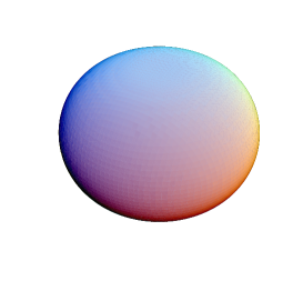
(a)       (b)

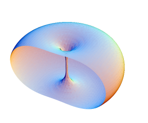
Figure 1: The energy isosurfaces for the charge 1 (a) and the charge 2 (b) static Hopfions at $\mu^{2}=2$ and $\omega=0$.

The resulting system of the Euler-Lagrange equations can be solved when we impose the boundary conditions such that the resulting field configuration will be regular on the symmetry axis, at the origin and on the spatial asymptotic.

The charge $Q=1$ ${\cal A}_{1,1}$ configuration possesses the maximum of the energy density at the origin, the energy density isosurfaces are squashed spheres as seen in Fig.1, left. The charge $Q=2$ ${\cal A}_{2,1}$ solutions have toroidal structure( see Fig.1, right). Inclusion of the mass term increases the attraction in the system, the total energy of the massive Hopfion increases monotonically as mass parameter $\mu$ increases [21].

The residual $O(2)$ global symmetry of the ansatz (2) with respect to the rotations around the third axis in the internal space allows us to consider the stationary spinning classical Hopfions

$$\phi_{+}\to\phi_{+}\mathrm{e}^{\mathrm{i}\omega t};\qquad\phi_{-}\to\phi_{-}\mathrm{e}^{-\mathrm{i}\omega t}$$ (4)

Here, to secure stability of the configuration with respect to radiation, the rotation frequency $\omega$ is a parameter restricted to the interval

$$0\leq\omega<\mu$$ (5)

Substituting this ansatz into the lagrangian (1) gives

$$L=-M+\frac{\omega^{2}\Lambda}{2}$$ (6)

where $M$ is the static energy of the Hopfion and $\Lambda$ is the moment of inertia

$$\Lambda=\frac{1}{16\pi}\int\sin\theta\mathrm{d}r\mathrm{d}\theta\biggl{[}\sin^{2}f\biggl{(}2r^{2}+\Bigl{(}\frac{\partial f}{\partial\theta}\Bigr{)}^{2}+r^{2}\Bigl{(}\frac{\partial f}{\partial r}\Bigr{)}^{2}\biggr{)}\biggr{]}\,,$$ (7)

and the conserved quantity is the classical spin of the rotating configuration $J=\omega\Lambda$.

Note that the structure of the expression for the density of the moment of inertia (7) in the rigid body approximation does not depend on the phase function $g(r,\theta)$. However the function $f(r,\theta)$ is angle dependent.

The mass of the static Hopfion as a function of the parameter $\mu$ is presented in Fig. 2, as $\mu=0$ the corresponding values of the Hopfion mass and the moment of inertia are $M_{Q=1}=1.23,\leavevmode\nobreak\ \leavevmode\nobreak\ \Lambda_{Q=1}=0.63$ and $M_{Q=2}=1.97,\leavevmode\nobreak\ \leavevmode\nobreak\ \Lambda_{Q=2}=0.41$

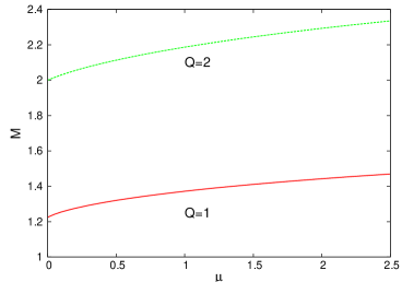
Figure 2: The static energy of the axially-symmetric ${\cal A}_{1,1},{\cal A}_{2,1}$ Hopfions as function of the mass parameter $\mu$ at $\omega=0$.

As the angular velocity $\omega$ increases, the total energy of the spinning configuration as well as the moment of inertia and the angular momentum are increasing monotonically [18]. Investigation of the energy density distribution reveal very interesting picture, as $\omega$ increases a hollow circular tube is formed inside the Hopfion energy shell, both for the charge 1 and charge 2 as shown in Figs.3. The moment of inertia of the configuration diverges as $\omega\to\mu$.

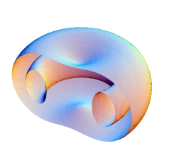
(a)       (b)

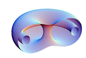
Figure 3: The energy isosurfaces of the ${\cal A}_{1,1}$ (a) and the ${\cal A}_{2,1}$ (b) spinning Hopfions at $\omega^{2}\sim\mu^{2}=2$.

The classical spinning Hopfion can be quantized within the Bohr-Sommerfield scheme by requiring the spin to be quantized as $J^{2}=j(j+1)$, where $j$ is the rotational quantum number taking half-integer values [4, 22]. The difference between our approach, where rotation occurs only around $z$ axis and therefore is characterized by of U(1) representations (i.e. takes only integer values), and the discussion presented in the paper [22] in that in the latter case the charge $Q=1$ ${\cal A}_{1,1}$ configuration was considered by a analogy with the case of the spinning Skyrmion where the usual hedgehog ansatz $U=\exp\left(\mathrm{i}F(r)(\hat{n}^{a}\cdot\tau_{a})\right)$ with a single radially dependent profile function $f(r)$ was implemented instead of the parametrization (2). The relation between these two parametrizations can be explicitly written as

$$\phi_{+} = \sqrt{2}\sin F(r)\sin\theta\mathrm{e}^{-\mathrm{i}\varphi}\Bigl{(}\sin F(r)\cos\theta-\mathrm{i}\cos F(r)\Bigr{)},$$

$$\phi_{0} = \cos(2\theta)\sin^{2}F(r)+\cos^{2}F(r),$$

$$\phi_{-} = -\sqrt{2}\sin F(r)\sin\theta\mathrm{e}^{\mathrm{i}\varphi}\Bigl{(}\sin F(r)\cos\theta+\mathrm{i}\cos F(r)\Bigr{)}$$ (8)

The functions $f(r,\theta)$ and $g(r,\theta)$ which parametrize the axially-symmetric ansatz (2) are related to the approximation by radial function $F(r)$ of [22] as

$$\cos f(r,\theta) = \cos(2\theta)\sin^{2}F(r)+\cos^{2}F(r),$$ (9)

$$\tan g(r,\theta) = \frac{\cos F(r)}{\sin F(r)\cos\theta}.$$ (10)

Surprisingly, the hedgehog parametrization works extremely well for the minimal energy ${\cal A}_{1,1}$ configuration. It was pointed out also by Ward [23] who used the stereographic parametrization of the ${\cal A}_{1,1}$ and ${\cal A}_{2,1}$ Hopfions in terms of the single radial-dependent function ${\cal F}(r)$. For the former case this parametrisation is:

$$W=\frac{x+\mathrm{i}y}{z-\mathrm{i}{\cal{F}}}=\frac{\sin\theta}{\sqrt{\cos^{2}\theta+\frac{{\cal{F}}^{2}}{r^{2}}}}\mathrm{e}^{\mathrm{i}\bigl{(}\varphi+\mathrm{arctg}\frac{{\cal{F}}}{r\cos\theta}\bigr{)}}$$ (11)

The relation to the ansatz (2) is given by the expression

$$\phi_{a}=\frac{\sqrt{2}}{1+|W|^{2}}\bigl{(}-W,\frac{1}{\sqrt{2}}(1-|W|^{2}),\bar{W}\bigr{)}\,,$$ (12)

thus, we can represent the profile functions $f(r,\theta)$ and $g(r,\theta)$ as

$$\cos f(r,\theta) = \frac{r^{2}\cos 2\theta+{\cal{F}}^{2}}{r^{2}+{\cal{F}}^{2}},$$ (13)

$$\mathop{\mathrm{tg}}\,g(r,\theta) = -\frac{{\cal{F}}}{r\cos\theta}.$$ (14)

Finally, note that these two radial functions $F(r)$ and ${\cal F}(r)$ which are used in the parametrizations (2) and (11), respectively, are related as

$${\cal{F}}=-2\mathop{\mathrm{ctg}}\,F(r)$$ (15)

Thus we will revisit the problem of the canonical quantization of the Hopfion using approach previously discussed in [15]-[17]. For the sake of simplicity here we restrict our analyse to the case of the axially-symmetric configurations ${\cal A}_{1,1},{\cal A}_{2,1}$.

Similarity of the Lagrangian (1) with the conventional Skyrme model suggests that in order to apply the standard canonical quantization procedure it is convenient to re-express the expression (1) in terms of the hermitian matrix fields

$$H=\left(\begin{array}[]{ll}\cos f(r,\theta)&\sin f(r,\theta)\mathrm{e}^{-\mathrm{i}(n\varphi-mg(r,\theta))}\\ \sin f(r,\theta)\mathrm{e}^{\mathrm{i}(n\varphi-mg(r,\theta))}&-\cos f(r,\theta)\end{array}\right).$$ (16)

which parametrises the Hopfion configuration. This matrix can be written compactly as

$$H=2\sum_{a}(-1)^{a}\tau_{a}\phi_{-a};\qquad H\cdot H=\mathbf{1}$$ (17)

where the usual algebra of the Pauli matrices $(\tau_{+},\tau_{0},\tau_{-})$ yields

$$\tau_{a}\tau_{b}=\frac{1}{4}(-1)^{a}\delta_{a,-b}\mathbf{1}-\frac{1}{\sqrt{2}}\left[\begin{matrix}1&1&1\\ a&b&c\end{matrix}\right]\tau_{c}.$$ (18)

Here the symbol in the square brackets is the $SU(2)$ Clebsh-Gordan coefficient.

In this notations the Lagrangian (1) can be rewritten as (the metric $\mathop{\mathrm{diag}}(1,-1,-1,-1)$ is explicitly assumed).

$${\cal L}=\frac{1}{64\pi^{2}}\left(\mathop{\mathrm{Tr}}\partial_{\mu}H\partial^{\mu}H+\frac{\kappa}{16}\mathop{\mathrm{Tr}}\bigl{[}\partial_{\mu}H,\partial_{\nu}H\bigr{]}\bigl{[}\partial^{\mu}H,\partial^{\nu}H\bigr{]}-\frac{\mu^{2}}{2}\mathop{\mathrm{Tr}}\bigl{(}\mathbf{1}-4\tau_{0}H\tau_{0}H\bigr{)}\right).$$ (19)

3 Quantization. Momenta of inertia

Similarity of the form of the Lagrangian (19) with that of the Skyrme model suggests that we can quantize the rotational degrees of freedom of the axially-symmetric Hopfion by wrapping the ansatz (16) with time-dependent unitary matrices $\mathbf{A}\bigl{(}q(t)\bigr{)}$ [12] which rotates the configuration about the third axis:

$$\mathbf{U}(q,f,g)=\mathbf{A}\bigl{(}q(t)\bigr{)}H\mathbf{A}^{\dagger}\bigl{(}q(t)\bigr{)}.$$ (20)

Thereafter the collective rotational degrees of freedom $q(t)$ are treated as quantum-mechanical variables, i.e. the generalized rotational coordinate $q(t)$ and velocity $\dot{q}(t)$ satisfy the commutation relations

$$\bigl{[}\dot{q},q\bigr{]}=\mathrm{i}f_{00}\,.$$ (21)

The explicit form of the constant $f_{00}$ will be completely determined by canonical commutation relations between quantum coordinates and momenta. As usual, to calculate the effective Lagrangian of the rotational zero mode we have to evaluate the time derivative of the matrix

$$\dot{}\mathbf{U}=\dot{}\mathbf{A}H\mathbf{A}^{\dagger}-\mathbf{A}H\mathbf{A}^{\dagger}\dot{}\mathbf{A}\mathbf{A}^{\dagger},$$ (22)

$$\nabla_{k}U=\mathbf{A}\nabla_{k}H\mathbf{A}^{\dagger}$$ (23)

Taking into account the commutation relation (21) we obtain

$$\mathbf{A}(q)=\exp\bigl{(}\mathrm{i}q\tau_{0}\bigr{)};\qquad\mathbf{A}^{\dagger}\dot{}\mathbf{A}=\mathrm{i}\tau_{0}\dot{q}+\frac{\mathrm{i}}{8}f_{00}\mathbf{1}.$$ (24)

Then, keeping only terms proportional to the square of the angular velocity the effective kinetic Lagrangian density can be written as

$$\mathcal{L}_{q}\approx\frac{\sin^{2}f}{64\pi^{2}r^{2}}\dot{q}^{2}\biggl{(}2r^{2}+\Bigl{(}\frac{\partial f}{\partial\theta}\Bigr{)}^{2}+r^{2}\Bigl{(}\frac{\partial f}{\partial r}\Bigr{)}^{2}\biggr{)}\equiv\frac{1}{2}\dot{q}^{2}\leavevmode\nobreak\ g_{00}\,.$$ (25)

Utilizing the definition of the moment of inertia (7) we can write

$$L_{q}=\frac{1}{2}\dot{q}^{2}\int\mathrm{d}^{3}rg_{00}=\frac{1}{2}\dot{q}^{2}\Lambda$$ (26)

Thought the expression (26) coincides with its classical counterpart in (6), the corresponding quantum momentum is conjugated to the rotational collective coordinate $q$ and it is defined as

$$\hat{p}=\frac{\partial L_{q}}{\partial\dot{q}}=\Lambda\dot{q}$$ (27)

Thus, the canonical commutation relation $\bigl{[}\hat{p},q\bigr{]}=-\mathrm{i}$ allows us to define $f_{00}=\frac{1}{\Lambda}$. We can also define the U(1) group generator which is the angular momentum operator

$$\hat{}\mathbf{J}=-\hat{p}=-\Lambda\dot{q}$$ (28)

for eigenstates $|k\rangle=\mathrm{e}^{-\mathrm{i}kq}|0\rangle$ with integer eigenvalues $k=0,\pm 1,\pm 2,\ldots$.

We are now in position to evaluate the explicit form of the quantum-mechanical Lagrangian of the Faddeev-Skyrme model. Using expression (24) we obtain:

$$\begin{split}\mathcal{L}_{q}&=\frac{1}{64\pi^{2}}\biggl{(}\mathop{\mathrm{Tr}}\dot{}\mathbf{U}\dot{}\mathbf{U}-\frac{1}{8}(-1)^{a}\mathop{\mathrm{Tr}}\mathbf{A}\bigl{[}\bigl{[}\mathbf{A}^{\dagger}\dot{}\mathbf{A},H\bigr{]},\nabla_{a}H\bigr{]}\bigl{[}\bigl{[}\mathbf{A}^{\dagger}\dot{}\mathbf{A},H\bigr{]},\nabla_{-a}H\bigr{]}\mathbf{A}^{\dagger}\biggr{)}\\ &=\frac{\sin^{2}f}{64\pi^{2}}\left(\dot{q}^{2}+\frac{1}{4\Lambda^{2}}\right)\biggl{(}2+\frac{1}{r^{2}}\biggl{(}\Bigl{(}\frac{\partial f}{\partial\theta}\Bigr{)}^{2}+\Bigl{(}\frac{\partial f}{\partial r}\Bigr{)}^{2}\biggl{)}\biggl{)}\\ &=\frac{\sin^{2}f}{64\pi^{2}\Lambda^{2}}\left(\hat{}\mathbf{J}^{2}+\frac{1}{4}\right)\biggl{(}2+\frac{1}{r^{2}}\biggl{(}\Bigl{(}\frac{\partial f}{\partial\theta}\Bigr{)}^{2}+\Bigl{(}\frac{\partial f}{\partial r}\Bigr{)}^{2}\biggl{)}\biggl{)}\end{split}$$ (29)

The total effective Hamiltonian corresponds to the complete Lagrangian $L=L_{\mathrm{cl}}+L_{q}$which includes both classical and quantum mechanical parts:

$$H=\frac{1}{2}\bigl{\{}\hat{p},\dot{q}\bigr{\}}-L=\frac{\hat{}\mathbf{J}^{2}}{2\Lambda}-L_{\mathrm{cl}}+\Delta M$$ (30)

Here the quantum mass correction $\Delta M$ appears when the canonical commutation relation is taken into account:

$$\Delta M=-\frac{1}{8\cdot 16\pi\Lambda^{2}}\int\sin\theta\mathrm{d}r\mathrm{d}\theta\biggl{[}\sin^{2}f\biggl{(}2r^{2}+\Bigl{(}\frac{\partial f}{\partial\theta}\Bigr{)}^{2}+r^{2}\Bigl{(}\frac{\partial f}{\partial r}\Bigr{)}^{2}\biggr{)}\biggr{]}=-\frac{1}{8\Lambda}$$ (31)

where we used the definition (7). Note that an interesting peculiarity of the integrand in (31) is that it exactly reproduces the structure of the density of the moment of inertia (7), thus in the rigid body approximation we can immediately evaluate the quantum corrections to the axially-symmetric configurations ${\cal A}_{1,1},{\cal A}_{2,1}$ as

$$\Delta M_{1,1}=-\frac{1}{8\Lambda_{Q=1}}=-0.20;\qquad\Delta M_{2,1}=-\frac{1}{8\Lambda_{Q=2}}=-0.30$$ (32)

thus, for the configurations with topological charges $Q=1,2$ the quantum correction to the Hopfion mass is negative and it is about $16\%$ and $25\%$ of the classical masses, respectively.

A more consistent treatment of the quantum correction to the Hopfion mass needs minimization of the total energy functional

$$\begin{split}\mathcal{H}=-\mathcal{L}_{\mathrm{cl}}+\frac{\sin^{2}f}{32\pi^{2}r^{2}}\Bigl{(}\frac{\hat{}\mathbf{J}^{2}}{2\Lambda^{2}}-\frac{1}{8\Lambda^{2}}\Bigr{)}\biggl{(}2r^{2}+\Bigl{(}\frac{\partial f}{\partial\theta}\Bigr{)}^{2}+r^{2}\Bigl{(}\frac{\partial f}{\partial r}\Bigr{)}^{2}\biggl{)}\end{split}$$ (33)

Varying it we obtain rather cumbersome set of two coupled integro-differential equation for functions $f(r,\theta)$ and $g(r,\theta)$ which then should be solved numerically. The results will be reported elsewhere.

Conclusion

The main purpose of this letter was to present the scheme of the canonical quantization of the rotational mode of the charge $Q=1$ and $Q=2$ spinning Hopfions and evaluate the quantum corretions to the mass of these axially-symmetric configurations. To this end we have used the technique described in [15]-[17] in the context of the Skyrme model and Baby Skyrme model [24]. The model is stabilised by additional coupling to a potential (mass) term by analogy with the Baby Skyrme model, this leads to appearance of the Yukawa-type exponential tail of the Hopfion fields. The analysis of the quantum corrections to the mass of the axially symmetric charge $Q=1,2$ solitons showed that, like in the Skyrme model, the corrections are negative and relatively large.

It remains to systematically analyze the effect of quantization of the rotating Hopfions beyond the usual Bohr -Sommerfeld framework and the rigid body approximation we implemented in the present letter. As a direction for future work, it would be interesting to study the effect of canonical quantisations of the spinning knotted Hopfions, e.g. to consider how the shape of the celebrated $Q=7$ trefoil knot configuration ${\cal K}_{3,2}$ will be affected by the quantum corrections or if the axial symmetry of the spinning charge $Q=3$ buckled configuration will be restored. Other buckling and twisting transmutations of the Hopfions which are related with a change of the symmetry of various spinning configurations of higher Hopf degree are also possible, one can expect an axially symmetric state may be the lowest energy state in this case. This work is now in progress [18].

References

- [1] T. H. R. Skyrme, Proc. Roy. Soc. Lond. A 260 (1961) 127.
-
[2]
G. ‘t Hooft, Nucl. Phys. B 79 (1974) 276;
A.M. Polyakov, Pis’ma JETP 20 (1974) 430. -
[3]
L.D. Faddeev, Quantization of Solitons, ,
Preprint-75-0570, IAS, Princeton (1975);
L.D Faddeev and A. Niemi, Nature 387, 58 (1997); Phys. Rev. Lett. 82, 1624 (1999). - [4] J. Gladikowski and M. Hellmund, Phys. Rev. D 56 (1997) 5194 [arXiv:hep-th/9609035].
- [5] R. Battye and P. Sutcliffe, Phys. Rev. Lett. 81 4798 (1998)
- [6] J. Hietarinta and P. Salo, Phys. Rev. D 62, 081701 (2000).
- [7] P. Sutcliffe, Proc. Roy. Soc. Lond. A 463 (2007) 3001 [arXiv:0705.1468 [hep-th]].
- [8] E. Babaev, L.D. Faddeev and A.J. Niemi, Phys. Rev. B 65, 100512(R) (2002); J. Jÿkkä and J. Hietarinta, Phys. Rev. B 77, 094509 (2008)
-
[9]
W. S. Bae, Y. M. Cho and S. W. Kim,
Phys. Rev. D 65, 025005 (2002);
K. -I. Kondo, A. Ono, A. Shibata, T. Shinohara and T. Murakami, J. Phys. A A 39, 13767 (2006) [hep-th/0604006]. - [10] G.S. Adkins, C.R. Nappi and E. Witten, Nucl. Phys. B 228 (1983) 552.
- [11] G. S. Adkins and C. R. Nappi, Nucl. Phys. B 233 (1984) 109.
- [12] G. S. Adkins, C. R. Nappi and E. Witten, Nucl. Phys. B 228 (1983) 552.
- [13] R. A. Battye, S. Krusch and P. M. Sutcliffe, Phys. Lett. B 626 (2005) 120 [arXiv:hep-th/0507279].
- [14] K. Fujii, K. I. Sato, N. Toyota and A. P. Kobushkin, Phys. Rev. Lett. 58 (1987) 651.
- [15] K. Fujii, A. Kobushkin, K. I. Sato and N. Toyota, Phys. Rev. D 35, 1896 (1987).
- [16] A. Acus, E. Norvaisas and D. O. Riska, Nucl. Phys. A 614 (1997) 361 [arXiv:hep-ph/9605435].
- [17] D. Jurciukonis, E. Norvaisas and D. O. Riska, J. Math. Phys. 46 (2005) 072103 [arXiv:nucl-th/0505003].
- [18] J. Jäykkä, D. Harland, J.M. Speight and Ya. Shnir, work in progress.
- [19] A.F. Vakulenko and L.V. Kapitansky, Sov. Phys. Dokl. 24, 432 (1979).
- [20] Ya.M. Shnir and D.H. Tchrakian, J. Phys. A: Math. Theor. 43 (2010) 025401 (11pp); arXiv:0906.5583 [hep-th]
- [21] D. Foster, Phys. Rev. D 83 (2011) 085026 [arXiv:1012.2595 [hep-th]].
- [22] W. C. Su, Phys. Lett. B 525 (2002) 201 [arXiv:hep-th/0108047].
- [23] R. S. Ward, Phys. Lett. B 473 (2000) 291 [arXiv:hep-th/0001017].
- [24] A. Acus, E. Norvaisas and Ya.M. Shnir, Phys. Lett. B 682 (2009) 155.