Replica Cluster Variational Method: the Replica Symmetric solution for the 2D random bond Ising model

Abstract

We present and solve the Replica Symmetric equations in the context of the Replica Cluster Variational Method for the 2D random bond Ising model (including the 2D Edwards-Anderson spin glass model). First we solve a linearized version of these equations to obtain the phase diagrams of the model on the square and triangular lattices. In both cases the spin-glass transition temperatures and the tricritical point estimations improve largely over the Bethe predictions. Moreover, we show that this phase diagram is consistent with the behavior of inference algorithms on single instances of the problem. Finally, we present a method to consistently find approximate solutions to the equations in the glassy phase. The method is applied to the triangular lattice down to $T=0$, also in the presence of an external field.

I Introduction

Since the celebrated work of Edwards and Anderson in 1975 Edwards and Anderson (1975) many efforts have been devoted to the analytic description of spin glasses. Very remarkable is the solution found by Parisi in 1979 Parisi (1979, 1980) to the Sherrington-Kirkpatrick mean-field model Kirkpatrick and Sherrington (1978). The physical interpretation of the Parisi solution Parisi et al. (1987) gave a solid basis to concepts like Replica Symmetry (RS) and spontaneous Replica Symmetry Breaking (RSB), that became of standard use in the scientific community. The solutions of many models, not necessarily of mean field type, were interpreted along these ideas (see e.g. the review in Marinari et al. (2000) about spin glasses on finite dimensional lattices).

In this context the last decade has been very exciting both from the conceptual and from the practical point of view. First, Mézard and Parisi Mézard and Parisi (2001, 2003) were able to solve analytically the spin glass model on a Bethe lattice (usually called the Viana-Bray model Viana and Bray (1985)) with a Replica Symmetry Breaking ansatz. Within this RSB ansatz, the solution is given in terms of populations of fields that contain all the necessary information to describe the low temperature phase of the model. The extension to other models was immediate Mezard et al. (2002); Mézard and Zecchina (2002); Mulet et al. (2002) and the approach was fundamental to the introduction of the Survey Propagation algorithm Mézard and Zecchina (2002) that has been successfully applied in the solution of many single instances optimization problems Braunstein et al. (2003); Zhou (2003). Moreover it was soon recognized that the well-known Belief Propagation (BP) algorithm Pearl (1988) corresponds to the Bethe approximation Kabashima and Saad (1998), that is the replica symmetric solution on the Bethe lattice.

Unfortunately all the above analytical results concern mean-field models. To go beyond the Bethe approximation, one should consider also loops in the interaction network and this turns out to be a highly non trivial task (see for example Montanari and Rizzo (2005); Chertkov and Chernyak (2006, 2006); Mooij and Kappen (2007); Gomez et al. (2010); Xiao and Zhou (2011)). Yedidia and coworkers Yedidia et al. (2005) described how to generalize the Cluster Variational Method (CVM) of Kikuchi Kikuchi (1951) that allows to derive a free-energy that improves the Bethe one by considering exactly the contribution of small loops. The minimization of the CVM free energy can be achieved by the use of a Generalized Belief Propagation (GBP) algorithm Yedidia et al. (2005), but the solution found is always replica symmetric.

The idea of merging the CVM with the RSB ansatz was around for some years, but it remained elusive. Probably because the simplest comprehension of the RSB ansatz within the Bethe approximation is based on a probabilistic cavity construction Mézard and Parisi (2001), which is hard (or even impossible) to derive for a general CVM. In a recent paper Rizzo et al. (2010) we proposed a formal solution to this problem. The idea was to apply the CVM to an already replicated free energy, and then within the RSB ansatz to send the number of replicas to zero. This formulation allowed us to derive a set of closed equations for some local fields, that play the same role of the cavity fields in the Bethe approximation. Unfortunately these fields enter into the equations in an implicit form and so standard population dynamic algorithms can not be used for finding the solution. In previous works Rizzo et al. (2010); Domínguez et al. (2011), using linear stability analysis, we showed that these equations improve the Bethe approximation on the location of the phase boundaries. However the solution of these equations in the low temperature phase, and the interpretation of this solution in terms of the performance of inference algorithms are still important open problems.

The main goal of this work is to extend our previous results in these two directions. On the one hand, using a stability analysis we study the phase diagram in the $\rho$ (density of ferromagnetic couplings) versus $T$ (temperature) plane for the Edwards-Anderson model on the square and triangular lattices. Moreover, we show that the Generalized Belief Propagation algorithm (GBP) stops converging close to the spin-glass temperature predicted by our approximation. On the other hand, we propose an approximated method to deal, at the RS level, with the complex equations that arise in the formalism in the low $T$ phase.

The rest of the work is organized as follows. In the next section, we rederive the equations already obtained in Rizzo et al. (2010) but now limiting its scope to the RS scenario in the average case. In section III we present the phase diagram obtained by a linearized version of these equations and in IV we study the consequences of this phase diagram for the perfomance of GBP. Section V show the solution of a non-linear approximation for the RS equations in the glassy phase. Finally, the conclusions and possible extensions of our approach are outlined in section VI.

II The CVM Replica Symmetric solution

The Edwards-Anderson model is defined by the Hamiltonian $H=-\sum_{(ij)}J_{ij}s_{i}s_{j}-h\sum_{i}s_{i}$, where the first sum is over neighboring spins on a finite dimensional lattice, the couplings $J_{ij}$ are quenched random variables and $h$ is the external field. Although the equations we write are valid for generic couplings, our results will be obtained for couplings drawn from the distribution $P(J)=\rho\,\delta(J-1)+(1-\rho)\delta(J+1)$.

In a model with quenched disorder the free-energy of typical samples can be obtained from the $n\to 0$ limit of the replicated free-energy

$$\Phi(n)=-{1\over n\beta\,N}\ln{\rm Tr}\left\langle\exp\Big{(}\sum_{(ij)}\beta J_{ij}\sum_{a=1}^{n}s_{i}^{a}s_{j}^{a}+\sum_{i}\beta h\sum_{a=1}^{n}s_{i}^{a}\Big{)}\right\rangle_{J}=\\ =-{1\over n\beta\,N}\ln{\rm Tr}\exp\left(\sum_{(ij)}\ln\Big{\langle}\exp\beta J\sum_{a}s_{i}^{a}s_{j}^{a}\Big{\rangle}_{J}+\sum_{i}\beta h\sum_{a=1}^{n}s_{i}^{a}\right)\;,$$ (1)

where $n$ copies of a system of $N$ spins are considered at inverse temperature $\beta$, and the average over the quenched disorder is represented by the angular brackets.

The starting point of the Kikuchi’s CVM approximation is to choose a set of regions of the graph over which the model is defined. Restricting only to link and node regions, the cluster variation method recovers Bethe approximation. We will concentrate here on three kind of regions: plaquettes (square or triangles, depending on the lattice), links and nodes. Using the definition, $\psi_{r}(\sigma_{r})\equiv\prod_{i,j\in r}\langle\exp\beta J\sum_{a}s_{i}^{a}s_{j}^{a}\rangle_{J}$ the energy of region $r$ is:

$$E_{r}=-\ln\prod_{ij}\psi_{ij}(\sigma_{i},\sigma_{j})-\ln\prod_{i}\psi_{i}(\sigma_{i})\;,$$ (2)

where the products run over all links and nodes (in presence of a field) contained in region $r$. Let us also define the belief $b_{r}(\sigma_{r})$ as an estimation of the marginal probability of the configuration $\sigma_{r}$ according to the Gibbs measure. Then, within this approximation, the Kikuchi’s free energy takes the form:

$$F_{K}=\sum_{r\in R}c_{r}\left(\sum_{x_{r}}b_{r}E_{r}+\sum_{x_{r}}b_{r}\ln b_{r}\right)\;,$$ (3)

where the so-called Moebius coefficient $c_{r}$ is the over-counting number of region $r$ Yedidia et al. (2005). In the case of the EA in the square lattice, the biggest regions are the square plaquettes, and by definition $c_{P}=1$. Since each link region is contained in two plaquettes, $c_{L}=1-2=-1$. Moreover, the spins regions are contained in 4 plaquettes and 4 links and $c_{S}=1-4\cdot c_{P}-4\cdot c_{L}=1$. Similarly for the triangular lattices $c_{P}=1$, $c_{L}=1-2\cdot c_{P}=-1$ and $c_{S}=1-6\cdot c_{P}-6\cdot c_{L}=1$.

Now, the Kikuchi free energy has to be extremized with respect to the beliefs $b_{r}(\sigma_{r})$, subject to the constraint that they are compatible upon marginalization. For example, $b_{(ij)}(\sigma_{i},\sigma_{j})=\sum_{\sigma_{k},\sigma_{l}}b_{(ijkl)}(\sigma_{i},\sigma_{j},\sigma_{k},\sigma_{l})$ and $b_{i}(\sigma_{i})=\sum_{\sigma_{j}}b_{(ij)}(\sigma_{i},\sigma_{j})$ for the square lattice. It is already a standard procedure Yedidia et al. (2005); Pelizzola (2005) to show that under these conditions the beliefs can be written as:

$$b_{r}(\sigma_{r})\propto\psi_{r}(\sigma_{r})\prod_{(r^{\prime},s^{\prime})\in M(r)}m_{r^{\prime}s^{\prime}}(\sigma_{r})\;,$$ (4)

where $M(r)$ is the set of connected pairs of regions $(r^{\prime},s^{\prime})$ such that $r^{\prime}\setminus s^{\prime}$ is outside $r$ while $s^{\prime}$ coincides either with $r$ or with one of its subsets (descendants). For example, if $r$ is one link in a square lattice, the product in (4) contains the so-called messages $m$ from the two squares adjacent to it, and the messages $m$ from the six other links connected to it (three on each extreme). The messages $m_{rs}$ obey the following equations:

$$m_{rs}(\sigma_{s})\prod_{(r^{\prime},s^{\prime})\in M(r,s)}m_{r^{\prime}s^{\prime}}(\sigma_{s})\propto\sum_{\sigma_{r\setminus s}}\psi_{r\setminus s}(\sigma_{r})\prod_{(r^{\prime\prime},s^{\prime\prime})\in M(r)\setminus M(s)}m_{r^{\prime\prime}s^{\prime\prime}}(\sigma_{r})\;,$$ (5)

where $M(r,s)$ is the set of connected pairs of regions $(r^{\prime},s^{\prime})$ such that $r^{\prime}$ is a descendant of $r$ and $s^{\prime}$ is either region $s$ or a descendant of $s$.

For the particular cases we are considering here (2D square and triangular lattices) the general expression (5) translates into the following two couple equations. The first equation is identical for both lattices and reads

$$m_{(ij)\rightarrow j}(\sigma_{j})\propto\sum_{\sigma_{i}}\psi_{(ij)}(\sigma_{i},\sigma_{j})M_{\alpha\rightarrow(ij)}(\sigma_{i},\sigma_{j})M_{\beta\rightarrow(ij)}(\sigma_{i},\sigma_{j})\prod_{k\in\partial i\setminus j}m_{(ki)\rightarrow i}(\sigma_{i})\;,$$ (6)

where $\alpha$ and $\beta$ are the two plaquette sharing the link $(ij)$ and $\partial i$ is the set of neighbors of site $i$. The notation used in this equation should make clear that messages are sent between a region and one of its descendant. The second equation takes slightly different forms for the square and triangular lattices, and we write it explicitly for the triangular lattice:

$$M_{(ijk)\to(ij)}(\sigma_{i},\sigma_{j})m_{(ik)\to i}(\sigma_{i})m_{(jk)\to j}(\sigma_{j})\propto\sum_{\sigma_{k}}\psi_{(ik)}(\sigma_{i},\sigma_{k})\psi_{(jk)}(\sigma_{j},\sigma_{k})\\ \prod_{\alpha\in\partial(ik)\setminus(ijk)}M_{\alpha\to(ik)}(\sigma_{i},\sigma_{k})\prod_{\beta\in\partial(jk)\setminus(ijk)}M_{\beta\to(jk)}(\sigma_{j},\sigma_{k})\prod_{l\in\partial k\setminus\{i,j\}}m_{l\to k}(\sigma_{k})\;,$$ (7)

where, in practice, the first two products only contain one message each. For the square lattice the equation modifies slightly and contains some more products; disregarding all indices and arguments, its schematic form is $M\,m\,m\propto\sum\psi\,\psi\,\psi\prod M\prod M\prod M\prod m\prod m$.

Up to this point the only difference with the standard CVM method is the introduction of replicated spins $\sigma_{i}$ and the non obvious connection with the average over the disorder, implicitly introduced in $\psi_{r}(\sigma_{r})$. The main contribution of our previous work Rizzo et al. (2010) was to introduce a consistent scheme to write these equations in the limit $n\rightarrow 0$ at any level of RSB.

Here we reproduce the approach for the average case at the RS level. Following Monasson (1998), we start by parametrizing the link to node messages in the following way:

$$m(\sigma_{i})=\int du\,q(u)\exp\left[\beta u\sum_{a=1}^{n}\sigma_{i}^{a}\right](2\cosh\beta u)^{-n}\;,$$ (8)

and extend the same idea to the parametrization of the plaquette to link messages:

$$M(\sigma_{i},\sigma_{j})\propto\int dU\,du_{i}\,du_{j}\,Q(U,u_{i},u_{j})\exp\left[\beta U\sum_{a=1}^{n}\sigma_{i}^{a}\sigma_{j}^{a}+\beta u_{i}\sum_{a=1}^{n}\sigma_{i}^{a}+\beta u_{j}\sum_{a=1}^{n}\sigma_{j}^{a}\right]\;.$$ (9)

The above parametrization allows to rewrite the message passing equations (5) in terms of $q(u)$ and $Q(U,u_{1},u_{2})$. Substituting equations (8) and (9) into (6) and (7) and sending $n\rightarrow 0$, we obtain, after some standard algebra,

$$q(u) = \int\prod_{i}^{k}dq_{i}\prod_{\alpha}^{p}dQ_{\alpha}\,\langle\delta(u-\hat{u}(\#))\rangle_{J}\;,$$

$$R(U,u_{a},u_{b}) \equiv \int du_{i}\,du_{j}\,Q(U,u_{i},u_{j})q(u_{a}-u_{i})q(u_{b}-u_{j})=$$

$$= \int\prod_{i}^{K}dq_{i}\prod_{\alpha}^{P}dQ_{\alpha}\,\langle\delta(U-\hat{U}(\#))\delta(u_{a}-\hat{u}_{a}(\#))\delta(u_{b}-\hat{u}_{b}(\#))\rangle_{J}\;,$$

where $k$ ($p$) and $K$ ($P$) correspond to the number of small $m$ (large $M$) messages that enter into each equation. The specific expressions for $\hat{u}(\#),\hat{U}(\#),\hat{u}_{a}(\#),\hat{u}_{b}(\#)$ depend on the lattice. The expressions for the triangular lattices are given in the next section and we refer the reader to reference Lage-Castellanos et al. (2011) for similar formulas for the square lattice.

The next step is to solve the self-consistency equations in (II). Then, once $q$ and $Q$ are known, the thermodynamical observables are well defined in term of these objects Rizzo et al. (2010). Unfortunately, since in (II) the functions $Q$ and $q$ are convoluted, this problem can not be straightforwardly approached using standard population dynamics algorithm. One possible approach is to deconvolve $R$ using Fourier techniques to extract $Q$. Unfortunately, this approach suffers from strong instability problems. To use any numerical Fourier transform, one must have $R$ and $Q$ in form of histograms. But since $Q$ is not necessarily positive defined Rizzo et al. (2010) the sampling of the messages becomes hard and the numerical errors due to the discretization of $Q$ combine with the errors due to the Fourier inversion process making difficult the convergence at low temperatures. To bypass these numerical problems we choose to solve these equations approximately. We perturb them in terms of small parameters around the paramagnetic solution and keep track of the information about the first few moments of the distributions.

III Phase Diagram from the linearized equations

Since the exact computation of $q(u)$ and $Q(U,u_{1},u_{2})$ is a daunting task, here we concentrate our attention on the calculation of their first two moments:

$$m=\int q(u)\,u\,\mathrm{d}u\;,\qquad a=\int q(u)\,u^{2}\mathrm{d}u\;,\qquad a_{0}(U)=\iint Q(U,u_{1},u_{2})\,\mathrm{d}u_{1}\,\mathrm{d}u_{2}\;,$$

$$M_{i}(U)=\iint Q(U,u_{1},u_{2})\,u_{i}\,\mathrm{d}u_{i}\;,\qquad a_{ij}(U)=\iint Q(U,u_{1},u_{2})\,u_{i}\,u_{j}\,\mathrm{d}u_{1}\mathrm{d}u_{2}\;,$$ (11)

where $i,j\in\{1,2\}$. With these definitions the moments are determined by

$$m = \int\prod_{i}^{k}dq_{i}\prod_{\alpha}^{p}dQ_{\alpha}\langle\hat{u}\rangle_{J}$$ (12)

$$a = \int\prod_{i}^{k}dq_{i}\prod_{\alpha}^{p}dQ_{\alpha}\langle\hat{u}^{2}\rangle_{J}$$

$$M_{1}(U) = \int du_{1}du_{2}R(U,u_{1},u_{2})\langle u_{1}\rangle_{J}-m\,a_{0}(U)$$

$$a_{11}(U) = \int du_{1}du_{2}R(U,u_{1},u_{2})\langle u_{1}^{2}\rangle_{J}-2mM_{1}(U)-a\,a_{0}(U)$$

$$a_{12}(U) = \int du_{1}du_{2}R(U,u_{1},u_{2})\langle u_{1}u_{2}\rangle_{J}-2mM_{1}(U)-m^{2}a_{0}(U)$$

However, keep in mind that $R(U,u_{1},u_{2})$ is still defined in terms of $q$ and $Q$, see (II), and not directly in terms of the moments. Therefore, in order to compute the integrals in (III), one must introduce some ansatz over these distributions. It is then reasonable to start considering as correct the high temperature solution and to linearize the equations around this solution. At high temperatures and zero external field one may assume that the system is paramagnetic:

$$q(u)=\delta(u)\;,\qquad Q(U,u_{1},u_{2})=a_{0}(U)\delta(u_{1})\delta(u_{2})$$ (13)

In what follow we show, first, the linearization of $\hat{u}(\#)$ and $\hat{u}_{i}(\#)$ for the triangular lattice. Then, as an example, the derivation of the expressions for $m$ and $a$ in (III) and leave for the Appendix the expressions for the moments of $Q$. The algebra associated to the equations for the square lattice is more cumbersome, but is technically equivalent. The interested reader may look for the case when $m=0$ in references Rizzo et al. (2010) and Lage-Castellanos et al. (2011).

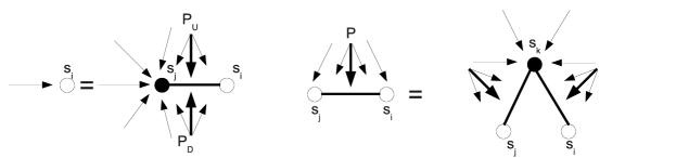
Figure 1: Schematic representation of the message passing equations (II) for the triangular lattice.

To compute $\hat{u}(\#)$ it is enough to understand that the first equation in (II) may be interpreted as a standard equation for the Bethe approximation with a renormalized interaction between the spins $\hat{J}=J+U^{a}+U^{b}$ (see the first panel in Figure 1). Then, one can follow standard calculations Mézard and Montanari (2009) and the expression for the single message $\hat{u}$ reads

$$\hat{u}(\#)=\frac{1}{\beta}\mathrm{arctanh}[\tanh(\beta\hat{J})\tanh(\beta h)]+u_{1}^{a}+u_{1}^{b}\;,$$ (14)

where $u_{1}^{a}$ and $u_{1}^{b}$ are the small messages sent from the corresponding neighbor plaquettes to the site of interest and $h=u_{2}^{a}+u_{2}^{b}+\sum_{i}^{5}u_{i}$ where $u_{2}^{a}$ and $u_{2}^{b}$ are the messages sent from the same plaquettes to the other border of the link. Considering that all the $u$’s and $h$ are small, as must be the case close to the paramagnetic transition, the linearized version of the previous expression becomes

$$\hat{u}(\#)=\tanh(\beta\hat{J})h+u_{1}^{a}+u_{1}^{b}\;.$$ (15)

The messages in the second equation of (II) can be rewritten through the following identities:

$$\hat{U}(\#) = \frac{1}{4\beta}\ln\frac{K(1,1)K(-1,-1)}{K(1,-1)K(-1,1)}$$ (16)

$$\hat{u}_{1}(\#) = \frac{1}{4\beta}\ln\frac{K(1,1)K(1,-1)}{K(-1,1)K(-1,-1)}$$

$$\hat{u}_{2}(\#) = \frac{1}{4\beta}\ln\frac{K(1,1)K(1,1)}{K(1,-1)K(-1,-1)}$$

where $K(S_{1},S_{2})=\sum_{S_{3}}\exp^{\beta\hat{J}_{13}S_{1}S_{3}+\beta\hat{J}_{13}S_{2}S_{3}+u_{1}^{a}S_{1}+u_{1}^{b}S_{2}+h_{3}S_{3}}$ (see the second panel in Figure 1). Then, after some algebra, it is easy to show that

$$\hat{u}_{1}(\#) = \frac{1}{4\beta}\ln\frac{(1+\tanh(\beta J_{+})\tanh(\beta h))(1+\tanh(\beta J_{-})\tanh(\beta h))}{(1+\tanh(\beta J_{+})\tanh(\beta h))(1+\tanh(\beta J_{-})\tanh(\beta h))}$$

$$\sim u_{1}^{a}+\frac{1}{2}h[\tanh(\beta J_{+})+\tanh(\beta J_{-})]$$

and in a similar way

$$\hat{u}_{2}(\#)\sim u_{1}^{b}+\frac{1}{2}h[\tanh(\beta J_{+})-\tanh(\beta J_{-})]\;,$$ (19)

where $J_{+}=(J^{a}+U^{a})+(J^{b}+U^{b})$, $J_{-}=(J^{a}+U^{a})-(J^{b}+U^{b})$ and $h=u_{2}^{a}+u_{2}^{b}+\sum_{i}^{3}u_{i}$. With these expressions we have all the necessary ingredients to write the linearized form of (III). Next, we show how to derive the linear equations for $m$ and $a$ and in the Appendix we present the results for the others.

The single site magnetization $m=\langle u\rangle$ satisfies

$$m=\langle u\rangle=\int duq(u)u=\langle\int dQ_{a}dQ_{b}\prod_{i=1}^{5}dq_{i}u\delta(u-\hat{u}(\#))\rangle_{J}=\langle\int dQ_{a}dQ_{b}\prod_{i=1}^{5}dq_{i}\hat{u}\rangle_{J}=\\ =\langle\int dQ_{a}dQ_{b}\prod_{i=1}^{5}dq_{i}(u_{1}^{a}+u_{1}^{b}+\tanh(\beta\hat{J})h)\rangle_{J}$$ (20)

and using the definitions in (11) the last integral can be easily expressed in linear terms of the moments of the distributions. The result is

$$m=5m\langle\int dU^{a}dU^{b}\tanh(\beta\hat{J})a_{0}(U^{a})a_{0}(U^{b})\rangle_{J}+\int dU^{a}M_{1}(U^{a})+\int dU^{b}M_{1}(U^{b})+\\ +\langle\int dU^{a}dU^{b}\tanh(\beta\hat{J})[a_{0}(U^{b})M_{1}(U^{a})+a_{0}(U^{a})M_{1}(U^{b})]\rangle_{J}$$ (21)

The derivation of $a$ proceeds in a similar way

$$a=\langle u^{2}\rangle=\int duq(u)u^{2}=\langle\int dQ_{a}dQ_{b}\prod_{i=1}^{5}dq_{i}(u_{1}^{a}+u_{1}^{b}+\tanh(\beta\hat{J})h)^{2}\rangle_{J}=\\ \langle\int dQ_{a}dQ_{b}\prod_{i=1}^{5}dq_{i}((u_{1}^{a})^{2}+(u_{1}^{b})^{2}+2u_{1}^{a}u_{1}^{b}+2(u_{1}^{a}+u_{1}^{b})\tanh(\beta\hat{J})+\tanh^{2}(\beta\hat{J})h^{2}\rangle_{J}$$ (22)

that may be re-written in term of the moments:

$$a=\int dU^{a}a_{11}(U^{a})+\int dU^{b}a_{11}(U^{b})+2m\int dU^{a}dU^{b}M_{1}(U^{a})M_{1}(U^{b})+\\ +10m\langle\int dU^{a}dU^{b}\tanh(\beta\hat{J})[a_{0}(U^{a})M_{1}(U^{b})+a_{0}(U^{a})M_{1}(U^{a})]\rangle_{J}+\\ +2\langle\int dU^{a}dU^{b}\tanh(\beta\hat{J})[a_{12}(U^{a})+a_{12}(U^{b})+M_{2}(U^{b})M_{1}(U^{a})+M_{1}(U^{b})M_{2}(U^{a})]\rangle_{J}+\\ +(5a+20m^{2})\langle\int dU^{a}dU^{b}\tanh^{2}(\beta\hat{J})a_{0}(U^{a})a_{0}(U^{b})\rangle_{J}+\\ +10m\langle\int dU^{a}dU^{b}\tanh^{2}(\beta\hat{J})[a_{0}(U^{a})M_{2}(U^{b})+a_{0}(U^{a})M_{2}(U^{a})]\rangle_{J}+\\ +\langle\int dU^{a}dU^{b}\tanh^{2}(\beta\hat{J})[a_{22}(U^{a})+a_{22}(U^{b})+2M_{2}(U^{b})M_{2}(U^{a})]\rangle_{J}$$ (23)

Similar expressions may be derived for $M_{i}$ and $a_{ij}$, see Appendix, but note that they are not closed analytical expressions. The form of $a_{0}(U)$ is unknown, and must be determined for each $\beta$ using population dynamics. Once $a_{0}(U)$ has been computed, one can study the set of linear equations for the moments and check the local stability of the paramagnetic solution. In order to do this, we start from the paramagnetic solution, i.e. all the moments zero, but with $a_{0}(U)$ being non trivial. Then, we slightly perturb $a$ and $m$ and check, solving iteratively Eqs. (21), (23) and (33)-(35) whether these perturbations die out or diverge. Depending on $\rho$ and $T$ we find that under iteration, either both magnitudes diverge, or just $a$ or none. If $a$ and $m$ converge to zero the system is in the paramagnetic phase (P). If only $a$ diverges it is in the spin-glass phase (SG) and if both $a$ and $m$ diverge we say that the system is in a ferromagnetic phase (F).

Figure 2: $\rho$ vs $T$ phase diagram for the square and the triangular lattice. We show results for the Bethe approximation (upper curves) and the Kikuchi approximation (lower curves). It is also shown the Nishimori line (NL). The bold circles on the Nishimori line are the best analytical predictions for the tricritical points. The dashed lines represent the boundaries for the existence of purely ferromagnetic solutions.

The results of this analysis are reported in Figure 2. The phase diagrams must be read in the following way. Below the horizontal lines we have the Spin Glass phase and above the Paramagnetic phase. Critical lines meets at the tricritical point $(\rho^{cr},T^{cr})$, located on the Nishmori line (NL). On the right of this tricritical point, i.e. if $\rho>\rho_{cr}$, the system is in the Ferromagnetic phase at low temperatures and in the Paramagnetic phase at high temperatures.

In both cases, the conclusions are similar: the P-SG critical temperature predicted by the Kikuchi approximation is lower than the one predicted by the Bethe approximation. This result was already shown for $\rho=0.5$ in Rizzo et al. (2010), but here we correct an error in that work were an incomplete range of $\beta$ was considered during the study of the square lattice. In addition these results are now extended to larger values of $\rho$. Moreover, we show that while both approximations correctly predict a SG to F transition at low temperatures and a tricritical point on the Nishimori line (NL), the estimation of the latter is much better in the Kikuchi approximation (the big dots on the NL are the exact locations for the tricritical points predicted in Takeda et al. (2005) and Nishimori and Ohzeki (2006)). The following table summarize the locations of the tricritical points:

lattice	$\rho^{cr}_{Bethe}$	$\rho^{cr}_{Kikuchi}$	$\rho^{cr}_{exact}$
square	0.79	0.85	0.8894
triangular	0.74	0.78	0.8358

Finally, we checked the existence of a ferromagnetic transition keeping $a$ zero and perturbing $m$. Again, Kikuchi approximation improves Bethe one. Indeed the latter predicts a SG-F critical line extending to very low $\rho$ values (well below $\rho_{cr}$), while the Kikuchi approximation have a SG-F critical line which is almost vertical in the $\rho$ vs $T$ phase diagram (and this behavior is consistent with the theoretical predictions Poulter and Blackman (2001)).

IV Connection to the behavior of inference algorithms

The results so far presented are obtained by taking the average over the ensemble and should then correspond to properties of typical samples in the large $N$ limit. It is known, however, that the predicted spin glass phase is not present in EA 2D at any finite temperature. This mistaken phase transition is a feature of any mean field like approximation (including Bethe and CVM), and therefore is not surprising. Nonetheless, the analytical method developed might keep its validity in relation to the behavior of message passing algorithms in single instances. In this section we explore this connection for models on the square lattice.

When running BP and GBP for the Bethe and plaquette-CVM approximations on the square lattice we find a paramagnetic solution at high temperatures, characterized by zero local magnetizations $m_{i}=0$. Below specific critical temperatures (that we call BP–$T_{c}$ and GBP–$T_{c}$) both algorithms find non paramagnetic solutions (i.e., with $m_{i}\neq 0$), as shown by the black circles in Fig. 3. These critical temperatures in single instances are far from the values predicted by the replica method for the Para-SG and Para-Ferro transitions for $\rho<1$ values. As noticed in Ref. Zhou et al. (2012), single instances of the Edwards-Anderson model present areas of low frustration where a disordered ferromagnetic state is found by BP and GBP. These regions are related to Griffith instabilities Griffiths (1969); Vojta (2006) in finite dimensional disordered systems. It is, therefore, not surprising that the average case replica calculations, which are intrinsically homogeneous in space, fail to predict a transition related to this kind of singularities. It is worth noticing that below $T_{c}$ the solution found by BP has very small magnetizations (especially if compared with those found by GBP below GBP–$T_{c}$). This is the main reason why we missed BP–$T_{c}$ in Ref. Domínguez et al. (2011).

Figure 3: $\rho$ vs $T$ phase diagram for the square lattice in the Bethe (left panel) and plaquette-CVM (right panel) approximations. The circles indicate the temperature at which BP (GBP) finds a non paramagnetic solution and the squares the temperature below which BP (GBP) does not converge. In the left panel 50 realizations of $N=64\times 64$ systems were used for the estimation of the critical temperatures, while in the right panel we have averaged over 10 samples of size $N=256\times 256$

On the other hand, both BP and GBP stop converging at a temperature that is quite close to the one predicted by the replica calculations for the Para-SG transition in the region $\rho<\rho^{cr}$ (see the black squares in Fig. 3). Connecting the lack of convergence of an iterative algorithm (as GBP) to the appearance of a flat direction in the CVM free-energy is something very desirable: this is what one would call a ‘static’ explanation to a ‘dynamical’ behavior. However here the situation is more subtle, because on any given large sample the message passing algorithm (either BP or GBP) ceases to converge to the paramagnetic fixed point at $T_{c}$: below $T_{c}$ the fixed point reached by BP and GBP has many magnetized variables. So, how can the instability of the paramagnetic fixed point (where all local magnetizations are null) explain the lack of convergence of BP and GBP around the SG fixed point (with non-null magnetization)? We have studied in detail the behavior of GBP close to $T_{\text{conv}}$ and we have discovered that in the regions with magnetized spins GBP messages are very stable and show no sign of instability; on the contrary, in the regions where spin magnetizations are very close to zero, the GBP messages start showing strong fluctuations and finally produce an instability that leads to the lack of convergence of GBP (see Fig. 4). Since in these regions of low local magnetizations the distribution of GBP messages is very similar to the one of the paramagnetic fixed point, then the average case computation for $T_{\text{CVM}}$ shown in the previous Section may perfectly explain the divergence of GBP messages in these regions. Again we have a ‘static’ explanation for a ‘dynamical’ effect, and this is very desirable.

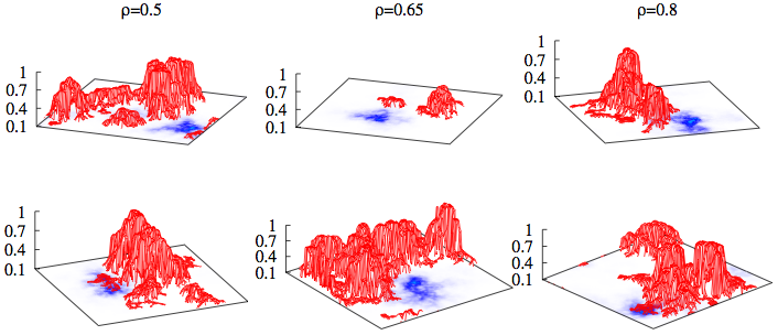
Figure 4: Red surfaces correspond to the absolute value of the magnetization of the spins in a $100\times 100$ system, while the contours (shadowed blue areas) mark the regions where the non convergence appears for the first time. For each of the three values of $\rho$, two different realizations of the disorder are shown. The xy-plane is set at magnetization $|m|=0.1$. In most cases the convergence problems appear in the low magnetization regions.

The above argument well explains the similarity between $T_{\text{CVM}}$ and $T_{\text{conv}}$ in the region $\rho<\rho^{cr}_{Kikuchi}$ where no ferromagnetic long range order is expected to take place. However, for $\rho>\rho^{cr}_{Kikuchi}$, the situation is more delicate: indeed there is ferromagnetic long range order below the critical line, and so the above argument can not hold as it is (there are no large regions with null local magnetizations, where the instability can easily arise). Moreover if we assume that a GBP instability can mainly grow in a region of low magnetizations, we would conclude that GBP must be much more stable for $\rho>\rho^{cr}_{Kikuchi}$. Indeed what we see in Fig. 3 is that the behavior of the filled squares drastically change around $\rho^{cr}_{Kikuchi}$, and $T_{\text{conv}}$ becomes much smaller in the ferromagnetic phase. This observation supports the idea that an instability of GBP can mainly arise and grow in a region of low local magnetizations: in a ferromagnetic phase these regions are rare and small, and thus GBP is able to converge down to very low temperatures.

IV.1 Average case with population dynamics

Recently in reference Domínguez et al. (2011) we have studied in detail the behavior of GBP on the 2D EA model (i.e. the present model with $\rho=0.5$). For this particular case we reported the two important temperatures: a critical temperature $T_{c}$ where the EA order parameter $q_{EA}$ predicted by the GBP becomes different from zero and a lower temperature $T_{\text{conv}}$ where GBP stops converging to a fixed point. We noticed that the critical temperature found by the replica CVM method was close to $T_{\text{conv}}$, while a critical temperature close to $T_{c}$ could also be obtained from an average case calculation based on a population dynamics method, similar to the one used in Mézard and Parisi (2001) for the Bethe approximation.

In the population dynamics method we have to evolve a population of 4-fields, corresponding to two small-$u$ messages and a triplet $(U,u_{1},u_{2})$ message arriving on the same pair of spins (see Fig. 5). Thanks to a local gauge symmetry, that is worth breaking in order to improve the algorithm convergence properties Domínguez et al. (2011), we can always set to zero one of the small-$u$ messages in triplet (hence the name 4-field). In the average case, the correlation between the Plaquette-to-Link and the Link-to-Spin fields is accounted in the 4-fields structure, but different 4-fields are considered uncorrelated around the plaquette. By randomly sampling the population and the couplings distribution new 4-fields are computed as schematically represented in Fig. 5. After many iterations the population stabilizes. The critical temperature is defined as the point where non-zero small $u$ messages appear in the population of 4-fields and turns out to be very close to the the value of $T_{c}$ computed in single instances. In ref. Domínguez et al. (2011) these facts were reported as an interesting coincidence that now we extend to other values of $\rho$.

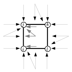
Figure 5: Population dynamics basic step. Four 4-fields $(u_{L\to i},U_{P\to ij},u_{P\to j},u_{L\to j})$ are taken at random from the population, and new 4-fields are computed inside the square with random couplings. The new 4-fields (one of which is shown in gray) are added back to the population.

In the right panel of Figure 3 the upper dotted line marks the critical temperatures obtained by the gauge fixed (GF) population dynamics method. The key observation is that this temperature is quite close to the single instance critical temperature $T_{c}$ of the GBP message passing algorithm. Moreover in Domínguez et al. (2011) we showed that the small discrepancy between the GF-SG critical temperature and the $T_{c}$ measured on single samples decreases by increasing the sample size. The closeness of these two temperatures suggests that the messages (4-fields) arriving on a plaquette in a 2D lattice are almost uncorrelated and thus lead to results similar to those obtained by a population dynamics, where messages are uncorrelated by construction. So the critical temperature $T_{c}$ for a given large sample can very well be estimated from the average case GF population dynamics. At the same time, it suggests that fixing the gauge and keeping the correlation among the 4 fields in a 4-field message is important to get the right critical temperature, but in the average case replica calculation we can not fix the gauge and the correlation among the 4 fields is disregarded, since the distributions $Q(U,u_{1},u_{2})$ and $q(u)$ are independent. This is a weakness of the replica calculation in describing the actual behavior of message passing algorithm on given samples.

In the Bethe approximation, a population dynamics of Link to Spin fields reproduces exactly the same critical temperature found by the replica method Mézard and Parisi (2001). We tried to implement a new population dynamics, where all messages in a plaquette are updated at the same time, given the messages entering the plaquette, but the critical temperatures found do not compare well with BP–$T_{c}$. We also got not better results by simulating in Bethe approximation a population of the 2-fields $(u_{1},u_{2})$ that enter the plaquette from one side.

These facts point in either of two directions. The first possibility is that the closeness of the GF population dynamics critical temperature (GF-SG in Fig. 5) to the critical temperature $T_{c}$ in single instances is completely casual. The second is that the population dynamics is actually related to the single instance behavior. In this latter case, the fact that in Bethe approximation the population dynamics is useless in identifying $T_{c}$ implies that not only the correlation kept in the 4-fields is crucial, but also the presence of the $U$-fields, somehow overruling the actual interactions in the plaquettes, is very important.

V Non-linear regime

Supported by the positive results of the previous sections, we look for the solution of the equations (II) in the non-linear regime, below $T_{\text{CVM}}$. Still, the complete deconvolution of the second equation is beyond our technical capabilities and we reduce again the problem to that of computing the different moments of the functions $q$ and $Q$. However, now we keep the effect of the small messages beyond the linear regime. We show results for $\rho=0.5$ such that $m$ and $M_{i}(U)$ are zero. But the extension to more general cases is straightforward.

We start parametrizing $Q(U,u_{1},u_{2})$ in the following way:

$$Q(U,u_{1},u_{2})=a_{0}(U)\phi(u_{1},u_{2})\;,$$ (24)

where

$$\phi(u_{1},u_{2})=(1-p_{U}-q_{U})\delta(u_{1})\delta(u_{2})+p_{U}\Big{[}\delta(u_{1}-\sqrt{a})\delta(u_{2}-\sqrt{a})+\delta(u_{1}+\sqrt{a})\delta(u_{2}+\sqrt{a})\Big{]}+\\ +q_{U}\Big{[}\delta(u_{1}-\sqrt{a})\delta(u_{2}+\sqrt{a})+\delta(u_{1}+\sqrt{a})\delta(u_{2}-\sqrt{a})\Big{]}\;.$$ (25)

Figure 6: Schematic representation of the parametrization for $Q(U,u_{1},u_{2})$

This parametrization is sketched in Figure 6. It is important to point out that the function $\phi$ is not necessarily positive, and that the parameters $p_{U}$ and $q_{U}$ depend on $U$, so are functions themselves. We proceed writing these parameters in terms of the moments of the distribution $Q$. This is easily done substituting (24) in (11)

$$a_{11}(U) = \int du_{1}du_{2}Q(U,u_{1},u_{2})u_{1}^{2}=a_{0}(U)[2a(p_{U}+q_{U})]\;,$$ (26)

$$a_{12}(U) = \int du_{1}du_{2}Q(U,u_{1},u_{2})u_{1}u_{2}=a_{0}(U)[2a(p_{U}-q_{U})]\;.$$ (27)

such that

$$p_{U} = \frac{a_{11}(U)+a_{12}(U)}{4\,a\,a_{0}(U)}\;,$$ (28)

$$q_{U} = \frac{a_{11}(U)-a_{12}(U)}{4\,a\,a_{0}(U)}\;.$$ (29)

Figure 7: Schematic representation of the parametrization for $q(u)$

Within this parametrization $a$ fixes the deviation from the paramagnetic solution of the distribution $Q$. But $a$ is defined by the distribution of the small messages $q(u)$. Therefore we keep the consistency in the equations, without loosing physical insight, parametrizing also the $q(u)$ in terms of $a$. The simplest parametrization is sketched in Figure 7. It reads:

$$q(u)=\frac{1}{2}\Big{[}\delta(u-\sqrt{a})+\delta(u-\sqrt{a})\Big{]} a>0$$ if

$$q(u)=2\delta(u)-\frac{1}{2}\Big{[}\delta(u-\sqrt{|a|})+\delta(u-\sqrt{|a|})\Big{]} a<0$$ if

Note that the case $a<0$ must be taken into consideration because, since $Q$ is not necessarily positive defined Rizzo et al. (2010), during the message passing procedure $a$ may become negative. Now, specializing the computations to the case of the triangular lattice, the integrals over $R(U,u_{1},u_{2})$ in (III) take the form

$$a_{11}(U)=\int du_{1}du_{2}R(U,u_{1},u_{2})u_{1}^{2}-aa_{0}(U)=\int dU^{a}dU^{b}a_{0}(U^{a})a_{0}(U^{b})\\ \int d\vec{u}^{a}d\vec{u}^{b}\phi(u^{a}_{1},u^{a}_{2})\phi(u^{b}_{1},u^{b}_{2})\prod_{i=1}^{4}q(u_{i})\hat{u}_{1}^{2}\delta(U-\hat{U}(\#))-aa_{0}(U)\;,$$ (30)

$$a_{12}(U)=\int du_{1}du_{2}R(U,u_{1},u_{2})u_{1}u_{2}=\int dU^{a}dU^{b}a_{0}(U^{a})a_{0}(U^{b})\\ \int d\vec{u}^{a}d\vec{u}^{b}\phi(u^{a}_{1},u^{a}_{2})\phi(u^{b}_{1},u^{b}_{2})\prod_{i=1}^{4}q(u_{i})\hat{u}_{1}\hat{u}_{2}\delta(U-\hat{U}(\#))\;,$$ (31)

and $a$ satisfies

$$a=\int dU^{a}dU^{b}a_{0}(U^{a})a_{0}(U^{b})\int d\vec{u}^{a}d\vec{u}^{b}\phi(u^{a}_{1},u^{a}_{2})\phi(u^{b}_{1},u^{b}_{2})\prod_{i=1}^{5}q(u_{i})\hat{u}^{2}(\#)\;,$$ (32)

where the integrals over $U$ are done using a standard population dynamics and the integrals over $\vec{u}$ can be computed exactly thanks to the previous ansatz [keep in mind that $\phi(u^{a}_{1},u^{a}_{2})$ is given by (25)]. The analysis for any other lattice is completely equivalent. Independently of the structure of the plaquettes, or the lattice dimensions the previous ansatz is always valid and the fixed point equations can be always reduced to expressions similar to (30)-(32). Only the computational effort may change. For example, while in equations (30) and (31) we integrate over two $U$ messages, $U^{a}$ and $U^{b}$, in the square lattice we will need a third message to integrate over. However, from the results obtained in the previous section we do not expect any gain in physical insight from studying the square lattice and we concentrate our efforts on the triangular lattice.

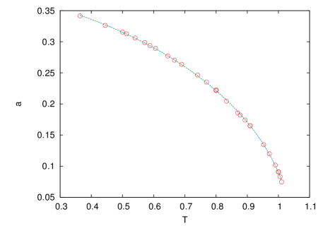
Figure 8: The $a$ parameter for the triangular lattice in the low temperature phase. The curve is a fit behaving as $(T_{\text{CVM}}-T)^{1/2}$ close to the critical point.

Our first result is presented in Figure 8 where we present the dependence of $a$ with $T$ below $T_{\text{CVM}}$. Note that the data is compatible with a behaviour of the form $a\propto(T_{\text{CVM}}-T)^{1/2}$, although analytical arguments would suggest a linear behavior in $(T_{\text{CVM}}-T)$, much as in the Bethe approximation case. It may be that the linear coefficient is actually very large but we did not further investigate this point because it would require a consistent increase of numerical precision in the critical region.

In presence of an external field, the symmetry which allow for the existence of polynomial algorithm to solve the 2D EA model Poulter and Blackman (2001); Thomas and Middleton (2009) breaks down. On the other hand the method based of the replica CVM equations can be perfectly used also in presence of an external field: the equations remain practically the same, with the only difference that the external field must be added to the local field $h$ in all the expressions above. We leave for the interested reader to prove this.

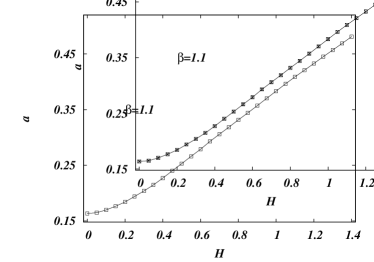
Figure 9: The $a$ parameter (left) and the energy $E$ (right) versus the external field $H$. The temperature is slightly below the Paramagnetic-Spin Glass phase transition ($\beta=1.1$).

We study the model in the presence of an external magnetic field, near, but below, the transition temperature and show (see Figure 9) that both $a$ and the energy $E$ go as $H^{2}$ close to the transition. Our results, although approximate, can be considered as a good starting point to study the role of the external field in finite dimensional lattices.

Figure 10: Distribution $a_{0}(U)$ of the messages $U$ at zero temperature, using the paramagnetic ansatz [left] and the non-linear ansatz of eq.(24) [right].

Finally we prove that this technique can be extended to zero temperature and provides non trivial informations also in that limit. In Figure 10 we show the structure of $a_{0}(U)$ considering a paramagnetic ansatz (left) where $\phi(u_{1},u_{2})=\delta(u_{1})\delta(u_{2})$ and $q(u)=\delta(u)$, and after reaching the fixed point of equations (30)-(32) (right). The paramagnetic solution has a structure very similar to the one found in the study of the EA model on a Bethe lattice Mézard and Parisi (2003). This is not surprising since within the paramagnetic ansatz the problem is equivalent to a Bethe approximation on the dual lattice (see our previous work Lage-Castellanos et al. (2011) for a larger discussion on this subject). On the other hand, the structure of $a_{0}(U)$ when non-linear effects are considered is richer. While the $U=0$ peak still dominates the distribution, and there is some reminiscence of other peaks, now the distribution spreads over non-integer values. This is probably one of the more remarkable mathematical consequences of the Kikuchi approximation. It is enough to consider the equation for $\hat{U}$ in the presence of small $u$’s, to understand that it is not possible to keep the self-consistency of the equations with distributions supported in the integers (even at $T=0$). This unavoidable fact make the computations at $T=0$ as heavier as the computations at finite temperature and further contributes to make the Kikuchi approximation harder to deal than the Bethe approximation.

Figure 11: Self-correlations $a_{11}(U)$ (left) and cross-correlations $a_{12}(U)$ (right) of small $u$ messages, using the non-linear ansatz in eq.(24)

To further explore the role of $\phi(u_{1},u_{2})$ we plot $a_{11}(U)$ (left) and $a_{12}(U)$ (right) in Figure 11. It is interesting to note that while $a_{11}(U)$ presents a structure with multiple peaks resembling the structure of $a_{0}(U)$, there is no clear evidence of such a structure in $a_{12}(U)$. This suggests that self-correlations of the small $u$ messages strongly depend on $a_{0}(U)$, much more than what the cross-correlations do (these show a smooth curve at every $U$).

VI Conclusions

We study typical properties of the 2D Edwards-Anderson model with the Replica Cluster Variational Method at the RS level. Using a linearized version of the self-consistency equations we have obtained the $\rho$ vs $T$ phase diagram on the square and triangular lattices. We show that this phase diagram resembles much better the theoretical predictions, than the one obtained using the Bethe approximation: the SG critical temperature is lower, the tricritical point is closer to the exact value and the SG-Ferro phase boundary looks similar to theoretical expectations. Moreover, we present numerical evidences supporting the idea that the temperature below which the average case computation predicts the existence of a spin-glass phase ($T_{\text{CVM}}$) is also the temperature at which GBP algorithms stop converging. We apply to the triangular lattice a method to solve the RS equations in the non-linear regime, i.e., at very low temperatures. The method does work and we show results at $T=0$ and in the presence of an external magnetic field. All these results suggest that the replica CVM can be used to study finite-dimensional spin glasses, and hopefully in higher dimensions ($D>2$) the approximation should provide an even better description of the low temperature phase.

Appendix: Triangular lattice

We report here the expressions for the first and second moments of $Q(U,u_{1},u_{2})$ in the case of the triangular lattice.

$$M_{1}(U)=\langle\int dU^{a}dU^{b}\delta\big{(}U-\mathrm{arctanh}[\tanh(\beta(J^{a}+U^{a}))\tanh(\beta(J^{b}+U^{b}))]/\beta\big{)}\\ \Bigg{[}\frac{M_{1}(U^{a})a_{0}(U^{b})+a_{0}(U^{a})M_{1}(U^{b})}{2}+2m\tanh(\beta J_{+})+\tanh(\beta J_{+})\frac{M_{1}(U^{a})+M_{1}(U^{b})}{2}\Bigg{]}\rangle_{J}\;,$$ (33)

$$a_{11}(U)=\langle\int dU^{a}dU^{b}\delta\big{(}U-\mathrm{arctanh}[\tanh(\beta(J^{a}+U^{a}))\tanh(\beta(J^{b}+U^{b}))]/\beta\big{)}\\ \Bigg{[}\frac{a_{11}(U^{a})a_{0}(U^{b})+a_{0}(U^{a})a_{11}(U^{b})}{2}+2m\tanh(\beta J_{+})[M_{1}(U^{a})+M_{1}(U^{b})]+\\ +2m\tanh(\beta J_{-})[M_{1}(U^{a})-M_{1}(U^{b})]+\tanh(\beta J_{+})M_{1}(U^{a})M_{1}(U^{b})+\\ \frac{1}{2}\tanh(\beta J_{+})[a_{12}(U^{a})+a_{12}(U^{b})]+\frac{1}{2}\tanh(\beta J_{-})[a_{12}(U^{a})-a_{12}(U^{b})]+\\ (a+3m^{2})[\tanh^{2}(\beta J_{+})+\tanh^{2}(\beta J_{-})]+2m[\tanh^{2}(\beta J_{+})+\tanh^{2}(\beta J_{-})][M_{1}(U^{a})+M_{1}(U^{b})]+\\ \frac{1}{4}[\tanh^{2}(\beta J_{+})+\tanh^{2}(\beta J_{-})][a_{11}(U^{a})+a_{11}(U^{b})+2M_{1}(U^{a})M_{1}(U^{b})]\Bigg{]}\rangle_{J}\;,$$ (34)

$$a_{12}(U)=\langle\int dU^{a}dU^{b}\delta\big{(}U-\mathrm{arctanh}[\tanh(\beta(J^{a}+U^{a}))\tanh(\beta(J^{b}+U^{b}))]/\beta\big{)}\\ \Bigg{[}M_{1}(U^{a})M_{1}(U^{b})+2m[\tanh(\beta J_{+})(M_{1}(U^{b})+M_{1}(U^{a}))+\tanh(\beta J_{-})(M_{1}(U^{b})-M_{1}(U^{a}))]+\\ \frac{1}{2}\tanh(\beta J_{+})[2M_{1}(U^{a})M_{1}(U^{b})+a_{12}(U^{a})+a_{12}(U^{b})]+\tanh(\beta J_{-})\frac{a_{12}(U^{b})-a_{12}(U^{a})}{2}+\\ (a+3m^{2})(\tanh^{2}(\beta J_{+})-\tanh^{2}(\beta J_{-}))+2m[\tanh^{2}(\beta J_{+})-\tanh^{2}(\beta J_{-})][M_{1}(U^{a})+M_{1}(U^{b})]+\\ \frac{1}{4}[\tanh^{2}(\beta J_{+})-\tanh^{2}(\beta J_{-})][a_{11}(U^{a})+a_{11}(U^{b})+2M_{1}(U^{a})M_{1}(U^{b})]\Bigg{]}\rangle_{J}\;,$$ (35)

where $J_{+}=(J^{a}+U^{a})+(J^{b}+U^{b})$, $J_{-}=(J^{a}+U^{a})-(J^{b}+U^{b})$.

References

- Edwards and Anderson (1975) S. F. Edwards and P. W. Anderson, J. Phys. F, 5, 965 (1975).
- Parisi (1979) G. Parisi, Physics Letters A, 73, 203 (1979).
- Parisi (1980) G. Parisi, J. Phys. A, 13, L115 (1980).
- Kirkpatrick and Sherrington (1978) S. Kirkpatrick and D. Sherrington, Phys. Rev. B, 17, 4384 (1978).
- Parisi et al. (1987) G. Parisi, M. Mézard, and M. Virasoro, Spin Glass Theory and Beyond (World Scientific, Singapore, 1987).
- Marinari et al. (2000) E. Marinari, G. Parisi, F. Ricci-Tersenghi, J. J. Ruiz-Lorenzo, and F. Zuliani, J. Stat. Phys., 98, 973 (2000).
- Mézard and Parisi (2001) M. Mézard and G. Parisi, Eur. Phys. J. B, 20, 217 (2001).
- Mézard and Parisi (2003) M. Mézard and G. Parisi, J. Stat. Phys., 111, 1 (2003).
- Viana and Bray (1985) L. Viana and A. J. Bray, J. Phys. C, 18, 3037 (1985).
- Mezard et al. (2002) M. Mezard, G. Parisi, and R. Zecchina, Science, 297, 812 (2002).
- Mézard and Zecchina (2002) M. Mézard and R. Zecchina, Phys. Rev. E, 66, 056126 (2002).
- Mulet et al. (2002) R. Mulet, A. Pagnani, M. Weigt, and R. Zecchina, Phys. Rev. Lett., 89, 268701 (2002).
- Braunstein et al. (2003) A. Braunstein, R. Mulet, A. Pagnani, M. Weigt, and R. Zecchina, Phys. Rev. E, 68, 036702 (2003).
- Zhou (2003) H. Zhou, Eur. Phys. J. B, 32, 265 (2003).
- Pearl (1988) J. Pearl, Probabilistic Reasoning in Intelligent Systems: Networks of Plausible Inference (Morgan Kaufmann, San Fransico, CA, 1988).
- Kabashima and Saad (1998) Y. Kabashima and D. Saad, Europhys. Lett., 44, 668 (1998).
- Montanari and Rizzo (2005) A. Montanari and T. Rizzo, J. Stat. Mech., P10011 (2005).
- Chertkov and Chernyak (2006) M. Chertkov and V. Y. Chernyak, Phys. Rev. E, 73, 065102 (2006a).
- Chertkov and Chernyak (2006) M. Chertkov and V. Y. Chernyak, J. Stat. Mech., P06009 (2006b).
- Mooij and Kappen (2007) J. M. Mooij and H. J. Kappen, J. Mach. Learn. Res., 8, 1113 (2007).
- Gomez et al. (2010) V. Gomez, H. J. Kappen, and M. Chertkov, J. Mach. Learn. Res., 11, 1273 (2010).
- Xiao and Zhou (2011) J.-Q. Xiao and H. Zhou, J. Phys. A, 32, 425001 (2011).
- Yedidia et al. (2005) J. Yedidia, W. T. Freeman, and Y. Weiss, IT-IEEE, 51, 2282 (2005).
- Kikuchi (1951) R. Kikuchi, Phys. Rev., 81, 988 (1951).
- Rizzo et al. (2010) T. Rizzo, A. Lage-Castellanos, R. Mulet, and F. Ricci-Tersenghi, J. Stat. Phys., 139, 375 (2010).
- Domínguez et al. (2011) E. Domínguez, A. Lage, R. Mulet, F. Ricci-Tersenghi, and T. Rizzo, J. Stat. Mech., P12007 (2011).
- Pelizzola (2005) A. Pelizzola, J. Phys. A, 38, R309 (2005).
- Monasson (1998) R. Monasson, J. Phys. A, 31, 513 (1998).
- Lage-Castellanos et al. (2011) A. Lage-Castellanos, R. Mulet, F. Ricci-Tersenghi, and T. Rizzo, Phys. Rev. E, 84, 046706 (2011).
- Mézard and Montanari (2009) M. Mézard and A. Montanari, Information, Physics and Computation (Oxford University Press, Cambridge, 2009).
- Takeda et al. (2005) K. Takeda, T. Sasamoto, and H. Nishimori, J. Phys. A, 38, 3751 (2005).
- Nishimori and Ohzeki (2006) H. Nishimori and M. Ohzeki, J. Phys. Soc. Japan, 75 (2006).
- Poulter and Blackman (2001) J. Poulter and J. Blackman, J. Phys. A, 34, 7527 (2001).
- Zhou et al. (2012) H. Zhou, C. Wang, J.-Q. Xiao, and Z. Bi, J. Stat. Mech., L12001 (2012).
- Griffiths (1969) R. B. Griffiths, Phys. Rev. Lett., 23, 17 (1969).
- Vojta (2006) T. Vojta, Journal of Physics A: Mathematical and General, 39, R143 (2006).
- Thomas and Middleton (2009) C. K. Thomas and A. A. Middleton, Phys. Rev. E, 80, 046708 (2009).