Chemo-mechanical instabilities in polarizable active layers

Abstract

We formulate and explore a generic continuum model of a polarizable active layer with neo-Hookean elasticity and chemo-mechanical interactions. Homogeneous solutions of the model equations exhibit a stationary long-wave instability when the medium is activated by expansion, and an oscillatory short-wave instability in the case of compressive activation. Both regimes are investigated analytically and numerically. The long-wave instability initiates a coarsening process, which provides a possible mechanism for the establishment of permanent polarization in spherical geometry.

Active media are capable to modify their mechanical properties under the influence of chemical signaling; in their turn, chemical transformations may be affected by local stress, strain and polarization. This creates a feedback loop that, on the one hand, makes rheology of the medium flexible and responsive to the environment and, on the other hand, may cause various instabilities, leading to spatial inhomogeneities, oscillations, and spontaneous motion. The primary example of an active biological medium is cytoskeleton, which is the principal structural element of eukaryotic cells responsible for their integrity, reshaping, proliferation, and motion Howard (2001); Lieleg et al. (2010).

Experimental studies of living tissues give many examples of instabilities involving chemo-mechanical interactions, such as spontaneous oscillatory contraction of muscle fibers Fujita and Ishiwata (1998), traveling waves Gerisch et al. (2004), and intermittent localized oscillations in vivo Martin (2010) that occur, in particular, during such tissue reshaping processes as dorsal closure Solon et al. (2009); Gorfinkiel et al. (2011) and elongation of the Drosophila egg shell He et al. (2010). Inhomogeneities and patterns of non-genetic origin are inconspicuous in vivo but are prominent in model systems, seen as clusters, swirls and interconnected bands in motility assays Schaller et al. (2010), localized motor activity spots in reconstituted actin-myosin mixtures Silva et al. (2011), and velocity spurts in spreading tissues Petitjean et al. (2010). Mechanical impact on chemical oscillations (though without feedback reaction) has been also detected in inorganic gels Kuksenok et al. (2007).

Mechanisms of chemo-mechanical interactions in living cells and tissues are variegated and largely unknown but underlying general characteristics can be understood by taking as a basis well-established principles of continuous mechanics that account for the symmetries of the medium, and imposing a simple chemical feedback. The continuum approximation is particularly suitable for analytical studies of instability thresholds. Symmetry-breaking and oscillatory instabilities due to chemo-mechanical coupling have been detected in this way in the context of calcium transfer dynamics Murray and Oster (1984); Oster and Odell (1984), and much later with myosin motors acting as chemical variables Banerjee and Marchetti (2011). Further studies included nematic polarization in the continuum theory Kruse et al. (2005); Jülicher et al. (2007) based on de Gennes’ description of nematic liquid crystals de Gennes and Prost (1993) and adding a term proportional to chemical potential to account for the biological activity. The resulting equations of polar gels are quite formidable but their simplified versions have enabled elegant description of structures and defects in nematic gels Jülicher et al. (2007), spontaneous flow Doubrovinski and Kruse (2011); Fürthauer et al. (2012), and other phenomena in polar active media.

In this Letter, we explore an alternative case of a medium with vector polarization. The source of polarization of cytoskeleton is directionality of actin filaments characterized by a unique direction of treadmilling and motion of myosin motors. In acto-myosin stress fibers, nematic order prevails due to periodic polarity alternation as, for example, in sarcomeric structures. On the other hand, stress fibers in motile cells have a graded polarity pattern Deguchi and Sato (2009) implying vector polarization. This kind of polarization is essential for generation of active forces that play a primary role in tissue spreading Nikolic et al. (2006); Poujade et al. (2007); Salm and Pismen (2012). Another distinctive feature of our approach is allowing for spontaneous emergence of polarization, alongside with mechanical deformation and chemical activity, whereas in earlier studies of polar active media, with few exceptions Salbreux et al. (2009), only the direction, rather than the absolute value of the nematic order parameter was evolving dynamically. After formulating dynamic equations applicable to a thin flat polarizable deformable layer on a solid substrate, we will determine analytically the various instabilities thresholds, and further explore numerically the evolution of emerging patterns using the neo-Hookean formulation applicable to strongly deformable soft matter Ogden (2001).

Dynamics of thin layers dominated by friction is Aristotelian (overdamped), with velocity rather than acceleration proportional to the force. Close to equilibrium, the force driving the evolution of any dynamic variable $\Psi$ can be derived from an appropriate energy functional ${\cal F}\{\Psi\}$, leading to a dynamic equation in the variational form $\Gamma\,\mathrm{D}_{t}\Psi=-\delta{\cal F}/\delta\Psi$, where D${}_{t}=\partial_{t}+\mathrm{v}\cdot\nabla$ is the substantial derivative, v is the local velocity, and $\Gamma$ is an appropriate friction coefficient. We will write in this form basic dynamic equations for the deformation and polarization fields, and further add non-equilibrium terms accounting for the active character of the medium.

The medium is assumed to be incompressible but it can stretch in the horizontal plane $\mathbf{x}$, while modifying the layer thickness $h$. Since the vertical deformation is small compared to the deformations in the horizontal plane and the latter, in turn, are uniform in the vertical direction, the elastic energy is expressed through the two-dimensional (2D) strain tensor. Let $\mathbf{x},\,\mathbf{X}(\mathbf{x})$ be the dimensionless position vectors, respectively, in the reference (stress-free) and deformed states. The components of the strain tensor are $\omega_{ij}=\partial_{i}X_{k}\partial_{j}X_{k}-\delta_{ij}$, where $\delta_{ij}$ is the Kronecker delta; summation over repeated indices is presumed here and below. The elastic energy is

$$\mathcal{F}_{\mathrm{el}}=\int\mathcal{L}_{\mathrm{el}}{\rm d}^{2}\mathbf{x},\quad{\cal L}_{\mathrm{el}}=\mu h{\cal L}_{0},\quad{\cal L}_{0}=\frac{1}{4}\omega_{ij}\omega_{ij}.$$ (1)

where $\mu$ is the shear modulus.

Unlike the standard 2D formulation, the variation of $h$ should be taken into account when the dynamic equations are derived. In view of the incompressibility, $h=h_{0}J^{-1}$, where $h_{0}$ is the unperturbed thickness and $J$ is the determinant of the 2D matrix with the components $\partial_{j}X_{i}$. We write the dynamic equations in the dimensionless form

$$\eta\,\mathrm{D}_{t}X_{i}=\frac{1}{2}\partial_{j}\left(\frac{\omega_{jk}}{J}\partial_{k}X_{i}-\frac{{\cal L}_{0}}{J^{2}}\epsilon_{ik}\epsilon_{jl}\partial_{l}X_{k}\right)+\frac{f_{i}}{2J},$$ (2)

where $\mathbf{F}=(\mu/a_{x})\,\mathbf{f}$ is an active force per unit volume (to be specified below), $\eta=\Gamma_{\mathrm{el}}a_{x}^{2}/(2\mu h_{0}a_{t})$, $a_{x},\,a_{t}$ are the length and time scales, and $\epsilon_{ik}$ is the 2D antisymmetric matrix.

Planar polarization is characterized by the 2D vector order parameter $\mathbf{p}(\mathbf{X},t)$. The polarization energy is expressed as an integral over the deformed domain: $\mathcal{F}_{\mathrm{p}}=\int\mathcal{L}_{\mathrm{p}}{\rm d}^{2}\mathbf{X}$, where the Lagrangian ${\cal L}_{p}$ should be expressed through rotationally invariant combinations of $\mathbf{p}$ and the 2D gradient operator $\nabla$ with respect to the coordinates $X_{i}$. Retaining terms with the added orders in $\mathbf{p}$ and $\nabla$ not exceeding four, we write

$${\cal L}_{\mathbf{p}} = \frac{\kappa h}{2a_{x}^{2}}\left[\alpha^{2}|\mathbf{p}|^{2}\left(1+\frac{\kappa_{0}}{2}|\mathbf{p}|^{2}\right)+2\kappa_{1}\nabla_{i}p_{i}\right.$$ (3)

$$+ \left.(\nabla_{i}p_{i})^{2}+\kappa_{2}(\epsilon_{ik}\nabla_{i}p_{k})^{2}+\kappa_{3}|\mathbf{p}|^{2}\nabla_{i}p_{i}\right].$$

The second term is irrelevant, unless the coefficient $\kappa_{1}$ couples the order parameter with another field. In an active medium, this might be the concentration $c$ of some chemical species. We choose $\kappa_{0}^{-1/2}$ as the polarization scale and set $\kappa_{1}=-\kappa_{0}^{-1/2}c$, where $c(\mathbf{X},t)$ is interpreted as a scaled deviation from a reference concentration $c_{0}$. Setting also $\kappa_{3}=0$, we write the dynamic equation generated by the Lagrangian (3) in the dimensionless form

$$\gamma\,\mathrm{D}_{t}p_{i} = \nabla_{i}(J^{-1}\nabla_{j}p_{j})+\kappa_{2}\nabla_{j}\left[J^{-1}\left(\nabla_{j}p_{i}-\nabla_{i}p_{j}\right)\right]$$ (4)

$$- \nabla_{i}(J^{-1}c)-\alpha^{2}J^{-1}\left(1+|\mathbf{p}|^{2}\right)p_{i},$$

where $\gamma=\Gamma_{\mathbf{p}}a_{x}^{2}/(\kappa h_{0}a_{t})$. Generally, one has to include the variation of the polarization energy into the deformation equations; indeed, a polarized medium may deform to releave polarization gradients. We will avoid, however, this complication, assuming $\kappa\ll\mu$. The coupling between polarization and deformation will be established instead by the active force in Eq. (2) directed along the polarization direction, $f_{i}=2qp_{i}$.

The feedback loop is closed by making concentration of the active species strain-dependent. We write the equation of the concentration field taking into account that, due to incompressibility, the concentration is not affected by deformation; the diffusional flux is, however, proportional to the local thickness. Allowing for the production rate proportional to the local strain and linear decay with the constant identified with the inverse time scale $1/a_{t}$, we write the concentration equation in the dimensionless form

$$\mathrm{D}_{t}c=J\nabla_{i}(J^{-1}\nabla_{i}c)-c+\beta(J-1).$$ (5)

where we have chosen as the length scale the diffusion length $a_{x}=\sqrt{Da_{t}}$, $D$ being the diffusivity.

The above equation system becomes extremely convoluted if applied in a fixed coordinate frame where, besides computing the substantial derivative that includes the velocity $\mathbf{v}=\partial_{t}\mathbf{X}$, one would need to transform the $\nabla$ operator in Eqs. (4), (5) to account for deformations. These complications do not affect, however, linear stability analysis, and will be avoided at large deformations by implementing a Lagrangean numerical procedure.

Figure 1: Stability diagram in the parametric plane $\alpha,\>\beta q$. The oscillatory instability limits are shown for $\gamma=5/4$ and $\eta=1/3$ (solid line), $\eta=5/3$ (dashes), and $\eta=10/3$ (dots). Inset: the critical wavelength $k$ at the oscillatory bifurcation lines parameterized by $\alpha$.

We explore now stability of the homogeneous solution $\mathbf{p}=0$, $c=0$, $\mathbf{X}=\mathbf{x}$ to infinitesimal perturbations. The linearized system determining the bifurcation threshold can be expressed through the 2D strain $\psi=J-1=\nabla_{i}(X_{i}-x_{i})$ and splay $\phi=\nabla_{i}p_{i}$ by taking the divergence of linearized Eqs. (2), (4):

$$\eta\,\partial_{t}\psi = \nabla^{2}\psi+q\phi,$$ (6)

$$\gamma\,\partial_{t}\phi = \nabla^{2}\phi-\alpha^{2}\phi-\nabla^{2}c,$$ (7)

$$\partial_{t}c = \nabla^{2}c-c+\beta\psi.$$ (8)

A nontrivial solution of Eqs. (6) – (8) is sought for as a waveform $\exp(\lambda t+{\rm i\,}\mathbf{k}\cdot\mathbf{x})$ with a wave vector $\mathbf{k}$. The eigenvalues $\lambda$ determining stability of the uniform state $c=\psi=\phi=0$ are computed by setting to zero the determinant of the Fourier transformed linearized system. The bifurcation thresholds are computed in a standard way by requiring $\sup_{|\mathbf{k}|}(\Re\lambda)=0$.

In the case of extentional activation ($\beta>0$), one can show that the branch of real eigenvalues first reaches zero in the long-wave mode $\mathbf{k}=0$ at $\beta q=\alpha^{2}$. In the case of compressive activation ($\beta<0$), a wave instability at finite $|\mathbf{k}|$ and $\Im\lambda\neq 0$ is observed. The analytic formulas for the critical wavenumber $k_{\mathrm{c}}$ and the critical value $\beta_{\mathrm{c}}$ are too cumbersome to be of practical use and will not be listed here. The minimal gap width between the two instability limits equals to $\gamma+\eta$. The bifurcation diagram in the parametric plane $\alpha,\,\beta q$ is shown in Fig. 1.

We explore dynamics beyond the bifurcation thresholds for both types of activation by direct numerical simulation, starting from randomly perturbed homogeneous initial conditions. We discretize Eqs. (2), (4), and (5) using a flexible grid with nodes following the physical displacement of the medium. In the spirit of mesh-free computations Onate et al. (1996), the spatial derivatives are calculated based on local approximation of the fields by low-order polynomials. The resulting set of ordinary differential equations is then solved using an embedded adaptive Runge-Kutta-Fehlberg scheme of the order 4 and 5 Press (1999). The parameters are set to $q=\sqrt{5}/100,\alpha=\sqrt{5},\kappa_{2}=1,\eta=5/3,\>\gamma=5/4$.

In the oscillatory regime, we observe a wave pattern with the active force (directed from high to low $c$ regions) following the rotating concentration gradient between the domains oscillating in antiphase, as seen in Fig. 2. The directions of the elastic and active force are, however, disaligned due to delay, so that the angle between the two is widely distributed with a shallow maximum about $\pi/2$ (Fig. 3).

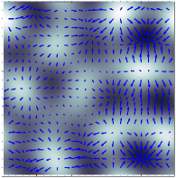
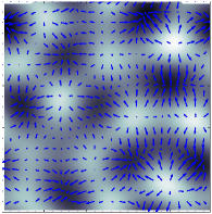
Figure 2: Snapshots from a simulation in the oscillatory unstable parametric region ($\beta q=-210$, $(\beta q)_{c}\approx-196$). The time difference between the two images equals half the oscillation period. The simulation domain is a double-periodic $10\sqrt{5}\times 10\sqrt{5}$ square. Lighter shades correspond to higher concentration levels; scaled arrows indicate the polarization $\mathbf{p}$.

Figure 3: Histogram of the angle $\varphi$ between the directions of the elastic and active force.

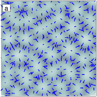
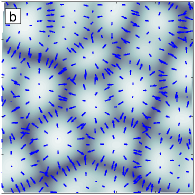
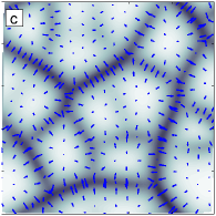
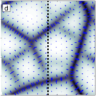
Figure 4: Domain coarsening: snapshots at $t=4\times 10^{3}$ (a), $2\times 10^{4}$ (b), $3\times 10^{4}$ (c), $5\times 10^{4}$ (d), simulation on the double-periodic $100\sqrt{5}\times 100\sqrt{5}$ square domain for $\beta q=6$, $(\beta q)_{c}=5$.

Figure 5: Time evolution of the wavelength of the dominant Fourier mode during coarsening (the average of $30$ simulations on the double-periodic $100\sqrt{5}\times 100\sqrt{5}$ square domain for $\beta q=6$).

In the case of extensional activation, the behavior is qualitatively different. Initially, a short-wave pattern corresponding to a fastest-growing mode emerges from the initial noise. Then, a slow coarsening process ensues, during which larger domains grow while smaller ones either merge or vanish, so that the dominant wavelength grows, as seen in Fig. 4. The wavelength corresponding to the maximum of the Fourier spectrum is plotted against time in Fig. 5. Due to the finite size of the simulation domain, the plot for each individual run has a number of discontinuous steps but it approaches a monotonically growing curve when averaged over $30$ runs.

Unlike the oscillatory case, the active and elastic forces are almost perfectly anti-aligned: the mutual angle deviates from $\pi$ by less than $3.5^{\circ}$ with $98\%$ probability. As the active force is directed against the concentration gradient, the low-$c$ regions are squeezed into narrow stripes separating high-$c$ domains. In turn, the chemical production is inhibited within these stripes due to strong compression, as the deformation acts as the source of $c$ in Eq. (5). The resulting correlation between $J$ and $c$ is seen in Fig. 6 that shows the cross-section profiles at a late stage of coarsening.

Figure 6: Cross section through the dashed line in Fig. 4 (d). The polarization component along the line $\mathbf{p}\cdot\mathbf{e}_{y}$ and deformation $J-1$ are scaled to show all three fields in the same plot.

Figure 7: Time evolution of the concentration $c$ at different polar angles $\theta$ on a sphere of radius $10\sqrt{5}$.

The coarsening process provides a natural mechanism for polarity establishment in cortical tissues, as is observed, for example, in the C. elegans embryo Cowan and Hyman (2007). When Eqs. (2), (4), and (5) are solved on a spherical surface, the coarsening consolidates two domains, whereafter the smaller one is compressed into a low-$c$ spot. This is illustrated in Fig. 7, where the evolution of $c$ is plotted for five different polar angles $\theta$, where $\theta=0$ is defined by the location of the high-concentration pole. As the polarization is aligned with the concentration gradient, the active force is directed from one pole to the other. The established polarity axis is permanent, unlike Ref. Goehring et al. (2011) where advection serves as a mere trigger requiring additional means for preserving the polarization.