Mutation Symmetries in BPS Quiver Theories:
      Building the BPS Spectra

Abstract:

We study the basic features of BPS quiver mutations in 4D $\mathcal{N}=2$ supersymmetric quantum field theory with $G=ADE$ gauge symmetries. We show, for these gauge symmetries, that there is an isotropy group $\mathcal{G}_{Mut}^{G}$ associated to a set of quiver mutations capturing information about the BPS spectra. In the strong coupling limit, it is shown that BPS chambers correspond to finite and closed groupoid orbits with an isotropy symmetry group $\mathcal{G}_{strong}^{G}$ isomorphic to the discrete dihedral groups $Dih_{2h_{G}}$ contained in Coxeter$\left(G\right)$ with $h_{G}$ the Coxeter number of G. These isotropy symmetries allow to determine the BPS spectrum of the strong coupling chamber; and give another way to count the total number of BPS and anti-BPS states of $\mathcal{N}=2$ gauge theories. We also build the matrix realization of these mutation groups $\mathcal{G}_{strong}^{G}$ from which we read directly the electric-magnetic charges of the BPS and anti-BPS states of $\mathcal{N}=2$ QFT₄ as well as their matrix intersections. We study as well the quiver mutation symmetries in the weak coupling limit and give their links with infinite Coxeter groups. We show amongst others that $\mathcal{G}_{weak}^{su_{2}}$ is contained in ${GL}\left({2,}\mathbb{Z}\right)$; and isomorphic to the infinite Coxeter ${I_{2}^{\infty}}$. Other issues such as building $\mathcal{G}_{weak}^{so_{4}}$ and $\mathcal{G}_{weak}^{su_{3}}$ are also studied.

1 Introduction

Recently a BPS quiver theory has been proposed in [1, 2] to build the full set of BPS spectra in 4D $\mathcal{N}=2$ supersymmetric quantum field theory (QFT₄) with rank $r$ gauge invariance $G_{r}$ given by the standard simply laced ADE symmetries. These massive and charged protected states of the Hilbert space of the $\mathcal{N}=2$ QFT₄, which are undetermined by the low energy theory alone; are remarkably described in the approach of [1, 2] relying on quantum mechanical dualities [3]. These dualities are encoded by quiver mutations relating distinct quivers living at different regions of the parameter space of the BPS theory. The originality of the quiver method is that it gives a new way to deal with general BPS states across the Coulomb branch $\mathcal{U}$; and proposes an explicit algorithm to deduce them. A key ingredient in the theory of [1, 2] is quiver mutations essentially based on the two following things:

(1) start from the ”primitive” BPS quiver, referred here to as $\mathfrak{Q}_{0}^{G}$, living at a point $u$ of the Coulomb branch, and made of the r elementary monopoles $\left(\mathfrak{M}_{1},...,\mathfrak{M}_{r}\right)$ and the $r$ elementary dyons $\left(\mathfrak{D}_{1},...,\mathfrak{D}_{r}\right)$ of the effective low-energy solutions of $\mathcal{N}=2$ supersymmetric gauge theory [4, 5]; see also  [6]-[22]. The $\mathfrak{M}_{i}$’s and $\mathfrak{D}_{i}$’s are thought of as the elementary building block of the BPS spectrum; and form a positive integral basis of the entire BPS spectrum. These elementary particle hypermultiplets have complex central charges Z respectively denoted here as $X_{i}$ and $Y_{i}$ with $\mathop{\mathrm{I}m}X_{i}>0,$ $\mathop{\mathrm{I}m}Y_{i}>0$; their absolute values $\left|X_{i}\right|$ and $\left|Y_{i}\right|$ give the masses of the BPS particles and their arguments $\arg X_{i}$, $\arg Y_{i}$ for distinguishing BPS chambers.
The $\mathfrak{M}_{i}$ and $\mathfrak{D}_{i}$ particle states live in the upper half plane $\mathcal{H}$ ($\mathop{\mathrm{I}m}Z>0$ of the complex $Z$ plane); and have electric-magnetic (EM) charges respectively given by the $2r$ components vectors $b_{i}=\left(0,\alpha_{i}\right),$ $c_{i}=\left(\alpha_{i},-\alpha_{i}\right)$ with intersections $b_{i}\circ c_{j}$ remarkably encoded by the Cartan matrix $K_{ij}=\alpha_{i}.\alpha_{j}$ of the Lie algebra of the ADE gauge symmetries.

(2) perform mutation transformations acting on the EM charges $b_{i}$ and $c_{i}$ mapping therefore the primitive $\mathfrak{Q}_{0}^{G}$ into mutated quivers $\mathfrak{Q}_{n}^{G}$, $n\geq 0$ describing the same physics as $\mathfrak{Q}_{0}^{G}$. From the obtained $\mathfrak{Q}_{n}^{G}$s we can learn the EM charges of the BPS states of the $\mathcal{N}=2$ supersymmetric QFT₄. In [1, 2], the quiver mutations have been realized as rotations $\mathcal{H}$ $\rightarrow$ $e^{-i\theta}\mathcal{H}$ in the half plane of the complex central charges; and have been interpreted  in terms of quantum mechanical dualities relating the BPS spectra of the quivers $\left\{\mathfrak{Q}_{n}^{G}\right\}$. This family of quivers lead to a chamber of BPS states with EM charges given by positive integer combinations of the charges of the elementary monopoles $b_{i}$ and dyons $c_{i}$.

In this paper, we contribute to this matter by studying the algebraic structure of the quiver mutations which we use to get the BPS spectra of the $\mathcal{N}=2$ QFT₄; and to interpret results obtained in [1, 2]. This algebraic approach may be also viewed as a way to deal with the complexity of the BPS content of the infinite weak coupling chambers of these supersymmetric QFT₄s. 
More precisely, if thinking about generic BPS quivers $\mathfrak{Q}_{n}^{G}$, $n\in\mathbb{N}$, of the pure ADE gauge theories as given by the pair

$$\mathbf{v}^{\left(n\right)}=\left(b^{\left(n\right)},c^{\left(n\right)}\right)$$ ,

(1)

with the $b_{i}^{\left(n\right)},$ $c_{i}^{\left(n\right)}$ entries of $\mathbf{v}^{\left(n\right)}$ describing the nodes of $\mathfrak{Q}_{n}^{G}$ and $\mathcal{A}^{\left(n\right)}$ their intersection matrix, the successive quiver mutations $\mathfrak{Q}_{0}^{G}$ $\rightarrow$ $\mathfrak{Q}_{1}^{G}$ $\rightarrow$ … $\rightarrow\mathfrak{Q}_{n}^{G}$, with positive integer n, can be thought of as particular morphisms $\mathcal{M}_{n}$ that can be then realized in terms of invertible matrices $\mathcal{M}_{n}$ belonging to a set $\mathcal{G}_{Mut}^{G}$ $\subset GL\left(4r^{2},\mathbb{Z}\right)$ and acting on the known elementary BPS quiver $\left\{\mathbf{v}^{\left(0\right)},\mathcal{A}^{\left(0\right)}\right\}$ as follows

$$\mathbf{v}^{\left(n\right)}=\mathcal{M}_{n}\mathbf{v}^{\left(0\right)}$$ ,

Clearly, the big $GL\left(4r^{2},\mathbb{Z}\right)$ is not a symmetry of the BPS quiver theory; only a particular subset $\mathcal{G}_{Mut}^{G}$ of it, to be explicitly built later, which is a symmetry. In this way of doing the data about quiver mutations; in particular the ones concerning the strong coupling BPS chamber considered in sections 3, 4, 5 and appendix II, are captured by the primitive $\mathfrak{Q}_{0}^{G}$ and the set $\left\{\emph{M}_{n};\text{ }n\in\mathbb{N}\right\}$ whose determination and their algebraic properties are therefore of major interest.

Now, if denoting by $L_{1}$ the mutation transformation that maps the elementary BPS quiver $\mathfrak{Q}_{0}^{G}$ into the mutated quiver $\mathfrak{Q}_{1}^{G}$, and by $L_{2}$ the mutation transformation mapping $\mathfrak{Q}_{1}^{G}$ into the mutated quiver $\mathfrak{Q}_{2}^{G}$; and in general by $L_{n}$ the mutation transformation that maps $\mathfrak{Q}_{n-1}^{G}$ into the mutated $\mathfrak{Q}_{n}^{G}$, the structure of the BPS spectra in the chamber based on $\mathfrak{Q}_{0}^{G}$, generated by successive $L_{n}$ actions, should be encoded in the following typical set

$$\mathcal{G}_{Mut}^{G}=\left\{\mathcal{M}_{m,0}:\mathfrak{Q}_{0}^{G}\rightarrow\mathfrak{Q}_{m}^{G};\text{ \ \ }m\in\mathbb{N}\right\}$$ (2)

with $\mathcal{M}_{m,0}\equiv\mathcal{M}_{m}$ realized by the morphisms product

$$\mathcal{M}_{m}=L_{m}L_{m-1}....L_{2}L_{1}$$ (3)

In the above relation, the matrix generators $L_{n}$ are given by some involution operators to be given later on; their expression depends on the BPS chamber we are dealing with; i.e: strong or weak coupling regimes. They satisfy amongst others,

$$\left(L_{n}\right)^{2}$$

(4)

Along with the constraints (4), physical considerations require also that the mutation transformations $\mathcal{M}_{m}$ of the quiver $\mathfrak{Q}_{0}^{G}$ have to be invertible; and then (2) should appear as a set of discrete symmetries of the BPS quiver theory of [1, 2] that turns out to share basic features of a groupoid. Indeed, the particular realization (2) recalls the composition law of arrows $hg$ $\left(=\mathcal{M}_{m,n}\mathcal{M}_{n,0}\text{ in our study}\right)$ placing head of the second arrow $\left(h=\mathcal{M}_{m,n}\right)$ to tail of the first one $\left(g=\mathcal{M}_{n,0}\right)$; this feature shows that in general the set of quiver mutations $\mathcal{G}_{Mut}^{G}$ is a groupoid and the BPS chambers are groupoid orbits. This somehow exotic structure is almost a group structure; except it is defined only for certain pairs of elements as in the eq(379); see appendix I for explicit details. Notice in passing that groupoids are also believed to describe physical symmetries, often thought of as synonymous of groups and their representations. The special class of Lie groupoids, involving smooth manifolds, have been used in many occasions in physical literature; in particular in dealing with the moduli space of flat connections in 2-dimensional topological field theory  [27]; see also  [28, 29, 30] and refs therein.

Furthermore, as far as the strong and the weak coupling chambers of the BPS quiver theory are concerned, a careful analysis of the set (2) shows that BPS chambers are described by groupoid orbits defined by eqs(370-373); and allows to distinguish between two possible situations:

a) either the groupoid orbit is finite, closed and having an isotropy symmetry group $\mathbb{G}_{x}^{x}$ as given by eq(373); the closure property is ensured by requiring a periodicity of the successive mutations restricting therefore the set $\mathbb{G}_{x}^{y}$ defined by (372) to $\mathbb{G}_{x}^{x}$. This means that, if for instance we start from $x=\mathfrak{Q}_{0}^{G}$, there exists a positive integer $N$ such that the mutation transformation $\mathcal{M}_{N}$ is equal to the identity map $I_{\mathfrak{Q}_{0}^{G}}$; i.e:

$$\mathcal{M}_{N}=I_{id},\qquad\mathcal{M}_{m+kN}=\mathcal{M}_{N}$$

for any positive integer $k$. This constraint on $\mathcal{M}_{N}$ captures the property of mapping of the quiver $\mathfrak{Q}_{0}^{G}$ into itself after performing $N$ successive mutations; and allows moreover to determine the expressions of the inverse of the $\mathcal{M}_{m,0}$’s by help of eq(3) and which are nothing but $\mathcal{M}_{0,m}$. Moreover, one expects that the order of the isotropy group $\mathcal{G}_{Mut}^{G}$ depends on $N$ which in turns depends on the nature of the ADE symmetry; see below eq(17).

b) or the groupoid orbit is infinite; that is the number $N$ of the mutation transformations $\mathcal{M}_{m}$ is infinite. In this case the quiver mutations are given by the set of arrows $\mathbb{G}_{x}^{y}$ of eq(372) with $x=\mathfrak{Q}_{0}^{G}$ and $y=\mathfrak{Q}_{\infty}^{G}$. Here, there is no cyclic property and so one expects that the quiver transformation $\mathcal{M}_{\infty}$ corresponding to the limit

$$\lim_{m\rightarrow\infty}\mathcal{M}_{m}=\mathcal{M}_{\infty}$$ (5)

encodes some specific data on the infinite weak coupling chamber of the $\mathcal{N}=2$ QFT₄ with ADE symmetries. It happens that the limit $m\rightarrow\infty$ tends to degenerate morphisms that correspond in the case of an $SU\left(2\right)$ gauge symmetry, and fortiori for any ADE gauge symmetry, exactly to the $W^{\pm}$ gauge particles in the construction of [1, 2]. This property will be studied in sections 6 and 7; see also figures 15-17.

In the first part of the present study, we focus on closed groupoid orbits; in particular on their isotropy groups $\mathbb{G}_{x}^{x}$, to which we refer to as $\mathcal{G}_{strong}^{G}$, and on the corresponding BPS content of the $\mathcal{N}=2$ QFT₄ with an arbitrary ADE gauge symmetry. Then, we consider the case of the infinite set $\mathbb{G}_{x}^{y}$, with $x=\mathfrak{Q}_{0}^{G}$, $y=\mathfrak{Q}_{\infty}^{G}$ and refered below to as $\mathcal{G}_{weak}^{G}$, and study three examples of supersymmetric QFTs with spontaneously broken gauge symmetries. To that purpose, we build matrix realizations of the various mutations $\mathcal{M}_{m}$ for all $\mathcal{G}_{strong}^{G}$ with $G=ADE$ from which we determine directly the BPS electric-magnetic charges that appear as the rows of the $\mathcal{M}_{m}$ matrices. We show amongst others that the total number of the BPS states in the strong coupling chamber of a gauge symmetry G is given by

(17)

with $\left|\mathcal{G}_{strong}^{G}\right|=2h$; twice the Coxeter number of G. The order $2h=h+h$ captures the fact that BPS chambers contains $h$ BPS and $h$ anti-BPS states and so are CPT invariant.
In the case of infinite weak coupling chambers, we build the mutation groupoids $\mathcal{G}_{weak}^{su_{2}}$ and $\mathcal{G}_{weak}^{so_{4}}$ as well as $\mathcal{G}_{weak}^{su_{3}}$ respectively associated with $\mathcal{N}=2$ QFT with SU$\left(2\right),$ SO$\left(4\right)$ and SU$\left(3\right)$ gauge symmetries. We show moreover that $\mathcal{G}_{weak}^{su_{2}}$ is isomorphic to the infinite Coxeter group $I_{2}\left(\infty\right)$; the groupoid $\mathcal{G}_{weak}^{so_{4}}$ to the limits $k,l\rightarrow\infty$ of the direct product $I_{2}\left(k\right)\times I_{2}\left(l\right)$; and $\mathcal{G}_{weak}^{su_{3}}$ to a generalization involving the infinite limits $k,l,n\rightarrow\infty$ of 3 positive integers.

The organization of this paper is as follows: In section 2, we review some useful aspects on low energy properties of $\mathcal{N}=2$ gauge theories. In section 3, we study the BPS quiver theory of $\mathcal{N}=2$ QFT₄’s with gauge symmetry G. To illustrate the construction, we focus on the particular example $G=SU\left(3\right)$; but the method applies for any ADE gauge symmetry. In sections 4, we study the properties of $\mathcal{G}_{strong}^{su_{N}}$ describing quiver mutations in the strong coupling limit of $\mathcal{N}=2$ QFT₄ with $SU\left(N\right)$ gauge symmetries. We construct the matrix realization of $\mathcal{G}_{strong}^{su_{N}}$ and give the link with the BPS spectra and the class of finite Coxeter groups $Dih_{2N}$. In section 5, we give the extension of the results obtained in sections 4 to the SO$\left(2N\right)$ and the exceptional E_r gauge symmetries. In section 6, we study the weak coupling limit of two examples of supersymmetric QFTs with spontaneously broken SU$\left(2\right)$ and SO$\left(4\right)$ gauge symmetries. In section 7, we study the weak coupling chamber of supersymmetric SU$\left(3\right)$ gauge theory; and in section 8, we give a conclusion and a comment. The last sections are devoted to 4 appendices. In appendix I, we study the groupoid structure of $\mathcal{G}_{Mut}^{G}$ given by the set (2). In appendix II, we extend the results of section 3 on strong coupling of chamber to the $SU\left(N\right)$ models. In appendix III, we give technical details concerning the strong coupling chamber of the $E_{6}$ gauge theory; and in appendix IV, we give some useful tools on Coxeter groups.

2 Low energy properties of $\mathcal{N}=2$ gauge theories

The field content of the 4 dimensional pure $\mathcal{N}=2$ supersymmetric gauge theories includes in addition to the gauge field $\mathcal{A}_{\mu}$, a complex scalar field $\phi$ that plays a basic role here; and two chiral spinors $\lambda$ and $\psi$, the superpartners. These are field matrices valued in the adjoint representation of the rank $r$ gauge symmetry $G_{r}$ of the theory; and so can be expanded like

$$\phi=\sum_{i=1}^{r}\phi_{i}h_{i}+\sum_{\beta\in\Delta}\phi_{\beta}E_{\beta}$$ (18)

with similar expansions for the other fields. In this relation $\Delta$ is the set of roots of the gauge symmetry $G_{r}$, and $h_{i}$, $E_{\beta}$ are respectively the usual Cartan charges and the step operators generating the Lie algebra of $G_{r}$.

2.1 Coulomb branch and residual symmetries

Supersymmetric background solutions of this gauge theory are obtained by solving the vanishing condition of the scalar potential $\mathcal{V}\left(\phi\right)$ of theory. As this potential is proportional to the trace of $\left[\phi,\phi\right]^{2}$, the general supersymmetric solution is given by

$$\left\langle\phi\right\rangle=\sum_{i=1}^{r}a_{i}h_{i}=\vec{a}.\vec{h}$$ (19)

with complex numbers $a_{i}$ interpreted as the local coordinates of the Coulomb branch $\mathcal{U}$ of the supersymmetric gauge theory. On this branch, the scalar field matrix $\phi$ can develop expectation values in the supersymmetric vacuum which break the gauge symmetry spontaneously. For generic moduli $a_{i}$, the gauge symmetry $G_{r}$ is broken down to the abelian Cartan sector

$$G_{r}\rightarrow U^{r}\left(1\right)$$ (20)

Along with this continuous and abelian residual symmetry, there is moreover a discrete group of gauge transformations containing the Weyl group $\mathcal{W}\left(G_{r}\right)$. The latter is generated by the reflections $R_{\beta}$ that act on the scalar moduli as follows

$$R_{\beta}\left(a\right)=a-\left(\beta^{v}.a\right)\beta$$ (21)

with $\beta$ a root and $\beta^{v}=\frac{1}{2\beta^{2}}\beta$ the corresponding coroot. For the case of simply laced Lie algebras $\beta^{2}=2$, the above relation reduces to $R_{\beta}\left(a_{i}\right)=R_{ij}a_{j}$ with

$$R_{ij}=\delta_{ij}-\beta_{i}\beta_{j}$$ (22)

In the perturbation theory region, the gauge breaking (20) generates masses for all degrees of freedom, except for those that correspond to the residual invariance $U^{r}\left(1\right)$. As a result, there are $r$ massless Maxwell type supermultiplets

$$\left(\mathcal{A}_{\mu}^{i},\lambda^{i},\psi^{i},\phi^{i}\right)$$ (23)

with no electric charges; but interacting with the electrically charged objects of the gauge theory. The other fields of the expansions (18) namely the $\mathcal{A}_{\mu}^{\alpha},$ $\lambda^{\alpha},$ $\psi^{\alpha},$ $\phi^{\alpha}$ associated with roots of G have now acquired masses.

2.2 Low energy properties

The low energy properties of the supersymmetric spontaneously broken gauge theory are described by one holomorphic function on the Coulomb branch namely the prepotential $\mathcal{F}=\mathcal{F}\left(a\right)$. For large values of the scalar moduli $a_{i}$ with respect to some cut off parameter $\Lambda$; i.e: $\left|\vec{a}\right|>>\Lambda$, the prepotential reads as

$$\mathcal{F}\left(a_{1},...,a_{r}\right)\simeq\frac{i}{8\pi}\sum_{\alpha\in\Delta}\left(\vec{\alpha}.\vec{a}\right)^{2}\ln\frac{\left(\vec{\alpha}.\vec{a}\right)^{2}}{\Lambda^{2}}$$ (24)

This function play a major role in the study of low energy effective supersymmetric gauge theory; and allows to define the dual moduli

$$\tilde{a}_{i}=\frac{\mathcal{F}\left(a\right)}{\partial a_{i}}$$ (25)

These complex numbers, which read explicitly as

$$\tilde{a}_{i}\simeq\frac{i}{4\pi}\sum_{\alpha\in\Delta}\left(\vec{\alpha}.\vec{a}\right)\left(1+\ln\frac{\left(\vec{\alpha}.\vec{a}\right)^{2}}{\Lambda^{2}}\right)\alpha_{i}$$ (26)

are also holomorphic functions in the complex moduli $a_{1},...,a_{r}$; and are generally used to express the complex effective coupling constant

$$\tau_{ij}=\frac{\theta}{2\pi}+i\frac{4\pi}{g^{2}}=\frac{\partial^{2}\mathcal{F}}{\partial a_{i}\partial a_{j}}$$ (27)

of the effective low energy theory like

$$\tau_{ij}=\frac{\partial\tilde{a}_{i}}{\partial a_{j}}$$ (28)

Before closing this section, notice the two following: first under the reflections $R_{\beta}$, the dual moduli transform as $\tilde{a}_{i}\rightarrow R_{\beta}\left(\tilde{a}_{i}\right)+\left(\beta.a\right)\beta$ showing that $\tilde{a}_{i}$ has a monodromy due to the log dependence. Second in the large limit approximation of the moduli ($\left|\vec{a}\right|>>\Lambda$), we have $\ln\left(\vec{\alpha}.\vec{a}\right)^{2}\simeq\ln\left(\vec{a}\right)^{2}$. So the dual moduli $\tilde{a}_{i}$ can be put into the form

$$\tilde{a}_{i}\simeq\frac{i}{2\pi}\tilde{h}\ln\frac{a^{2}}{\Lambda^{2}}\text{ }a_{i}$$ (29)

with $\tilde{h}$ the dual Coxeter number defined as $\sum_{\alpha\in\Delta}\alpha^{i}\alpha^{j}=2\tilde{h}\delta^{ij}$. The above relation is important in the sense it leads to the diagonal expression

$$\tau_{ij}\simeq 2\tilde{h}\tau\text{ }\delta_{ij},\qquad\tau=\frac{i}{4\pi}\ln\frac{a^{2}}{\Lambda^{2}}$$ (30)

showing moreover that there is only one coupling constant $\tau$ with asymptotic behavior governed by twice the dual Coxeter number.

3 Central charges in BPS quiver theory

In this section, we describe basic properties of the elementary BPS states in the $\mathcal{N}=2$ supersymmetric quantum field theories in 4D space time and in BPS quiver theory. This study will be illustrated on the $SU\left(3\right)$ example; but applies to the full set of $\mathcal{N}=2$ QFT₄ with finite dimensional ADE gauge symmetries.

3.1 BPS quivers: example of $SU\left(3\right)$ model

In BPS quiver theory of the $\mathcal{N}=2$ supersymmetric QFT with a $SU\left(3\right)$ gauge symmetry [1, 2], one deals with many quivers belonging to several kinds of BPS chambers. These quivers are defined at a generic point $u=\left(u_{1},u_{2}\right)\in\mathbb{C}^{2}$ of the Coulomb branch of the gauge theory where the $SU\left(3\right)$ gauge symmetry is spontaneously broken down to

$$U\left(1\right)\times U\left(1\right)$$ (31)

The electric magnetic duality together with the primitive BPS quiver $\mathfrak{Q}_{0}^{su_{3}}$ and its mutations are basic things that play a central role in building the full BPS spectra of this supersymmetric gauge theory. Below, we study these things.

3.1.1 Monopoles and dyons

Following Seiberg-Witten approach [4, 5], the low energy properties of the $\mathcal{N}=2$ supersymmetric theory at strong coupling are described by light monopoles and light dyons. The latters have both electric $\vec{q}$ and magnetic $\vec{g}$ charges; and then interact with the supersymmetric gauge field multiplets $\left(\mathcal{A}_{\mu}^{i},\lambda^{i},\psi^{i},\phi^{i}\right)$ of the spontaneously broken $SU\left(3\right)$ gauge theory. The $\vec{q}$ and $\vec{g}$ charges of these particles, believed to be BPS states of $\mathcal{N}=2$ supersymmetry, are described by 2-dimensional vectors respectively lying in the root and coroot lattices of the Lie algebra of SU$\left(3\right)$. We have

$$\vec{q}$$

(32)

with $\vec{\alpha}_{1}$, $\vec{\alpha}_{2}$ the two simple roots of SU$\left(3\right)$; and $\vec{\alpha}_{i}^{v}=\frac{2}{\alpha_{i}^{2}}\alpha_{i}$ the two coroots which in present case coincide precisely with $\alpha_{i}$ due to the relation $\alpha_{i}^{2}=2$. These EM charges obey the Dirac-Schwinger-Zwanziger condition which states that magnetic $\vec{g}_{i}$ and electric $\vec{q}_{i}$ charges of any two dyons satisfy the following quantization condition

$$\vec{q}_{1}.\vec{g}_{2}-\vec{q}_{2}.\vec{g}_{1}=\vec{\gamma}_{1}\Omega\vec{\gamma}_{2}\in\mathbb{Z}$$ (33)

with

$$\Omega=\left(\begin{array}[]{cc}0&I\\ -I&0\end{array}\right)$$

The 4- dimensional vectors

$$\vec{\gamma}_{i}=\left(\begin{array}[]{c}\vec{q}_{i}\\ \vec{g}_{i}\end{array}\right)$$ (34)

stand for generic charge vectors in the EM lattice $\Gamma_{su_{3}}^{em}$ of the $\mathcal{N}=2$ supersymmetric QFT₄ with $SU\left(3\right)$ gauge symmetry. As we are dealing with a $\mathcal{N}=2$ supersymmetric pure gauge theory, we will refer to the EM charges of the two elementary monopoles and the two elementary dyons of this theory respectively as $b_{i}$ and $c_{i}$ with

$$b_{1}=\left(\begin{array}[]{c}0\\ \alpha_{1}\end{array}\right)$$,

(35)

and

$$c_{1}=\left(\begin{array}[]{c}\alpha_{1}\\ -\alpha_{1}\end{array}\right),$$

(36)

These EM charges extend those of the case of $\mathcal{N}=2$ QFT₄ with spontaneously broken $SU\left(2\right)$ gauge symmetry of the elementary monopole and elementary dyon reads as

$$b=\left(0,\alpha\right)$$ ,

(37)

Below, we denote the electric-magnetic product $\vec{\gamma}_{1}\Omega\vec{\gamma}_{2}$ like $\gamma_{1}\circ\gamma_{2}$; so for SU$\left(2\right)$ theory this symplectic product reads as $b\circ c$ and is equal to $-\alpha^{2}=-2$. In the case of SU$\left(3\right),$ we have $b_{i}\circ c_{j}=-K_{ij}$ with $K_{ij}$ the $2\times 2$ Cartan matrix; the same thing is valid for ADE gauge symmetries.

3.1.2 The primitive quiver $\mathfrak{Q}_{0}^{su_{3}}$

Among the special features of the primitive $\mathfrak{Q}_{0}^{su_{3}}$ of the BPS quiver theory of $\mathcal{N}=2$ QFT₄ with broken SU$\left(3\right)$ gauge invariance, we mention the three following:

• it involves only elementary BPS states: the two light monopoles and the two light dyons with EM charges (35-36); we will refer to it as the primitive BPS quiver.

• it has no anti-BPS state; this property let understand that there exist also a primitive anti-BPS quiver in any CPT invariant BPS chamber; and should be generated by quiver mutations.

• it is viewed as the leading element of sequence of BPS quivers

  $$\mathfrak{Q}_{n}^{su_{3}},\text{ }n\in\mathbb{N}$$ (38)

  related to the primitive $\mathfrak{Q}_{0}^{su_{3}}$ by mutation transformations.

These features are not specific for $\mathfrak{Q}_{0}^{su_{3}}$; they are shared by all primitive quivers $\mathfrak{Q}_{0}^{G}$ associated with any ADE gauge symmetry.
The quiver $\mathfrak{Q}_{0}^{su_{3}}$ of the supersymmetric pure SU$\left(3\right)$ gauge theory is then made by 4 particular BPS particle states $\left|\mathrm{\vec{\gamma}}_{i}\right\rangle\equiv\left|\vec{p}_{i},\vec{g}_{i}\right\rangle$, $i=1,2,3,4$. Each state $\left|\mathrm{\vec{\gamma}}\right\rangle\equiv\left|\vec{p},\vec{g}\right\rangle$ is described by a massive supersymmetric short multiplet preserving four supercharges of the underlying $\mathcal{N}=2$ superalgebra. It carries an electric charge vector $\vec{p}=\left(q_{1},q_{2}\right)$ and magnetic one $\vec{g}=\left(g_{1},g_{2}\right)$; and has a mass m_γ that depends on the EM charges and on the VEVs moduli u; i.e:

$$\mathrm{m}_{\gamma}=\mathrm{m}\left(q,g;u,\bar{u}\right)$$ (39)

In SU$\left(3\right)$ gauge theory, the masses of the two monopoles $\left\{\mathfrak{M}_{1},\mathfrak{M}_{2}\right\}$ and two dyons $\left\{\mathfrak{D}_{1},\mathfrak{D}_{2}\right\}$ are given by the absolute value of the complex central charge $Z_{u}\left(\gamma_{i}\right)$ saturating the BPS bound of the 4D $\mathcal{N}=2$ supersymmetric algebra. Geometrically, these central charges are realized as complex integrals like [1],

$$Z_{u}\left(\mathrm{\gamma}_{i}\right)=\int_{\mathrm{\gamma}_{i}}\lambda_{u},\qquad\left|Z_{u}\left(\mathrm{\gamma}_{i}\right)\right|\sim\mathrm{m}_{\mathrm{\gamma}_{i}}$$ (40)

where here $\mathrm{\gamma}_{i}$ are thought of as 1-cycles of the homology of some Riemann surface $\Sigma$; but can identified with a the 4-component charge vector $\gamma_{i}=\left(q_{i},g_{i}\right)$ in the EM lattice $\Gamma$ of the $\mathcal{N}=2$ quantum field theory. In (40), the index $u$ carried by $Z_{u}\left(\gamma\right)$ and by the differential $\lambda_{u}$ is used to indicate that the complex central charge $Z$ and Seiberg-Witten differential $\lambda$ are in fact parametric functions depending on the coordinates of the Coulomb branch of the moduli space of the $\mathcal{N}=2$ $SU\left(3\right)$ gauge theory.
The central charge $Z_{u}\left(\mathrm{\gamma}\right)$ can be written in a more explicit manner by using the VEVs $a_{1}$ and $a_{2}$ of the Higgs fields of the spontaneously broken $SU\left(3\right)$ gauge theory as well as their symplectic duals $\tilde{a}_{i}$. We have

$$Z_{u}\left(\gamma\right)\sim\sum_{i=1}^{r}\left(q_{i}a_{i}-g_{i}\tilde{a}_{i}\right),\qquad r=2$$ (41)

To fix the ideas, notice that the complex VEVs $a_{i}$ may be also used to define the moduli of the theory, but up to identifications under some discrete monodromy symmetry. In fact, the $a_{i}$’s are related to the $u_{i}$ complex moduli by some relations $u_{i}=u_{i}\left(a\right)$ that can be inverted to $a_{i}=a_{i}\left(u\right)$ giving the dependence $Z=Z\left(u\right)$ exhibited on the left hand side of (41); for technical details see [11].
The complex central charge $Z_{u}\left(\gamma\right)$ exhibits some useful features for studying the BPS states; in particular the three following: First, $Z_{u}\left(\gamma\right)$ has a manifest symplectic structure as shown on (41-33) and the following expression

$$Z_{u}\left(\gamma\right)\sim\left(q,g\right)\left(\begin{array}[]{cc}0&I\\ -I&0\end{array}\right)\left(\begin{array}[]{c}a\\ \tilde{a}\end{array}\right)$$ (42)

Second, it is linear in the EM charges $\gamma$; so for a generic vector charge $\gamma$ given by a linear combination of the charge vectors $\gamma_{l}$ of the two elementary monopoles and two elementary dyons namely

$$\gamma=\sum_{l=1}^{4}n_{l}\gamma_{l},\qquad n_{l}\in\mathbb{Z}^{+},$$ (43)

we have the linearity property

$$Z_{u}\left(\gamma\right)=\sum_{l}n_{l}Z_{u}\left(\gamma_{l}\right)$$ (44)

Third, eqs(43-44) show that the BPS states $\left|\gamma\right\rangle$ of the $\mathcal{N}=2$ supersymmetric theory can be engineered by taking bound states of elementary BPS states $\left|\gamma_{i}\right\rangle$ with central charges $Z_{u}\left(\gamma_{i}\right)$. For later use, let us collect below other useful features:

1) elementary BPS states
the EM charge vectors $\gamma$ of the monopoles $\left\{\mathfrak{M}_{1},\mathfrak{M}_{2}\right\}$ and the dyons $\left\{\mathfrak{D}_{1},\mathfrak{D}_{2}\right\}$ are respectively denoted as $\left\{b_{1},b_{2}\right\}$ and $\left\{c_{1},c_{2}\right\}$. The entries of these charge vectors are as in eqs(35).
The charge vectors $b_{i}$ and $c_{i}$ are then $4$- component vectors with entries belonging to the root/coroot lattices of $SU\left(3\right)$; a property that makes the extension of the present analysis to the supersymmetric field theories with ADE gauge symmetries straightforward.

2) the primitive quiver $\mathfrak{Q}_{0}^{su_{3}}$
the EM products of the charge vectors $b_{i}$ and $c_{i}$ (35) are given by

$$b_{i}\circ b_{j}=0$$ ,

,

(45)

with $K_{ij}=\alpha_{i}.\alpha_{j}$ being the Cartan matrix of $SU\left(3\right)$. These relations describe the intersection matrix of the BPS states making the quiver $\mathfrak{Q}_{0}^{su_{3}}$ as depicted by fig 1.

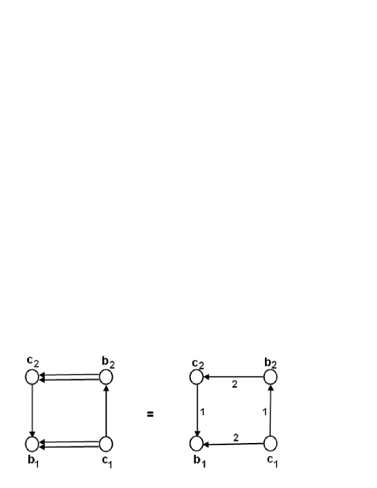
Figure 1: the primitive quiver $\mathfrak{Q}_{0}^{su_{3}}$ made completely of elementary BPS states with central charges in the half plane $\mathcal{H}$.

3) $\mathfrak{Q}_{0}^{su_{3}}$ as a symplectic quiver
From the figure 1, we learn that the graph $\mathfrak{Q}_{0}^{su_{3}}$ is completely specified by the charge vectors $\left(b,c\right)$ and their EM products (45). Moreover, because of the two following features:

• the linear dependence of the central charge into the EM charges of the BPS states,

• the appearance of the pair $\left(b_{i},c_{i}\right)$ of charge vectors as a building block of $\mathfrak{Q}_{0}^{su_{3}}$,

it is natural to group together these charges into a large vector $\mathbf{v}$ having $\left(2r\right)^{2}=16$ components as follow

$$\mathbf{v}_{I}=\left(\begin{array}[]{c}b_{1}\\ b_{2}\\ c_{1}\\ c_{2}\end{array}\right),\qquad r=2$$ (46)

with $b_{i}$ and $c_{i}$ given by eq(35). In this way of doing, the quiver $\mathfrak{Q}_{0}^{su_{3}}$ can be then defined by the above vector $\mathbf{v}_{I}$ together with the antisymmetric intersection matrix $\mathcal{J}_{IJ}=\mathbf{v}_{I}\circ\mathbf{v}_{J}$ which, by using (45), reads as

$$\mathcal{J}_{IJ}=\left(\begin{array}[]{cc}0&-K_{ij}I_{4\times 4}\\ K_{ji}I_{4\times 4}&0\end{array}\right)$$ (47)

with $I_{4\times 4}$ the $4\times 4$ identity matrix and

$$K_{ij}=\left(\begin{array}[]{cc}2&-1\\ -1&2\end{array}\right)$$ (48)

Below, we denote the vector (46) by $\mathbf{v}^{\left(0\right)}$ where the upper index refers to $\mathfrak{Q}_{0}^{su_{3}}$. Later on we will also consider the vectors

$$\mathbf{v}^{\left(n\right)}=\left(\begin{array}[]{c}b_{1}^{\left(n\right)}\\ b_{2}^{\left(n\right)}\\ c_{1}^{\left(n\right)}\\ c_{2}^{\left(n\right)}\end{array}\right),\qquad n\geq 0$$ (49)

describing the mutated BPS quivers $\mathfrak{Q}_{n}^{su_{3}}$ that are related to $\mathfrak{Q}_{0}^{su_{3}}$ by performing $n$ successive elementary mutations.
Notice that the matrix representation (46) of $\mathbf{v}^{\left(0\right)}$ is not unique since it is defined up to permutations of the entries. So there are different, but equivalent, choices of parameterizing the vector $\mathbf{v}^{\left(0\right)}$; each having an advantage and a disadvantage; say a specific feature. For example the choice (46) allows to exhibit explicitly the Cartan matrix in the electric magnetic products as in (47), while the choice

$$\left(\begin{array}[]{c}b_{1}\\ c_{1}\\ b_{2}\\ c_{2}\end{array}\right)$$ (50)

puts in front the $SU\left(2\right)$ building block property of the quiver. In what follows, we consider the parametrization (46-47-49). The choice (50) will be used in section 6 and 7 when considering the weak coupling chamber.

3.2 Quivers, Dynkin graphs and chambers

BPS quivers in the $\mathcal{N}=2$ supersymmetric pure gauge theory with a spontaneously broken gauge symmetry $G$ are intimately linked to the Dynkin graph of $G$ depicted by the figures 3. Moreover, as for Dynkin diagrams of simple Lie algebras, the primitive $\mathfrak{Q}_{0}^{G}$’s of the BPS quiver theory have also outer-automorphism symmetries that can be used other purposes such as approaching the BPS spectra of $\mathcal{N}=2$ QFTs with non simply laced gauge symmetries [31, 32]. As far BPS quivers are concerned, these outer-automorphisms have to commute with the mutation transformations.

3.2.1 Link with Dynkin graphs

The link between BPS quivers and Dynkin graphs of the underlying gauge symmetries of the $\mathcal{N}=2$ supersymmetric QFT is manifested through two channels: either by quiver folding to compensate the orientation of BPS quivers; or by the shared outer-automorphism symmetries.

folding
Quiver folding is direct way to exhibit the link between the BPS quivers of the $\mathcal{N}=2$ QFT and Dynkin diagrams. In the case of the gauge symmetry $SU\left(3\right)$, the link is as depicted in fig 2. There, one first considers two oriented primitive quivers $\mathfrak{Q}_{0}^{su_{3}}$ and $\mathfrak{P}_{0}^{su_{3}}$, with EM charges as follows:

$$\ \ \ \ \mathfrak{Q}_{0}^{su_{3}}$$

(51)

then compensate the quiver orientations by folding the $b_{i},c_{i}$ nodes among themselves; and do the same thing for $b_{i}^{\prime},c_{i}^{\prime}$. As such, the obtained quiver has the following nodes

$$w_{i}=b_{i}+c_{i}$$ ,

(52)

In this way, one ends with two un-oriented diagrams describing the Dynkin graph of $SU\left(3\right)\times SU\left(3\right)$ with gauge particles $w_{i}$ and $w_{i}^{\prime}$.

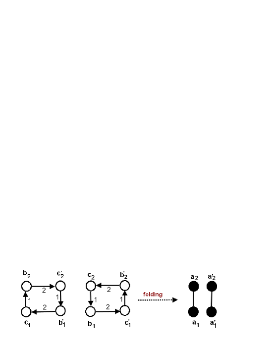
Figure 2: the SU$\left(3\right)$ Dynkin graph obtained by folding the nodes of the BPS quiver $\mathfrak{Q}^{su_{3}}$ interchanged by the outer automorphism $\mathbb{Z}_{2}^{diag}$.

The quiver doubling is the price to pay to kill the orientation. This construction extends to the Dynkin graphs of all ADE Lie algebras.

outer-automorphisms
The BPS Quivers of the supersymmetric broken SU$\left(3\right)$ gauge theory has an outer-automorphism symmetry isomorphic to the outer- automorphism group of the $SU\left(3\right)$ Dynkin graph. Here also this property is not specific for $SU\left(3\right)$; it exists as well for BPS quivers of $\mathcal{N}=2$ QFTs associated with any simply laced gauge symmetry G with Dynkin diagram of $G$ as in fig 3.

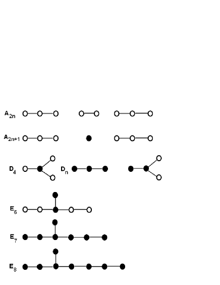
Figure 3: Outer automorphisms of Dynkin graphs; red nodes indicate those simple roots that are fixed by outer-automorphisms.

Notice that the usual outer-automorphism symmetries $\Gamma^{G}$ are very important in gauge theories; they are generally used to approach non simply laced gauge symmetries from the ADE ones; offering therefore a tricky way to get the BPS spectra of $\mathcal{N}=2$ supersymmetric QFTs with non simply laced gauge symmetries [33, 34, 35]. For example, the Dynkin graph of the $SO\left(2N+1\right)$ non simply laced series can be obtained by folding the nodes the Dynkin graph of $SO\left(2N+2\right)$ which are interchanged by the $\mathbb{Z}_{2}$ outer automorphism symmetry. Similarly, the Dynkin graph of G₂ can be obtained by folding three nodes of the SO$\left(4\right)$ graph. In general, the outer automorphism groups $\Gamma^{G}$ for the Dynkin diagrams and the number of fixed of simple roots are as follows.

(60)

and the result on folding is:

$$D_{N+1}/\mathbb{Z}_{2}$$

(61)

case of SU$\left(3\right)$
In the case of BPS quivers of the $SU\left(3\right)$ gauge symmetry, the outer automorphisms act on the $SU\left(3\right)$ Dynkin graph by interchanging its two nodes $\alpha_{1},$ $\alpha_{2}$. On the side of BPS quiver theory, this symmetry corresponds to permuting the role of the two monopoles among themselves and the same thing for the two dyons; this leaves the quiver $\mathfrak{Q}_{0}^{su_{3}}$ invariant.

$$b_{1}$$ and

(62)

At the diagrammatic level, (62) corresponds to rotate the planar quiver $\mathfrak{Q}_{0}^{su_{3}}$ around its central axis by an angle $\pi$ as depicted on the figure 4; this discrete symmetry describes to the equivalence of viewing the quiver from top or from bottom.

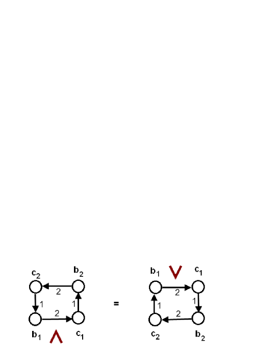
Figure 4: the BPS quiver viewed from top and from bottom.

Using (46), one can represents the action of the outer automorphisms on the nodes of $\mathfrak{Q}_{0}^{su_{3}}$ by a linear representation on the vector $\mathbf{v}^{\left(0\right)}$ that leaves invariant the intersection matrix $\mathcal{A}^{\left(0\right)}$. We have

$$\begin{array}[]{ccc}\mathbf{v}^{\left(0\right)}&\rightarrow&\mathbf{v}^{\prime\left(0\right)}=M_{0}\mathbf{v}^{\left(0\right)}\end{array}$$ (63)

with

$$\mathcal{A}^{\prime\left(0\right)}=M_{0}\mathcal{A}^{\left(0\right)}M_{0}^{T}=\mathcal{A}^{\left(0\right)}$$ (64)

More explicitly,

$$\mathbf{v}^{\prime\left(0\right)}=\left(\begin{array}[]{c}b_{2}\\ b_{1}\\ c_{2}\\ c_{1}\end{array}\right)$$ (65)

from which we read

$$M_{0}=\left(\begin{array}[]{cccc}0&I_{2}&0&0\\ I_{2}&0&0&0\\ 0&0&0&I_{2}\\ 0&0&I_{2}&0\end{array}\right)=M_{0}^{T}$$ (66)

satisfying the properties $M_{0}^{2}=I_{id}$. Then, quivers $\mathfrak{Q}_{n}^{su_{3}}$ that are related under outer automorphism transformations should be identified; so mutation transformations should commute with outer automorphisms.

3.2.2 the cone of BPS particles

A chamber in the quiver theory of [1, 2] contains many BPS states organized into several packages of BPS states belonging to several quivers related among themselves by mutation transformations.
In the case of $SU\left(3\right)$ gauge symmetry, the BPS states belonging to a chamber are arranged into subsets of 4 BPS states each; related by mutation transformations. To build a chamber in the $SU\left(3\right)$ BPS quiver theory, one proceeds as follows:

• start with 4 BPS particles with EM charges $\vec{\gamma}_{1},$ $\vec{\gamma}_{2},$ $\vec{\gamma}_{3},$ $\vec{\gamma}_{4}$ and intersection matrix $\mathcal{J}_{ij}=\vec{\gamma}_{i}\circ\vec{\gamma}_{j}$ and central charges $Z_{i}=Z\left(\vec{\gamma}_{i}\right)$.

• think about the complex numbers $Z_{i}$ as points in the complex plane $Z\sim\left(\mathop{\mathrm{R}e}Z,\mathop{\mathrm{I}m}Z\right)$ with absolute values $\left|Z_{i}\right|$ giving the masses $m_{\gamma_{i}}$ of the BPS particles and the arguments $\arg Z_{i}$ to make partial ordering from left to right or equivalently from right to left in the upper half plane $\mathop{\mathrm{I}m}Z>0$; see fig 5.

  

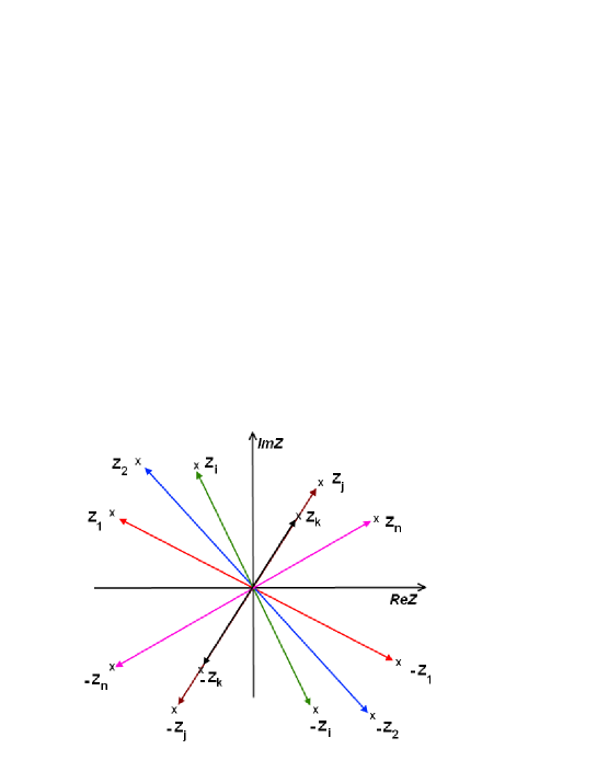
  Figure 5: Central charges of BPS and anti-BPS states as points in the complex $Z$ plane.

  In general there are several ways to order these arguments as given by the cone,

  $$\pi>\arg Z_{i_{1}}>\arg Z_{i_{2}}>\arg Z_{i_{3}}>\arg Z_{i_{4}}>0$$ (67)

• introduce the vectors $\mathbf{v}^{\left(0\right)}$ and $\Theta^{\left(0\right)}$

  $$\mathbf{v}^{\left(0\right)}=\left(\begin{array}[]{c}\vec{\gamma}_{1}\\ \vec{\gamma}_{2}\\ \vec{\gamma}_{3}\\ \vec{\gamma}_{4}\end{array}\right)$$ ,

  (68)

  with no matter about the order of the entries of $\mathbf{v}^{\left(0\right)}$. Then perform mutations of BPS quivers which, in this set up, are realized by linear transformations of these vectors as follows

  $$\mathbf{v}^{\left(0\right)}\rightarrow$$

  (69)

The BPS chamber is finite if the above sequence of mutations is finite; otherwise it is infinite. In what follows, we will take the 4 initial BPS particles as given by the two elementary monopoles $\mathfrak{M}_{i}$ and the two elementary dyons $\mathfrak{D}_{i}$ with respective EM charges $b_{i}$ and $c_{i}$; and central charges as

$$Z\left(b_{i}\right)=X_{i}$$ ,

(70)

We also have

$$\mathbf{v}^{\left(0\right)}=\left(\begin{array}[]{c}b_{1}\\ b_{2}\\ b_{1}\\ b_{2}\end{array}\right)$$ ,

(71)

Notice that because of the ordering of the states is partial; then one may have several BPS particles that have different masses $\left|Z_{i_{1}}\right|\neq...\neq\left|Z_{i_{4}}\right|$; but with the same angle arg$Z_{i_{1}}=...=\arg Z_{i_{4}}$. For illustration see the example of the two BPS particles $Z_{j}$ and $Z_{k}$ of fig 5. Obviously these BPS particles corresponds to different nodes in the quiver as the multiplicity of these hypermultiplets is equal to one. This feature has an interpretation in terms of commuting basis reflections as given by eqs (122-123), see also fig 16 reported in appendix I; it will be used when building the strong coupling chamber of ADE gauge theories.

• BPS and anti- BPS states
  The angle $\arg Z_{u}$ can take values in the interval $\left[0,2\pi\right]$, the complex $Z$ plane of the central charges at a point $u$ is divided into two half planes:

  $$\mathcal{H}_{u}^{+}=\left\{\mathop{\mathrm{I}m}Z>0\right\}$$ and

  (72)

  In the upper half plane $\mathcal{H}_{u}^{+}\equiv\mathcal{H}_{u}$ lives the BPS particles and are partially ordered according to $0<\arg Z_{u}<\pi$ while in the half plane $\mathcal{H}_{u}^{-}$ lives the anti-BPS states and we have $\pi<\arg Z_{u}<2\pi.$ The total BPS spectrum is given by all states that live on the full plane $\mathcal{H}_{u}$ of central charges; and so this spectrum is CPT invariant.
  

• left most and right most BPS states

  By using $\arg Z_{u}$, the partial ordering of the central charges $Z_{u}\left(\gamma_{i}\right)\equiv Z_{i}$ in $\mathcal{H}_{u}$ allows to distinguish several sequences depending on the angles of the central charges. A typical sequence of $l$ BPS particles is given by (67) where $Z_{i_{1}}$ appears at left most, $Z_{i_{2}}$ the second left one and so on.
  We also have $Z_{i_{4}}$ the right most BPS, $Z_{i_{3}}$ the next right one an so on. The knowledge of (67) is important for choosing the BPS state to begin with in performing quiver mutations.

4 Strong coupling chambers in $SU\left(N\right)$ theories

In this section, we study the isotropy group structure of the set $\mathcal{G}_{strong}^{su_{N}}$ of mutation transformations of the BPS quivers of $\mathcal{N}=2$ supersymmetric quantum field theories with $SU\left(N\right)$ gauge symmetry and use this mutation group to build the BPS spectra of the strong coupling chambers. To see how the machinery works, we begin by studying the leading cases $N=2,3,4$; then we give the general result for the $SU\left(N\right)$ series. The $\mathcal{N}=2$ supersymmetric QFT’s with $SO\left(2N\right)$ and $E_{r}$ gauge symmetries will be considered in section 5.

4.1 $SU\left(2\right)$ theory

This is a particular model that has been studied explicitly in [1, 2]; see also [10, 11, 12, 13, 19]. Here, we reconsider this theory by using a groupoid approach. This study is useful as it allows to get more insight into BPS quiver theory associated with higher dimensional gauge symmetries.
The strong coupling chamber of the effective 4D $\mathcal{N}=2$ supersymmetric pure SU$\left(2\right)$ gauge theory has $2$ BPS states and $2$ anti-BPS ones. These are:

• a monopole $\mathfrak{M}$ and a dyon $\mathfrak{D}$ with respective EM charge $b,$ $c$; and respective complex central charges $X$ and $Y$;

• their CPT conjugate $\mathfrak{\bar{M}}$ and $\mathfrak{\bar{D}}$ having opposite EM charge; i.e: $-b,$ $-c$.

In terms of the arguments of the central charges, the BPS states of the strong coupling chamber of this gauge theory corresponds to

$$\arg Y>\arg X$$ (73)

The content of this chamber can be explicitly derived by applying the quiver mutation method of [1, 2] which is illustrated on fig 6

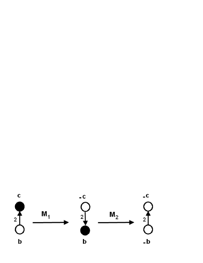
Figure 6: Strong coupling chamber using mutations of the primitive quiver $\mathfrak{Q}_{0}^{su_{2}}$

From these quiver mutations, it follows that the transformations $\mathcal{M}_{0,n}$ can be realized on the EM charge vector $v=\left(b,c\right)$ as linear mappings generated by two matrices $L_{1}$ and $L_{2}$ as follows

$$L_{1}=\left(\begin{array}[]{cc}1&0\\ 0&-1\end{array}\right)$$ ,

(74)

Notice that $L_{1}=-L_{2}=L$, this is a very particular feature that is specific for SU$\left(2\right)$ and has no analogue for the case of higher dimensional gauge symmetry. We also have the properties

$$\left(L_{1}\right)^{2}=\left(L_{2}\right)^{2}=I_{id}$$ (75)

and

$$\left(L_{i}L_{j}\right)^{m_{ij}}=I_{id}$$ (76)

with $m_{ij}$ the entries of the following integral $2\times 2$ symmetric matrix

$$M=\left(\begin{array}[]{cc}1&2\\ 2&1\end{array}\right)$$ (77)

The relations (75-76-77) turns out to play a crucial role in the study of the symmetry structure of mutation transformations in the BPS quiver theory. They encode a general result that is valid for all ADE gauge symmetries of the BPS quiver theory. 
By using the two generators $L_{1}$ and $L_{2}$, it is not difficult to check that a generic quiver mutation mapping $\mathfrak{Q}_{0}^{su_{2}}$ into $\mathfrak{Q}_{n}^{su_{2}}$ depends on the parity of the positive integer $n$. We have

$$\mathcal{M}_{2k}$$

(78)

However, since $\left(L_{i}\right)^{2}=I_{id}$, it follows that the set of mutations form a finite dimensional group that we denote as $\mathcal{G}_{strong}^{su_{2}}$. This group has 4 elements namely $\left\{I_{id},+L,-I_{id},-L\right\}$; and which, for later use, we prefer to write as follows

$$\mathcal{G}_{strong}^{su_{2}}$$

(79)

or equivalently like

$$\mathcal{G}_{strong}^{su_{2}}$$

(80)

We also have the following identities useful for generalization to higher dimensional gauge symmetries

$$\left(L_{2}L_{1}\right)^{2}$$ ,

,

(81)

and

$$L_{2}L_{1}$$

(82)

The multiplication table of the mutation group $\mathcal{G}_{M}^{su_{2}}$ is as follows

$$\mathcal{G}_{M}^{su_{2}}$$

(83)

Notice that the order of this discrete group is

$$\text{order}\left(\mathcal{G}_{strong}^{su_{2}}\right)=\left|\mathcal{G}_{strong}^{su_{2}}\right|=4$$ (84)

it is precisely the number of BPS states and anti-BPS states in the strong coupling chamber. For later use think about this number as

$$\#_{bsp+antibps}=\left|\mathcal{G}_{strong}^{su_{2}}\right|\times r$$ (85)

with $r$ the rank of $SU\left(2\right)$. Below, we give the extension of this matrix mutation group construction for the cases of $SU\left(3\right)$ and $SU\left(4\right)$ models; the generalization to the generic $SU\left(N\right)$ gauge groups will be reported in appendix II.

4.2 $SU\left(3\right)$ model

Following [1, 2], the strong coupling chamber of the $\mathcal{N}=2$ supersymmetric pure $SU\left(3\right)$ gauge theory has 6 BPS states and 6 anti-BPS ones. These states can be obtained by performing mutations of $\mathfrak{Q}_{0}^{su_{3}}$. Below, we use our algebraic method to get the full set of BPS states of the strong coupling chamber. This approach relies on building the family of mutated quivers $\mathfrak{Q}_{n}^{su_{3}}$ in the strong coupling chamber by using $\mathcal{G}_{strong}^{su_{3}}$.

4.2.1 The $\mathfrak{Q}_{n}^{su_{3}}$ quiver family

First, consider the primitive quiver $\mathfrak{Q}_{0}^{su_{3}}$ given by the graph (1); this quiver is associated with a point $\left(u_{1},u_{2}\right)$ of the Coulomb branch of the moduli space of the theory; and involves only elementary BPS states. In our approach, the quiver $\mathfrak{Q}_{0}^{su_{3}}$ is represented by the two following:
(i) the $\left(2r\right)^{2}$ component vector with $r=2$; the rank of $SU\left(3\right)$,

$$\mathbf{v}^{\left(0\right)}=\left(\begin{array}[]{c}b_{1}\\ b_{2}\\ c_{1}\\ c_{2}\end{array}\right)$$ (86)

this vector combines the EM vector charges of the 4 elementary BPS states.
(ii) the intersection matrix

$$\mathcal{A}_{IJ}^{\left(0\right)}=\mathbf{v}_{I}^{\left(0\right)}\circ\mathbf{v}_{J}^{\left(0\right)}.$$ (87)

given by eq(47).

To get the expressions of the remaining BPS states of the strong coupling chamber, we have to perform successive mutations of $\mathfrak{Q}_{0}^{su_{3}}$ until reaching the quiver $\mathfrak{Q}_{0}^{su_{3}}$ again. The mutations are by the following reflections,

$$\gamma_{i}^{\prime}$$

if

if

(88)

with the integers $N_{ji}=\gamma_{j}\circ\gamma_{i}$ given by eqs(45-47).
In what follows, we use the groupoid method to derive the explicit BPS content of the strong coupling chamber. The method is as follows:
(1) describe the generic BPS quivers $\mathfrak{Q}_{n}^{su_{3}}$ of the strong coupling chamber by the vector

$$\mathbf{v}^{\left(n\right)}=\left(\begin{array}[]{c}b_{1}^{\left(n\right)}\\ b_{2}^{\left(n\right)}\\ c_{1}^{\left(n\right)}\\ c_{2}^{\left(n\right)}\end{array}\right),\qquad n=0,1,2,...$$ (89)

with entries describing the nodes of the quiver and intersections $\mathcal{A}_{IJ}^{\left(n\right)}=\mathbf{v}_{I}^{\left(n\right)}\circ\mathbf{v}_{J}^{\left(n\right)}$ as

$$\mathcal{A}_{IJ}^{\left(n\right)}=\left(\begin{array}[]{cc}0&b_{i}^{\left(n\right)}\circ c_{j}^{\left(n\right)}\\ c_{i}^{\left(n\right)}\circ b_{j}^{\left(n\right)}&0\end{array}\right)$$ (90)

In this view, $\mathfrak{Q}_{0}^{su_{3}}$ appears precisely as the leading member of the family

$$\mathbb{B}_{strong}^{su_{3}}=\left\{\mathfrak{Q}_{n}^{su_{3}};\text{ }n\geq 0\right\}.$$ (91)

which should be thought of as the base of objects in groupoid langauge.
(2) interpret $b_{i}^{\left(n\right)}$ and $c_{i}^{\left(n\right)}$ as the EM charge vectors of BPS states of the strong coupling chamber. We also have $b_{i}^{\left(0\right)}=b_{i}$ and $c_{i}^{\left(0\right)}=c_{i}$.
The same feature holds for the central charges $X_{i}^{\left(n\right)}$ and $Y_{i}^{\left(n\right)}$ of the BPS states

$$X_{i}^{\left(n\right)}=Z(b_{i}^{\left(n\right)})$$ ,

(92)

(3) think about the mutation from $\mathfrak{Q}_{0}^{su_{3}}$ to $\mathfrak{Q}_{n}^{su_{3}}$ as a linear mapping of $\mathbf{v}^{\left(0\right)}$ into $\mathbf{v}^{\left(n\right)}$ like,

$$\mathbf{v}^{\left(n\right)}=\mathcal{M}_{0}\mathbf{v}^{\left(0\right)},\qquad n=0,1,2,...$$ (93)

with

$$\mathcal{M}_{0}=I_{id}$$

and the mutations $\mathcal{M}_{0}$ given by some matrices of $GL\left(4,\mathbb{Z}\right)$ that we have to determine. These matrices are obtained by using the iteration property

$$\mathbf{v}^{\left(n\right)}=L_{n}\mathbf{v}^{\left(n-1\right)},\qquad n=1,2,...$$ (94)

leading to the realization

$$\mathcal{M}_{n}=L_{n}L_{n-1}...L_{2}L_{1}=\mathop{\displaystyle\prod}\limits_{k=1}^{n}L_{n+1-k}$$ (95)

and showing that the $\mathcal{M}_{n}$’s (thought of as $\mathcal{M}_{n,0}$) are particular groupoid morphisms of $\mathbb{G}_{su_{3}}$ acting on the BPS chambers $\mathbb{B}_{su_{3}}$

$$\mathbb{G}_{su_{3}}=\left\{\mathcal{M}_{n,m}:\mathfrak{Q}_{m}^{su_{3}}\rightarrow\mathfrak{Q}_{n}^{su_{3}},\qquad\mathfrak{Q}_{k}^{su_{3}}\in\mathbb{B}_{su_{3}}\right\}$$ (96)

with the binary composition as in appendix I; eq(358).
(4) To deal with (95), one has to identify the appropriate ordering of the arguments of the complex central charges $X_{i}$ and $Y_{i}$ of the two monopoles and the two dyons that make $\mathfrak{Q}_{0}^{su_{3}}$. It happens that the adequate choice that leads to the BPS spectrum of the strong coupling chamber corresponds to

$$\arg Y_{1}$$

(97)

and

$$\arg Y_{i}>\arg X_{i}$$ .

(98)

The relations (97) teach us that one has to treat on equal footing the two dyons and the same thing for the two monopoles; a helpful property which will be interpreted later and that will be used below.

4.2.2 Building the $\mathfrak{Q}_{n}^{su_{3}}$’s of the chamber $\arg Y>\arg X$

To get the family of mutated quivers $\mathfrak{Q}_{n}^{su_{3}}$ of the chamber $\arg Y>\arg X$, we use the property that the order of this chamber is finite. Denote this order by the positive integer as $n_{0}$; and proceeds as follows:

• first, mutate simultaneously the two nodes $c_{i}^{\left(0\right)}=c_{i}$ associated with the two dyons having central charges $Y_{i}$. This collective operation, which is represented by the mutation matrix $L_{1}$, leads to the quiver $\mathfrak{Q}_{1}^{su_{3}}$ made of two nodes $b_{i}^{\left(1\right)}$ and two nodes $c_{i}^{\left(1\right)}$ related by the intersection matrix $b_{i}^{\left(1\right)}\circ c_{j}^{\left(1\right)}$. Using eqs(89-90), we have

  $$v_{I}^{\left(1\right)}$$

  (99)

  or in a condensed manner like

  $$v^{\left(1\right)}$$

  (100)

  Therefore $L_{1}$ specifies completely the BPS quiver $\mathfrak{Q}_{1}^{su_{3}}$. Notice that due to $\left(L_{1}\right)^{2}=I_{id}$ we have the following inverse mutation

  $$v^{\left(0\right)}$$

  (101)

• second, mutate simultaneously the two nodes $b_{i}^{\left(1\right)}$ of the quiver $\mathfrak{Q}_{1}^{su_{3}}$ to end with a mutated quiver $\mathfrak{Q}_{2}^{su_{3}}$ with two nodes $b_{i}^{\left(2\right)}$ and two $c_{i}^{\left(2\right)}$ and intersection matrix $b_{i}^{\left(2\right)}\circ c_{i}^{\left(2\right)}$. Using the convention notations (89-90), we have

  $$v^{\left(2\right)}$$

  (102)

  with $\mathcal{M}_{2}$ as in (95) and similar relations to (101).

• continue the mutation operations until reaching the quiver $\mathfrak{Q}_{n_{0}-1}^{su_{3}}$ made of the two nodes $b_{i}^{\left(n_{0}-1\right)}$ and the two $c_{i}^{\left(n_{0}-1\right)}$. The mutation relations are then as follows

  $$v^{\left(n_{0}-1\right)}$$

  (103)

  or equivalently

  $$v^{\left(n_{0}-1\right)}$$

  (104)

• Because of the property of finite chamber order, the next mutation should lead to the identity; then the quiver $\mathfrak{Q}_{n_{0}}^{su_{3}}$ made by the two nodes $b_{i}^{\left(n_{0}\right)}$ and the two nodes $c_{i}^{\left(n_{0}\right)}$ has to coincide with the primitive $\mathfrak{Q}_{0}^{su_{3}}$. We have

  $$v^{\left(n_{0}\right)}$$

  (105)

  with

  $$v^{\left(n_{0}\right)}$$

  (106)

  We also have

  $$v^{\left(n_{0}\right)}$$

  with the following constraint relation of the mutation matrices

  $$\mathcal{M}_{n_{0}}=L_{n_{0}}L_{n_{0}-1}...L_{2}L_{1}=I_{id}$$ (107)

4.3 Building the mutation set $\mathcal{G}_{strong}^{su_{3}}$

We begin by analyzing eqs (97) which we use it to build the mutation set $\mathcal{G}_{strong}^{su_{3}}$. Then we work out the 5 possible mutations of the quiver $\mathfrak{Q}_{0}^{su_{3}}$ after what we give the results.

4.3.1 Consequence of eqs (97)

Because of the constraint relations (97), the mutations of $\mathfrak{Q}_{0}^{su_{3}}$ obey the remarkable periodicity property,

$$L_{2n+1}=L_{1}$$ , ,

(108)

It happens that this property is valid for the BPS quivers of any ADE gauge symmetry; and leads to tremendous simplifications. Let us illustrate below how this works for the case of SU$\left(3\right)$. Putting (108) back into (240), we find that the set of matrices $\mathcal{M}_{n}$ is completely generated by $L_{1}$ and $L_{2}$ as given by the following relations

$$\mathcal{M}_{2k}$$

(109)

with $L_{1}$ and $L_{2}$ obeying

$$\left(L_{1}\right)^{2}=\left(L_{2}\right)^{2}=I_{id},$$ (110)

as well as the identities

$$\left(L_{2}L_{1}\right)^{3}$$

(111)

and

$$L_{1}L_{2}L_{1}=L_{2}L_{1}L_{2}$$ (112)

By help of these relations, one can check that the set of BPS quiver mutations (109) form indeed a finite discrete group $\mathcal{G}_{strong}^{su_{3}}$ with order

$$\left|\mathcal{G}_{strong}^{su_{3}}\right|=6$$ (113)

The binary multiplication table of $\mathcal{G}_{strong}^{su_{3}}$ is given by

$$\mathcal{G}_{M}^{su_{3}}$$

(114)

To get more insight into this discrete symmetry group, it is interesting to use Coxeter group formulation, reported in appendix C, by considering: (a) the $2\times 2$ symmetric matrix M with positive integer entries $m_{ij}$ as follows

$$M=\left(\begin{array}[]{cc}1&3\\ 3&1\end{array}\right)$$ (115)

and (b) the finite set

$$W\left(M\right)=\left\langle\left.\begin{array}[]{c}\\ \\ \end{array}\right.L_{1},L_{2}|\text{ }\left(L_{i}L_{j}\right)^{m_{ij}}=I_{id}\right\rangle$$ (116)

from which one recognizes that $\mathcal{G}_{strong}^{su_{3}}$ is nothing but the matrix the Coxeter group $Dih_{6}$ with Coxeter graph isomorphic to the Dynkin diagram of the $SU\left(3\right)$ Lie algebra. The $Dih_{6}$ is a discrete group having 6 elements; it is a particular group of the family $Dih_{2n}$ describing the 2n symmetries consisting of n rotations and n reflections of a regular polygon with n sides.

4.3.2 Computing the BPS spectrum and realizing $\mathcal{G}_{M}^{su_{3}}\simeq Dih_{6}$

Here we compute explicitly the BPS states of the strong coupling chamber of the supersymmetric spontaneously broken $SU\left(3\right)$ gauge theory. We also give the matrix realization of the mutation group $\mathcal{G}_{strong}^{su_{3}}$

$i)$ building the Quiver $\mathfrak{Q}_{1}^{su_{3}}$
To get the mutated BPS quiver $\mathfrak{Q}_{1}^{su_{3}}$ with electric magnetic vector $\boldsymbol{v}^{\left(1\right)}=(\boldsymbol{b}^{\left(1\right)},\boldsymbol{c}^{\left(1\right)})$, we have to mutate simultaneously the charge vectors of the two dyons $c_{1}$ and $c_{2}$. By using the mutation rules, we get the following charge vectors

$$\left(\begin{array}[]{c}b_{1}^{\left(1\right)}\\ b_{2}^{\left(1\right)}\\ c_{1}^{\left(1\right)}\\ c_{2}^{\left(1\right)}\end{array}\right)=\left(\begin{array}[]{c}b_{1}+c_{2}\\ b_{2}+c_{1}\\ -c_{1}\\ -c_{2}\end{array}\right)$$ (117)

from which we can learn the mutation matrix $L_{1}\equiv\mathcal{M}_{1}$ that relates $\boldsymbol{v}^{\left(1\right)}$ and $v^{\left(0\right)}$,

$$L_{1}=\left(\begin{array}[]{cccc}I_{4}&0&0&I_{4}\\ 0&I_{4}&I_{4}&0\\ 0&0&-I_{4}&0\\ 0&0&0&-I_{4}\end{array}\right)$$ (118)

where $I_{4}$ stands for the $4\times 4$ identity matrix. Notice that the rows of $L_{1}$ give precisely the EM charge vectors of the BPS states of the quiver $\mathfrak{Q}_{1}^{su_{3}}$. Notice also that being a triangular matrix, we have

$$\left(L_{1}\right)^{2}=I_{16},\qquad\det L_{1}=1$$ (119)

To get the intersection matrix $\mathcal{A}^{\left(1\right)}$, we use the relation

$$\mathcal{A}^{\left(1\right)}=L_{1}\mathcal{A}^{\left(0\right)}L_{1}^{T}$$ (120)

with

$$\mathcal{A}^{\left(0\right)}=\left(\begin{array}[]{cccc}0&0&2&-1\\ 0&0&-1&2\\ -2&1&0&0\\ 1&-2&0&0\end{array}\right)$$ (121)

Straightforward calculations give $\mathcal{A}^{\left(1\right)}=-\mathcal{A}^{\left(0\right)}.$ Before proceeding notice that being a reflection, one would expect to have $\det L_{1}$ equals to $-1$; but it is not. The point is that $L_{1}$ is not a fundamental reflection, it is the composition of two commuting reflections as,

$$L_{1}=s_{1}t_{1}=t_{1}s_{1}$$ (122)

with

$$s_{1}=\left(\begin{array}[]{cccc}I_{4}&0&0&0\\ 0&I_{4}&I_{4}&0\\ 0&0&-I_{4}&0\\ 0&0&0&I_{4}\end{array}\right)$$ ,

(123)

This feature is also valid for the generator $L_{2}$ which should be thought as $L_{2}=s_{2}t_{2}$. This property is general; it is also valid for higher dimensional ADE gauge symmetries to be considered later on.

$ii)$ the Quiver $\mathfrak{Q}_{2}^{su_{3}}$
To get the BPS quiver $\mathfrak{Q}_{2}^{su_{3}}$, we have to mutate simultaneously the charge vectors $b_{1}^{\left(1\right)}$ and $b_{2}^{\left(1\right)}$ of the quiver $\mathfrak{Q}_{1}^{su_{3}}$. We end with a new charge vector $\boldsymbol{v}^{\left(2\right)}$ with the following components

$$\left(\begin{array}[]{c}b_{1}^{\left(2\right)}\\ b_{2}^{\left(2\right)}\\ c_{1}^{\left(2\right)}\\ c_{2}^{\left(2\right)}\end{array}\right)=\left(\begin{array}[]{c}-b_{1}-c_{2}\\ -b_{2}-c_{1}\\ b_{2}\\ b_{1}\end{array}\right)$$ (124)

This EM charge vector $\boldsymbol{v}^{\left(2\right)}$ is related to $v^{\left(1\right)}$ by the mutation matrix $L_{2}$ given by

$$L_{2}=\left(\begin{array}[]{cccc}-I_{4}&0&0&0\\ 0&-I_{4}&0&0\\ 0&I_{4}&I_{4}&0\\ I_{4}&0&0&I_{4}\end{array}\right),$$ (125)

with

$$\boldsymbol{v}^{\left(2\right)}=L_{2}v^{\left(1\right)}$$ (126)

and, up on using $\boldsymbol{v}^{\left(1\right)}=L_{1}v^{\left(0\right)}$, we also have

$$\boldsymbol{v}^{\left(2\right)}=L_{2}L_{1}v^{\left(0\right)}\equiv\mathcal{M}_{2}v^{\left(0\right)}$$ (127)

Like for $L_{1}$, the matrix $L_{2}$ obeys as well $\left(L_{2}\right)^{2}=I_{16}$; we also have

$$L_{2}=s_{2}t_{2}=t_{2}s_{2}$$ (128)

with

$$s_{2}=\left(\begin{array}[]{cccc}-I_{4}&0&0&0\\ 0&I_{4}&0&0\\ 0&0&I_{4}&0\\ I_{4}&0&0&I_{4}\end{array}\right)$$ ,

(129)

By combining the two successive mutations $L_{1}$ and $L_{2}$, we get the mutation matrix $\mathcal{M}_{2}=L_{2}L_{1}$ that maps the quiver $\mathfrak{Q}_{0}^{su_{3}}$ into the mutated $\mathfrak{Q}_{2}^{su_{3}}$:

$$\mathcal{M}_{2}=\left(\begin{array}[]{cccc}-I_{4}&0&0&-I_{4}\\ 0&-I_{4}&-I_{4}&0\\ 0&I_{4}&0&0\\ I_{4}&0&0&0\end{array}\right)$$ (130)

The EM charges of the BPS and anti-BPS states of this quiver are directly read from the rows of this matrix. We have

$$\mathfrak{Q}_{2}^{su_{3}}:\begin{tabular}[]{lll}$-\left(b_{1}+c_{2}\right)$&,&$b_{2}$\\ $-\left(b_{2}+c_{1}\right)$&,&$b_{1}$\end{tabular}$$ (131)

The intersection matrix is given by

$$\mathcal{A}^{\left(2\right)}=\mathcal{M}_{2}\mathcal{A}^{\left(0\right)}\mathcal{M}_{2}^{T}=\mathcal{A}^{\left(0\right)}$$ (132)

$iii)$ the quiver $\mathfrak{Q}_{3}^{su_{3}}$
Using the property (95), the BPS quiver $\mathfrak{Q}_{3}^{su_{3}}$ is given by

$$\boldsymbol{v}^{\left(3\right)}=\mathcal{M}_{3}v^{\left(0\right)}$$ ,

(133)

with

$$\mathcal{M}_{3}=\left(\begin{array}[]{cccc}0&0&0&-I_{4}\\ 0&0&-I_{4}&0\\ 0&-I_{4}&0&0\\ -I_{4}&0&0&0\end{array}\right)$$ (134)

and

$$\left(\begin{array}[]{c}b_{1}^{\left(3\right)}\\ b_{2}^{\left(3\right)}\\ c_{1}^{\left(3\right)}\\ c_{2}^{\left(3\right)}\end{array}\right)=\left(\begin{array}[]{c}-c_{2}\\ -c_{1}\\ -b_{2}\\ -b_{1}\end{array}\right)$$ (135)

We also have $\mathcal{A}^{\left(3\right)}=\mathcal{M}_{3}\mathcal{A}^{\left(0\right)}\mathcal{M}_{3}^{T}$ $=-\mathcal{A}^{\left(0\right)}$.

$iv)$ the quiver $\mathfrak{Q}_{4}^{su_{3}}$
the BPS quiver $\mathfrak{Q}_{4}^{su_{3}}$ is described by

$$\boldsymbol{v}^{\left(4\right)}$$

(136)

with

$$\mathcal{M}_{4}=\left(\begin{array}[]{cccc}0&0&0&I_{4}\\ 0&0&I_{4}&0\\ 0&-I_{4}&-I_{4}&0\\ -I_{4}&0&0&-I_{4}\end{array}\right),\qquad\mathcal{M}_{4}=\left(\mathcal{M}_{2}\right)^{2}$$ (137)

From this mutation matrix, we learn the electric-magnetic charges of the quiver. We have

$$\left(\begin{array}[]{c}b_{1}^{\left(4\right)}\\ b_{2}^{\left(4\right)}\\ c_{1}^{\left(4\right)}\\ c_{2}^{\left(4\right)}\end{array}\right)=\left(\begin{array}[]{c}c_{2}\\ c_{1}\\ -b_{2}-c_{1}\\ -b_{1}-c_{2}\end{array}\right)$$ (138)

$v)$ the quiver $\mathfrak{Q}_{5}^{su_{3}}$
the BPS quiver $\mathfrak{Q}_{5}^{su_{3}}$ is given by

$$\boldsymbol{v}^{\left(5\right)}$$

(139)

with $\mathcal{M}_{5}=L_{1}\left(\mathcal{M}_{2}\right)^{2}$ as

$$\mathcal{M}_{5}=\left(\begin{array}[]{cccc}-I_{4}&0&0&0\\ 0&-I_{4}&0&0\\ 0&I_{4}&I_{4}&0\\ I_{4}&0&0&I_{4}\end{array}\right)$$ (140)

The corresponding BPS states are

$$\left(\begin{array}[]{c}b_{1}^{\left(5\right)}\\ b_{2}^{\left(5\right)}\\ c_{1}^{\left(5\right)}\\ c_{2}^{\left(5\right)}\end{array}\right)=\left(\begin{array}[]{c}-b_{1}\\ -b_{2}\\ b_{2}+c_{1}\\ b_{1}+c_{2}\end{array}\right)$$ (141)

$vi)$ the quiver $\mathfrak{Q}_{6}^{su_{3}}$
the BPS quiver $\mathfrak{Q}_{6}^{su_{3}}$ is given by the charge vector $\boldsymbol{v}^{\left(6\right)}$ and the intersection matrix $\mathcal{A}^{\left(6\right)}$

$$\boldsymbol{v}^{\left(6\right)}=\mathcal{M}_{6}v^{\left(0\right)}$$ ,

(142)

with $\mathcal{M}_{6}=\left(\mathcal{M}_{2}\right)^{3}$ as

$$\mathcal{M}_{6}=\left(\begin{array}[]{cccc}I_{4}&0&0&0\\ 0&I_{4}&0&0\\ 0&0&I_{4}&0\\ 0&0&0&I_{4}\end{array}\right)$$ (143)

The BPS states are given by

$$\left(\begin{array}[]{c}b_{1}^{\left(6\right)}\\ b_{2}^{\left(6\right)}\\ c_{1}^{\left(6\right)}\\ c_{2}^{\left(6\right)}\end{array}\right)=\left(\begin{array}[]{c}b_{1}\\ b_{2}\\ c_{1}\\ c_{2}\end{array}\right)$$ (144)

and are precisely the BPS states of the primitive quiver $\mathfrak{Q}_{0}^{su_{3}}$. The various steps of the mutations are illustrated on fig 7.

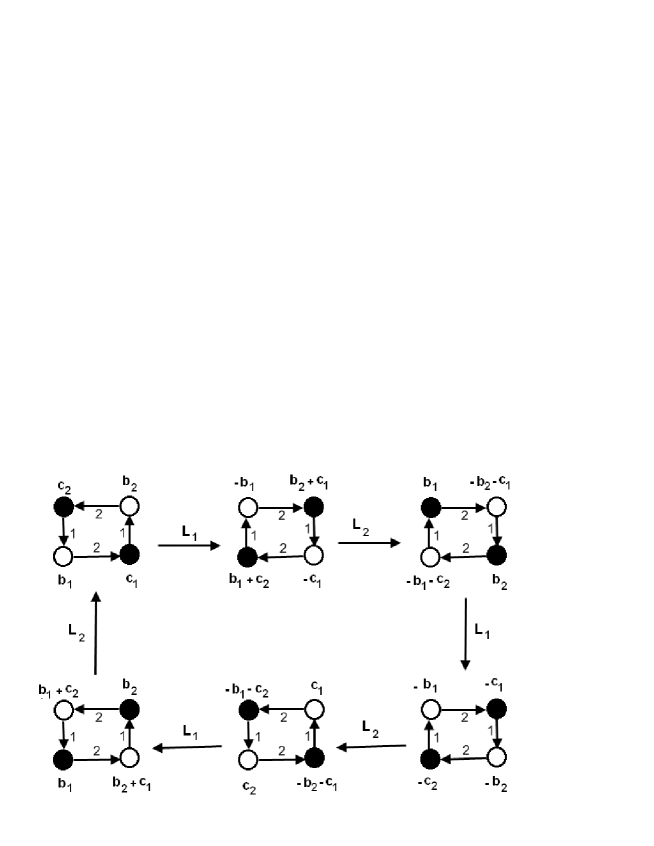
Figure 7: Mutations of the quiver $\mathfrak{Q}_{0}^{su_{3}}$ of pure supersymmetric SU$\left(3\right)$ gauge theory

We conclude this subsection by the following summary:

1) the $\mathfrak{Q}_{n}^{su_{3}}$ quivers
Generic quivers $\mathfrak{Q}_{n}^{su_{3}}$ describing BPS states in the strong coupling chamber of the $\mathcal{N}=2$ QFT₄ with spontaneously broken $SU\left(3\right)$ gauge symmetry are completely characterized by the $\left(v^{\left(0\right)},\mathcal{A}^{\left(0\right)}\right)$ and the mutation group $\mathcal{G}_{strong}^{su_{3}}$. The entries of $v^{\left(n\right)}$ and the intersection matrix are as

$$\begin{tabular}[]{ll}$v^{\left(n\right)}$&$=\left(\begin{array}[]{c}b^{\left(n\right)}\\ c^{\left(n\right)}\end{array}\right)$\\ $\mathcal{A}^{\left(n\right)}$&$=v^{\left(n\right)}\circ v^{\left(n\right)}$\end{tabular},\qquad n=0,...,5$$ (145)

with

$$b^{\left(n\right)}=\left(\begin{array}[]{c}b_{1}^{\left(n\right)}\\ b_{2}^{\left(n\right)}\end{array}\right)$$ ,

(146)

2) BPS spectrum
The BPS states of the strong coupling chamber are given by supersymmetric BPS states with EM charge vectors as follows

$$\pm b_{1}$$ , ,

, ,

(147)

The number of the BPS and anti-BPS states is twice the order of the group of mutation transformations $\mathcal{G}_{strong}^{su_{3}}$ which is isomorphic to the order 6 dihedral Coxeter group

$$\mathcal{G}_{strong}^{su_{3}}\simeq Dih_{6}$$ (148)

3) structure of $\mathcal{G}_{strong}^{su_{3}}$
The matrix mutations $\mathcal{M}_{n}$ map the primitive $\mathfrak{Q}_{0}^{su_{3}}$ into $\mathfrak{Q}_{n}^{su_{3}}$. These mutations, which can be learnt from eqs(118-144), are invertible and form a discrete group $\mathcal{G}_{strong}^{su_{3}}$ with elements

$$\mathcal{M}_{1},$$

(149)

These elements obey a set of properties; in particular

$$\mathcal{M}_{n+6}=\mathcal{M}_{n},\qquad\left(\mathcal{M}_{2}\right)^{3}=I_{16}$$ (150)

as well as

$$\mathcal{M}_{3}=\mathcal{M}_{1}\mathcal{M}_{2}$$ ,

,

(151)

leading to the group multiplication table (114). Notice moreover that the generators $L_{1}$ and $L_{2}$ play a symmetric role as exhibited by the following identities

$$\mathcal{M}_{1}=L_{1}$$ ,

,

(152)

and

$$\mathcal{M}_{3}=L_{1}L_{2}L_{1}=L_{2}L_{1}L_{2}$$ (153)

This property captures the fact that one needs both left and right mutations to build the BPS chamber.

4.4 $SU\left(4\right)$ model

First we give the BPS spectrum in the strong coupling chamber of supersymmetric $SU\left(4\right)$ gauge theory and the mutation group $\mathcal{G}_{strong}^{su_{4}}$. Then, we build the matrix representation of $\mathcal{G}_{strong}^{su_{4}}$ and derive its relation with Coxeter group $Dih_{8}$.

4.4.1 BPS spectrum and $\mathcal{G}_{strong}^{su_{4}}$

These BPS states are obtained by mutating the quiver $\mathfrak{Q}_{0}^{su_{4}}$ as depicted in fig 8.

Figure 8: the mutations of the elementary quiver $\mathfrak{Q}_{0}^{su_{4}}$.

The strong coupling chamber contains 12 BPS states and 12 anti-BPS states having the electric-magnetic charges $\pm\gamma_{i}$ with $\gamma_{i}$ as follows:

$$b_{1},$$

(154)

To derive this set of BPS states, we use the relations

$$\mathbf{v}^{\left(n\right)}$$

(155)

with

$$\mathcal{M}_{2k}$$

(156)

Because of the constraint eqs(97) and (98), the mutation generators $L_{1}$ and $L_{2}$ are given by

$$L_{1}=t_{3}t_{2}t_{1}$$ ,

(157)

with r_i and s_i are reflections obeying in particular

$$\left(t_{i}\right)^{2}=1,$$

(158)

and whose matrix representations will be given later on. From the above identities, we show that $L_{1}$ and $L_{2}$ satisfy the property

$$\left(L_{1}\right)^{2}=\left(L_{2}\right)^{2}=I_{id},$$ (159)

as well as the following identities,

$$\left(L_{2}L_{1}\right)^{4}$$

(160)

and

$$\left(L_{2}L_{1}\right)^{2}=\left(L_{1}L_{2}\right)^{2}.$$ (161)

To get more insight into the structure of these identities, it is interesting to introduce the $2\times 2$ symmetric matrix $M=\left(m_{ij}\right)$ with entries as

$$M=\left(\begin{array}[]{cc}1&4\\ 4&1\end{array}\right)$$ (162)

and combine eqs(160) together into the set

$$W\left(M\right)=\left\langle\left.\begin{array}[]{c}\\ \end{array}\right.L_{1},L_{2}|\text{ }\left(L_{i}L_{j}\right)^{m_{ij}}=I_{id}\right\rangle$$ (163)

which is nothing bat the dihedral group $Dih_{8}$. We also have,

$$\mathcal{M}_{1}=$$ ,

,

,

(164)

and

$$\mathcal{M}_{0}=$$

(165)

By help of these relations, we can compute the group multiplication table; we find:

$$\mathcal{G}_{M}^{su_{4}}$$

(166)

and

$$\left|\mathcal{G}_{strong}^{su_{4}}\right|=8$$ (167)

For an explicit check of this multiplication table; use eq(156) and the expression of the generators L₁ and L₂ given eq(168-169).

4.4.2 Matrix realization of $\mathcal{G}_{strong}^{su_{4}}$

In deriving the explicit set of the BPS spectrum of this theory, we have to use the relation (95) allowing to express the mutation matrices as $\mathcal{M}_{2k}=\left(L_{2}L_{1}\right)^{k}$ and $\mathcal{M}_{2k+1}=L_{1}\mathcal{M}_{2k}$ with $0\leq k<4$ with $L_{1}$ and $L_{2}$ realized as

$$L_{1}=\left(\begin{array}[]{cccccc}I_{6}&0&0&0&I_{6}&0\\ 0&I_{6}&0&I_{6}&0&I_{6}\\ 0&0&I_{6}&0&I_{6}&0\\ 0&0&0&-I_{6}&0&0\\ 0&0&0&0&-I_{6}&0\\ 0&0&0&0&0&-I_{6}\end{array}\right)$$ (168)

and

$$L_{2}=\left(\begin{array}[]{cccccc}-I_{6}&0&0&0&0&0\\ 0&-I_{6}&0&0&0&0\\ 0&0&-I_{6}&0&0&0\\ 0&I_{6}&0&I_{6}&0&0\\ I_{6}&0&I_{6}&0&I_{6}&0\\ 0&I_{6}&0&0&0&I_{6}\end{array}\right)$$ (169)

where $I_{6}$ stand for 66 identity matrix; below we shall ignore this detail by replacing $I_{6}$ by the number $1$; see footnote 5. These matrices follow from (157) with

$$t_{1}=\left(\begin{array}[]{cccccc}-1&0&0&0&1&0\\ 0&1&0&0&0&0\\ 0&0&1&0&0&0\\ 0&0&0&1&0&0\\ 0&0&0&0&1&0\\ 0&0&0&0&0&1\end{array}\right),$$

(170)

and

$$t_{2}=\left(\begin{array}[]{cccccc}1&0&0&0&0&0\\ 0&-1&0&1&0&1\\ 0&0&1&0&0&0\\ 0&0&0&1&0&0\\ 0&0&0&0&1&0\\ 0&0&0&0&0&1\end{array}\right),$$

(171)

as well as

$$t_{3}=\left(\begin{array}[]{cccccc}1&0&0&0&1&0\\ 0&1&0&0&0&0\\ 0&0&-1&0&0&0\\ 0&0&0&1&0&0\\ 0&0&0&0&1&0\\ 0&0&0&0&0&1\end{array}\right),$$

(172)

Moreover, using the expressions of $L_{1}$ and $L_{2}$ and eqs(164-165), we can compute the eight mutation matrices $\mathcal{M}_{n}$ that generate the $\mathfrak{Q}_{n}^{su_{4}}$ quivers starting from $\mathfrak{Q}_{0}^{su_{4}}$. We find the following:

i) the quiver $\mathfrak{Q}_{1}^{su_{4}}$ from $\mathfrak{Q}_{0}^{su_{4}}$
The mutation matrix $\mathcal{M}_{1}$ is given by $L_{1}$; from which we read the EM charge vector

$$\mathbf{v}^{\left(1\right)}=L_{1}\mathbf{v}^{\left(0\right)}=\left(\begin{array}[]{c}b_{1}+c_{2}\\ c_{1}+b_{2}+c_{3}\\ c_{2}+b_{3}\\ -c_{1}\\ -c_{2}\\ -c_{3}\end{array}\right)$$ (173)

and the intersection matrix

$$\mathcal{A}^{\left(1\right)}=L_{1}\mathcal{A}^{\left(0\right)}L_{1}^{T}=-\mathcal{A}^{\left(0\right)}$$ (174)

This mutation allows to engineer 3 composite BPS states: $b_{1}+c_{2},$ $c_{1}+b_{2}+c_{3},$ $c_{2}+b_{3};$ and 3 anti-BPS ones: $-c_{i}$.

ii) the quiver $\mathfrak{Q}_{2}^{su_{4}}$ from $\mathfrak{Q}_{0}^{su_{4}}$
The mutation matrix $\mathcal{M}_{2}$ leading to the quiver $\mathfrak{Q}_{2}^{su_{4}}$ reads as follows:

$$\mathcal{M}_{2}=\left(\begin{array}[]{cccccc}-1&0&0&0&-1&0\\ 0&-1&0&-1&0&-1\\ 0&0&-1&0&-1&0\\ 0&1&0&0&0&1\\ 1&0&1&0&1&0\\ 0&1&0&1&0&0\end{array}\right)$$ (175)

From this matrix, we determine the EM charge vector

$$\mathbf{v}^{\left(2\right)}=\left(\begin{array}[]{c}-b_{1}-c_{2}\\ -c_{1}-b_{2}-c_{3}\\ -c_{2}-b_{3}\\ b_{2}+c_{3}\\ b_{1}+c_{2}+b_{3}\\ c_{1}+b_{2}\end{array}\right)$$ (176)

and the intersection matrix

$$\mathcal{A}^{\left(2\right)}=\mathcal{M}_{2}\mathcal{A}^{\left(0\right)}\mathcal{M}_{2}^{T}=\mathcal{A}^{\left(0\right)}$$ (177)

This step allows also to engineer 3 composite BPS states and 3 anti-BPS ones.

iii) the quiver $\mathfrak{Q}_{3}^{su_{4}}$ from $\mathfrak{Q}_{0}^{su_{4}}$
The mutation matrix of $\mathfrak{Q}_{3}^{su_{4}}$ reads as

$$\mathcal{M}_{3}=\left(\begin{array}[]{cccccc}0&0&1&0&0&0\\ 0&1&0&0&0&0\\ 1&0&0&0&0&0\\ 0&-1&0&0&0&-1\\ -1&0&-1&0&-1&0\\ 0&-1&0&-1&0&0\end{array}\right)$$ (178)

and leads to

$$\mathbf{v}^{\left(3\right)}=\left(\begin{array}[]{c}b_{3}\\ b_{2}\\ b_{1}\\ -b_{2}-c_{3}\\ -b_{1}-c_{2}-b_{3}\\ -c_{1}-b_{2}\end{array}\right)$$ (179)

with quiver intersection matrix

$$\mathcal{A}^{\left(3\right)}=\mathcal{M}_{3}\mathcal{A}^{\left(0\right)}\mathcal{M}_{3}^{T}$$ (180)

iv) the quiver $\mathfrak{Q}_{4}^{su_{4}}$ from $\mathfrak{Q}_{0}^{su_{4}}$
the matrix $\mathcal{M}_{4}$ is given by

$$\mathcal{M}_{4}=\left(\begin{array}[]{cccccc}0&0&-1&0&0&0\\ 0&-1&0&0&0&0\\ -1&0&0&0&0&0\\ 0&0&0&0&0&-1\\ 0&0&0&0&-1&0\\ 0&0&0&-1&0&0\end{array}\right)$$ (181)

leading to

$$\mathbf{v}^{\left(4\right)}=\left(\begin{array}[]{c}-b_{3}\\ -b_{2}\\ -b_{1}\\ -c_{3}\\ -c_{2}\\ -c_{1}\end{array}\right),\qquad\mathcal{A}^{\left(4\right)}=\mathcal{M}_{4}\mathcal{A}^{\left(0\right)}\mathcal{M}_{4}^{T}$$ (182)

v) BPS quiver $\mathfrak{Q}_{5}^{su_{4}}$ from $\mathfrak{Q}_{0}^{su_{4}}$
In this case, we have

$$\mathcal{M}_{5}=\left(\begin{array}[]{cccccc}0&0&-1&0&-1&0\\ 0&-1&0&-1&0&-1\\ -1&0&0&0&-1&0\\ 0&0&0&0&0&1\\ 0&0&0&0&1&0\\ 0&0&0&1&0&0\end{array}\right)$$ (183)

with

$$\mathbf{v}^{\left(5\right)}=\left(\begin{array}[]{c}-b_{3}-c_{2}\\ -b_{2}-c_{1}-c_{3}\\ -b_{1}-c_{2}\\ b_{3}\\ b_{2}\\ b_{1}\end{array}\right),\qquad\mathcal{A}^{\left(5\right)}=\mathcal{M}_{5}\mathcal{A}^{\left(0\right)}\mathcal{M}_{5}^{T}$$ (184)

vi) the quivers $\mathfrak{Q}_{6/7}^{su_{4}}$ from $\mathfrak{Q}_{0}^{su_{4}}$
The mutation matrices $\mathcal{M}_{6}$ and $\mathcal{M}_{7}$ respectively describing the BPS quivers $\mathfrak{Q}_{6}^{su_{4}}$ and $\mathfrak{Q}_{7}^{su_{4}}$ are as follows

$$\mathcal{M}_{6}=\left(\begin{array}[]{cccccc}0&0&1&0&1&0\\ 0&1&0&1&0&1\\ 1&0&0&0&1&0\\ 0&-1&0&-1&0&0\\ -1&0&-1&0&-1&0\\ 0&-1&0&0&0&-1\end{array}\right)$$ ,

(185)

The corresponding EM charge vectors are given by

$$\mathbf{v}^{\left(6\right)}=\left(\begin{array}[]{c}b_{3}+c_{2}\\ b_{2}+c_{1}+c_{3}\\ b_{1}+c_{2}\\ -b_{2}-c_{1}\\ -b_{1}-b_{3}-c_{2}\\ -b_{2}-c_{2}\end{array}\right)$$ ,

(186)

and the intersection matrix as

$$\mathcal{A}^{\left(6\right)}=\mathcal{M}_{6}\mathcal{A}^{\left(0\right)}\mathcal{M}_{6}^{T},\qquad\mathcal{A}^{\left(7\right)}=\mathcal{M}_{7}\mathcal{A}^{\left(0\right)}\mathcal{M}_{7}^{T}$$ (187)

Therefore the total number of BPS and anti-BPS states in the strong coupling chamber is indeed equal to $2\left(\dim SU_{4}-3\right)$ namely

$$\#_{bps+antibps}=12+12=24$$

From the view of our mutation group construction, this number is equal to the rank of $SU_{4}$ times the order of $\mathcal{G}_{strong}^{su_{4}}$; this leads to

$$3\times\mathcal{G}_{strong}^{su_{4}}=3\times 8=24$$ (188)

5 $SO\left(2N\right)$ and $E_{r}$ models

In this section, we extend the method developed above for $SU\left(N\right)$ to study the BPS spectra of $\mathcal{N}=2$ QFTs with $SO\left(2r\right)$ and exceptional $E_{r}$ gauge symmetries. As our analysis is explicit, we will focus on the examples of $SO\left(8\right)$ and $E_{6}$ gauge groups; then we give the results for generic $SO\left(2r\right)$ and $E_{r}$.

5.1 BPS states in supersymmetric $SO\left(2r\right)$ gauge theory

First we consider the $\mathcal{N}=2$ supersymmetric $SO\left(8\right)$ gauge model; then we give the extension to $SO\left(2r\right)$ for generic rank $r$.

5.1.1 $SO\left(8\right)$ gauge model

To start recall that according to results of [1, 2], the strong coupling chamber of the supersymmetric $SO\left(8\right)$ gauge model has 24 BPS states and 24 anti-BPS ones. To work out explicitly these states, we start by the primitive quiver $\mathfrak{Q}_{0}^{so_{8}}$ encoding the EM charges of the 4 elementary monopoles $\mathfrak{M}_{1},...,\mathfrak{M}_{4}$ and the 4 elementary dyons $\mathfrak{D}_{1},...,\mathfrak{D}_{4}$. The EM charges of these states are respectively given by

$$b_{i}=\left(\begin{array}[]{c}0\\ \alpha_{i}\end{array}\right)$$ ,

(189)

where now $\alpha_{1},...,\alpha_{2}$ are the 4 simple roots of $SO\left(8\right)$. The BPS quiver $\mathfrak{Q}_{0}^{so_{8}}$ of the 4 monopoles and 4 dyons is given by fig 9.

Figure 9: the primitive BPS quiver $\mathfrak{Q}_{0}^{so_{8}}$ of the supersymmetric SO$\left(8\right)$ gauge theory.

The intersection matrix $\mathcal{A}^{\left(0\right)}$ of the elementary BPS quiver $\mathfrak{Q}_{0}^{so_{8}}$ is given by

$$\mathcal{A}^{\left(0\right)}=\left(\begin{array}[]{cc}0&\alpha_{i}.\alpha_{j}\\ -\alpha_{i}.\alpha_{j}&0\end{array}\right)$$ (190)

To get the remaining 16 BPS and 16 anti-BPS states, we use the mutation group method used for $SU\left(N\right)$ gauge symmetry. Setting the central charges $Z\left(b_{i}\right)=X_{i}$, $Z\left(c_{i}\right)=Y_{i}$ and considering the chamber

$$\begin{tabular}[]{ll}$\arg X_{i}$&$=\arg X$\\ $\arg Y_{i}$&$=\arg Y$\end{tabular},\qquad\forall\text{ }i=1,2,3,4$$ (191)

with

$$\arg Y>\arg X,$$ (192)

the mutations of the elementary quiver $\mathfrak{Q}_{0}^{so_{8}}$ are encoded in the following mutation matrix sequence

$$\mathcal{M}_{2k}$$

(193)

with positive integer $k$; and where $L_{1}$ and $L_{2}$ are matrix generators to be given later on. In this group theoretical method, the EM charge vectors of the BPS states

$$v^{\left(n\right)}=\left(\begin{array}[]{c}b^{\left(n\right)}\\ c^{\left(n\right)}\end{array}\right)$$ (194)

appear as the rows of the mutation matrices $\mathcal{M}_{n}$. Seen that the BPS spectrum of this chamber is finite, it follows that the above $\mathcal{M}_{n}$ sequence should be periodic. It happens that the period of the mutations is given by $n=12$,

$$\mathcal{M}_{12}=I_{id},\qquad\mathcal{M}_{n+12}=\mathcal{M}_{n},$$ (195)

and moreover

$$\mathcal{M}_{6}=-I_{id}$$ (196)

This last property implies in turns that we also have

$$\mathcal{M}_{n+6}=-\mathcal{M}_{n}$$ (197)

and so instead of determining the twelve $\mathcal{M}_{n}$’s, it is enough to compute the first 6 elements of the mutation group namely

$$\mathcal{M}_{1},$$

(198)

i) the mutation matrix $\mathcal{M}_{1}$
This mutation maps $\mathfrak{Q}_{0}^{so_{8}}$ into the quiver $\mathfrak{Q}_{1}^{so_{8}}$; and is given by the $64\times 64$ matrix generator

$$L_{1}=\left(\begin{array}[]{cccccccc}I&0&0&0&0&I&0&0\\ 0&I&0&0&I&0&I&I\\ 0&0&I&0&0&I&0&0\\ 0&0&0&I&0&I&0&0\\ 0&0&0&0&-I&0&0&0\\ 0&0&0&0&0&-I&0&0\\ 0&0&0&0&0&0&-I&0\\ 0&0&0&0&0&0&0&-I\end{array}\right)$$ (199)

where now $I=I_{8}$. This matrix acts on the EM charge vector $\mathbf{v}^{\left(0\right)}=(b^{\left(0\right)},c^{\left(0\right)})$ of the BPS quiver $\mathfrak{Q}_{0}^{so_{8}}$ to give the corresponding vector $\mathbf{v}^{\left(1\right)}=(b^{\left(1\right)},c^{\left(1\right)})$ of the mutated Quiver $\mathfrak{Q}_{1}^{so_{8}}$. We have

$$\mathbf{v}^{\left(1\right)}$$

(200)

or more explicitly

$$\left(\begin{array}[]{c}b_{1}^{\left(1\right)}\\ b_{2}^{\left(1\right)}\\ b_{3}^{\left(1\right)}\\ b_{4}^{\left(1\right)}\\ c_{1}^{\left(1\right)}\\ c_{2}^{\left(1\right)}\\ c_{3}^{\left(1\right)}\\ c_{4}^{\left(1\right)}\end{array}\right)=\left(\begin{array}[]{cccccccc}I&0&0&0&0&I&0&0\\ 0&I&0&0&I&0&I&I\\ 0&0&I&0&0&I&0&0\\ 0&0&0&I&0&I&0&0\\ 0&0&0&0&-I&0&0&0\\ 0&0&0&0&0&-I&0&0\\ 0&0&0&0&0&0&-I&0\\ 0&0&0&0&0&0&0&-I\end{array}\right)\left(\begin{array}[]{c}b_{1}\\ b_{2}\\ b_{3}\\ b_{4}\\ c_{1}\\ c_{2}\\ c_{3}\\ c_{4}\end{array}\right)$$ (201)

leading to the following set BPS and anti-BPS states

$$-c_{1},$$

(202)

This mutation allows to engineer 4 composite BPS states $b_{i}^{\left(1\right)}$ and 4 anti-BPS ones $c_{i}^{\left(1\right)}=-c_{i}$ with intersection matrix $\mathcal{A}^{\left(1\right)}$.

ii) computing $\mathcal{M}_{2}$
The matrix $\mathcal{M}_{2}$ is obtained by performing two successive mutations of $\mathfrak{Q}_{0}^{so_{8}}$, or equivalently a simple mutation of $\mathfrak{Q}_{1}^{so_{8}}$. This operation gives a new quiver $\mathfrak{Q}_{2}^{so_{8}}$ involving other BPS and anti-BPS states. The matrix mutation is given by $\mathcal{M}_{2}=L_{2}L_{1}$ with $L_{1}$ as above and $L_{2}$ like

$$L_{2}=\left(\begin{array}[]{cccccccc}-I&0&0&0&0&0&0&0\\ 0&-I&0&0&0&0&0&0\\ 0&0&-I&0&0&0&0&0\\ 0&0&0&-I&0&0&0&0\\ 0&I&0&0&I&0&0&0\\ I&0&I&I&0&I&0&0\\ 0&I&0&0&0&0&I&0\\ 0&I&0&0&0&0&0&I\end{array}\right)$$ (203)

leading then to

$$\mathcal{M}_{2} = \left(\begin{array}[]{cccccccc}-I&0&0&0&0&-I&0&0\\ 0&-I&0&0&-I&0&-I&-I\\ 0&0&-I&0&0&-I&0&0\\ 0&0&0&-I&0&-I&0&0\\ 0&I&0&0&0&0&I&I\\ I&0&I&I&0&2I&0&0\\ 0&I&0&0&I&0&0&I\\ 0&I&0&0&I&0&I&0\end{array}\right)$$ (212)

From the rows of this matrix, we read directly the EM charge vectors $\mathbf{v}^{\left(2\right)}=(b_{i}^{\left(2\right)},c_{i}^{\left(2\right)})$ of the BPS and anti-BPS states. These are given by

$$-b_{1}-c_{2}$$ ,

,

,

,

(213)

giving 4 new BPS and 4 anti BPS states. The intersection matrix of this BPS quiver is $\mathcal{A}^{\left(2\right)}=\mathcal{M}_{2}\mathcal{A}^{\left(0\right)}\mathcal{M}_{2}^{T}$.

iii) computing $\mathcal{M}_{3}$
Straightforward calculations lead to

$$\mathcal{M}_{3}=\left(\begin{array}[]{cccccccc}0&0&I&I&0&I&0&0\\ 0&2I&0&0&I&0&I&I\\ I&0&0&I&0&I&0&0\\ I&0&I&0&0&I&0&0\\ 0&-I&0&0&0&0&-I&-I\\ -I&0&-I&-I&0&-2I&0&0\\ 0&-I&0&0&-I&0&0&-I\\ 0&-I&0&0&-I^{2}&0&-I&0\end{array}\right)$$ (214)

giving 4 new the BPS and 4 new anti-BPS states. The EM charges $v^{\left(3\right)}=(b_{i}^{\left(3\right)},c_{i}^{\left(3\right)})$ of these states are read from the rows of $\mathcal{M}_{3}$ and are given by

(219)

The intersection matrix is $\mathcal{A}^{\left(3\right)}=\mathcal{M}_{3}\mathcal{A}^{\left(0\right)}\mathcal{M}_{3}^{T}.$

iv) computing $\mathcal{M}_{4}$
the fourth order mutation matrix reads as

$$\mathcal{M}_{4}=\left(\begin{array}[]{cccccccc}0&0&-I&-I&0&-I&0&0\\ 0&-2I&0&0&-I&0&-I&-I\\ -I&0&0&-I&0&-I&0&0\\ -I&0&-I&0&0&-I&0&0\\ 0&I&0&0&I&0&0&0\\ I&0&I&I&0&I&0&0\\ 0&I&0&0&0&0&I&0\\ 0&I&0&0&0&0&0&I\end{array}\right)\$$ (220)

it gives other BPS states and anti-BPS ones with charge vectors $v^{\left(4\right)}=(b_{i}^{\left(4\right)},c_{i}^{\left(4\right)})$ as:

$$-b_{3}-b_{4}-c_{2}$$ ,

,

,

,

(221)

with intersection matrix given by $\mathcal{A}^{\left(4\right)}=\mathcal{M}_{4}\mathcal{A}^{\left(0\right)}\mathcal{M}_{4}^{T}.$

v) computing $\mathcal{M}_{5}$
In this case we have

$$\mathcal{M}_{5}=\left(\begin{array}[]{cccccccc}I&0&0&0&0&0&0&0\\ 0&I&0&0&0&0&0&0\\ 0&0&I&0&0&0&0&0\\ 0&0&0&I&0&0&0&0\\ 0&-I&0&0&-I&0&0&0\\ -I&0&-I&-I&0&-I&0&0\\ 0&-I&0&0&0&0&-I&0\\ 0&-I&0&0&0&0&0&-I\end{array}\right)$$ (222)

giving 4 anti-BPS states with EM charges $v^{\left(5\right)}=(b_{i}^{\left(5\right)},c_{i}^{\left(5\right)})$ as reported below

$$b_{1}$$ ,

,

,

,

(223)

and intersection matrix as $\mathcal{A}^{\left(5\right)}=\mathcal{M}_{5}\mathcal{A}^{\left(0\right)}\mathcal{M}_{5}^{T}.$

vi) computing $\mathcal{M}^{\left(6\right)}$
This mutation matrix reads as

$$\mathcal{M}^{\left(6\right)}=\left(\begin{array}[]{cccccccc}-I&0&0&0&0&0&0&0\\ 0&-I&0&0&0&0&0&0\\ 0&0&-I&0&0&0&0&0\\ 0&0&0&-I&0&0&0&0\\ 0&0&0&0&-I&0&0&0\\ 0&0&0&0&0&-I&0&0\\ 0&0&0&0&0&0&-I&0\\ 0&0&0&0&0&0&0&-I\end{array}\right)$$ (224)

it leads to the anti- BPS image of the BPS quiver $\mathfrak{Q}_{0}^{so_{8}}$; the intersection matrix $\mathcal{A}^{\left(6\right)}$ is equal to $\mathcal{A}^{\left(0\right)}$.
Notice that the quivers $\mathfrak{Q}_{6+n}^{so_{8}}$ are just the CPT conjugates of the quivers $\mathfrak{Q}_{n}^{so_{8}}$; and so have the same intersection matrix; i.e $\mathcal{A}^{\left(n+6\right)}=\mathcal{A}^{\left(n\right)}$.

5.1.2 BPS spectrum and extension to $SO\left(2r\right)$

Combining together all BPS states making the $12$ mutated quivers $\mathfrak{Q}_{n}^{so_{8}}$, we get precisely the 24 BPS and 24 anti-BPS states of the CPT invariant strong coupling chamber of the $\mathcal{N}=2$ supersymmetry QFT with $SO\left(8\right)$ gauge symmetry. The 24 BPS states are:

                                                charge vectors of BPS states

$$b_{1},$$

(225)

From the $SO\left(8\right)$ analysis, we also learn the structure of $\mathcal{G}_{strong}^{so_{8}}$ relating the various BPS quivers $\mathfrak{Q}_{n}^{so_{8}}$ of the theory. This discrete symmetry is given by the set

$$\mathcal{G}_{strpng}^{so_{8}}=\left\{\begin{tabular}[]{llllll}$I_{id},$&$\mathcal{M}_{2},$&$\mathcal{M}_{4},$&$\mathcal{M}_{6}$&$\mathcal{M}_{8},$&$\mathcal{M}_{10}$\\ $\mathcal{M}_{1},$&$\mathcal{M}_{3},$&$\mathcal{M}_{5}$&$\mathcal{M}_{7},$&$\mathcal{M}_{9},$&$\mathcal{M}_{11}$\end{tabular}\right\}$$ (226)

with

$$\mathcal{M}_{12}=\left(\mathcal{M}_{6}\right)^{2}=I_{id}=I_{64}$$ (227)

and containing

$$\left\{\begin{tabular}[]{llllll}$I_{id},$&$\mathcal{M}_{2},$&$\mathcal{M}_{4},$&$\mathcal{M}_{6}$&$\mathcal{M}_{8},$&$\mathcal{M}_{10}$\end{tabular}\right\}$$ (228)

as a $\mathbb{Z}_{6}$ abelian subsymmetry.
As the order $\left|\mathcal{G}_{strong}^{so_{8}}\right|$ of this group is 12; we have

$$r\times\left|\mathcal{G}_{strong}^{so_{8}}\right|=4\times 12=48$$ (229)

extending the formula $r\times\left|\mathcal{G}_{strong}^{su_{N}}\right|$ giving the total number of the BPS and anti-BPS states in the strong coupling chamber of the $\mathcal{N}=2$ supersymmetric $SU\left(N\right)$ gauge theories; see eq(225).
Moreover, if we assume that the above $SO\left(8\right)$ construction is valid for the full $SO\left(2r\right)$ series, one can use the result of [1, 2] to predict the structure of $\mathcal{G}_{strong}^{so_{2r}}$ for the full series. This discrete group $\mathcal{G}_{strong}^{so_{2r}}$ consists of matrix mutations $\mathcal{M}_{n}$ constrained as

$$\mathcal{M}_{4r-4}=I_{id}=I_{4r^{2}\times 4r^{2}}$$ (230)

and so we have

$$\mathcal{G}_{strong}^{so_{2r}}=\left\{\begin{tabular}[]{llllll}$I_{id},$&$\mathcal{M}_{2},$&$\mathcal{M}_{4},$&$\mathcal{M}_{6},$&$\mathcal{\cdots},$&$\mathcal{M}_{4r-6}$\\ $\mathcal{M}_{1},$&$\mathcal{M}_{3},$&$\mathcal{M}_{5}$&$\mathcal{M}_{7},$&$\mathcal{\cdots},$&$\mathcal{M}_{4r-5}$\end{tabular}\right\}$$ (231)

The order of this mutation symmetry set is

$$\left|\mathcal{G}_{strong}^{so_{2r}}\right|=4\left(r-1\right)$$ (232)

and so the total number of BPS and anti-BPS states in the strong coupling chamber of the $\mathcal{N}=2$ supersymmetric $SO\left(2r\right)$ gauge theories, is given by

$$\#_{bps+antibps}=4r\left(r-1\right)$$ (233)

As a check of this relation, consider the examples of the leading elements of the $SO\left(2r\right)$ series; in particular gauge groups $SO\left(4\right)\simeq SU\left(2\right)\times SU\left(2\right)$ and $SO\left(6\right)\simeq SU\left(4\right)$ considered in previous section. We have

$$SO_{4}$$

(234)

Notice also that setting $r=\frac{N}{2}$ with N even integer, we have $\#_{bps+antibps}=N\left(N-2\right)$ which is precisely $2\left(\dim SO_{N}-{\small rank}SO_{N}\right)$.

5.2 BPS states in $\mathcal{N}=2$ supersymmetric $E_{r}$ gauge theories

We first study the strong coupling chamber of the BPS quiver theory in $\mathcal{N}=2$ supersymmetric $E_{6}$ gauge model. Then, we give the results for the $E_{7}$ and $E_{8}$ gauge theories by using the mutation symmetry method; technical details are reported in appendix III.

5.2.1 $E_{6}$ gauge model

The primitive quiver $\mathfrak{Q}_{0}^{E_{6}}$ of the $\mathcal{N}=2$ supersymmetric $E_{6}$ gauge theory at some point $u=\left(u_{1},...,u_{6}\right)$ in the Coulomb branch is given by fig 10. This quiver involves 6 elementary monopoles $\mathfrak{M}_{1},...,\mathfrak{M}_{6}$ and 6 elementary dyons $\mathfrak{D}_{1},...,\mathfrak{D}_{6}$ with respective complex central charges as

$$Z\left(b_{i}\right)=X_{i},\qquad Z\left(c_{i}\right)=Y_{i},\qquad i=1,...,6$$ (235)

These elementary BPS states have the respective EM charge vectors

$$b_{i}=\left(\begin{array}[]{c}0\\ \alpha_{i}\end{array}\right)$$ ,

(236)

with intersection matrix

$$\mathcal{A}^{\left(0\right)}=\left(\begin{array}[]{cc}0&\alpha_{i}.\alpha_{j}\\ -\alpha_{i}.\alpha_{j}&0\end{array}\right)$$ (237)

and $\alpha_{1},...,\alpha_{6}$ the 6 simple roots of $E_{6}$.

Figure 10: the primitive quiver $\mathfrak{Q}_{0}^{E_{6}}$ of the supersymmetric E₆ gauge theory.

Constructing the $\mathfrak{Q}_{n}^{E_{6}}$ quivers
Following [1, 2], this supersymmetric gauge model should have 72 BPS states and 72 anti-BPS ones including the 12 elementary ones and their 12 CPT conjugates. To get the remaining 60 BPS and 60 anti-BPS states of the strong coupling chamber of the quiver theory, we first consider the following chamber

$$\begin{tabular}[]{l}$\arg X_{i}=\arg X$\\ $\arg Y_{i}=\arg Y$\end{tabular},\qquad\forall\text{ }i=1,...,6$$ (238)

with

$$\arg Y>\arg X.$$ (239)

Then apply the mutation method used above. In this algebraic approach, mutations $\mathcal{M}_{n}$, which map the elementary quiver $\mathfrak{Q}_{0}^{E_{6}}$ into BPS quivers $\mathfrak{Q}_{n}^{E_{6}}$, are realized as follows

$$\mathcal{M}_{2k}$$

(240)

with $k$ a positive integer and $L_{1}$ and $L_{2}$ are the two $144\times 144$ matrix generators given by eqs(422,435). These matrices act on the quiver vectors

$$v^{\left(n\right)}=\left(\begin{array}[]{c}b^{\left(n\right)}\\ c^{\left(n\right)}\end{array}\right)$$ (241)

with

$$b^{\left(n\right)}=\left(\begin{array}[]{c}b_{1}^{\left(n\right)}\\ \vdots\\ b_{6}^{\left(n\right)}\end{array}\right)$$ ,

(242)

In practice, one needs to known just the quiver $\mathfrak{Q}_{0}^{E_{6}}$ and the mutation set; all other quivers are completely determined by algebra. Below we describe rapidly the derivation of the full BPS and anti-BPS spectrum of the strong coupling chamber of this $\mathcal{N}=2$ supersymmetric gauge model; explicit details are reported in the appendix III.

1) BPS quiver $\mathfrak{Q}_{0}^{E_{6}}$
This BPS quiver is made of the 12 elementary BPS states: $6$ monopoles and $6$ dyons with central charges as in eqs(238-239) and EM charge vectors like

$$\mathfrak{Q}_{0}^{E_{6}}:\begin{tabular}[]{ll}$b_{i}^{\left(0\right)}=b_{i},$&$c_{i}^{\left(0\right)}=c_{i}$\end{tabular},\qquad i=1,...,6$$ (243)

with intersection matrix $\mathcal{A}^{\left(0\right)}$ as in (237).

2) BPS quiver $\mathfrak{Q}_{1}^{E_{6}}$
Performing a mutation of $\mathfrak{Q}_{0}^{E_{6}}$ by using the transformation $\mathcal{M}_{1}=L_{1}$, we get the quiver $\mathfrak{Q}_{1}^{E_{6}}$ that contains 6 new BPS states with charges $b_{i}^{\left(1\right)}$ and 6 anti-BPS ones with charge $c_{i}^{\left(1\right)}=-c_{i}$. The BPS states are as follows:

$$\mathfrak{Q}_{1}^{E_{6}}:\begin{tabular}[]{ll}$b_{1}^{\left(1\right)}=b_{1}+c_{2},$&$b_{4}^{\left(1\right)}=b_{4}+c_{3}$\\ $b_{2}^{\left(1\right)}=b_{2}+c_{1}+c_{3},$&$b_{5}^{\left(1\right)}=b_{5}+c_{3}+c_{6}$\\ $b_{3}^{\left(1\right)}=b_{3}+c_{2}+c_{4}+c_{5},$&$b_{6}^{\left(1\right)}=b_{6}+c_{5}$\\ \lx@intercol$c_{i}^{\left(1\right)}=-c_{i},\qquad i=1,...,6$\hfil\lx@intercol\end{tabular}$$ (244)

with intersection matrix $\mathcal{A}^{\left(1\right)}=\mathcal{M}_{1}\mathcal{A}^{\left(0\right)}\mathcal{M}_{1}^{T}.$

3) BPS quiver $\mathfrak{Q}_{2}^{E_{6}}$
By performing two successive mutations on $\mathfrak{Q}_{0}^{E_{6}}$; first by $L_{1}$ on $\mathfrak{Q}_{0}^{E_{6}}$ leading to $\mathfrak{Q}_{1}^{E_{6}};$ and second by $L_{2}$ on $\mathfrak{Q}_{1}^{E_{6}}$, we end with the BPS quiver $\mathfrak{Q}_{2}^{E_{6}}$ that contains as well 6 new BPS states with charges $(b_{i}^{\left(2\right)},c_{i}^{\left(2\right)})$ given by

$$\mathfrak{Q}_{2}^{E_{6}}:\begin{tabular}[]{ll}$b_{2}+c_{3},$&$b_{1}+b_{3}+c_{2}+c_{4}+c_{5}$\\ $b_{5}+c_{3},$&$b_{3}+b_{6}+c_{2}+c_{4}+c_{5}$\\ $b_{3}+c_{2}+c_{5},$&$b_{2}+b_{4}+b_{5}+c_{1}+2c_{3}+c_{6}$\\ \lx@intercol$b_{i}^{\left(2\right)}=-b_{i}^{\left(1\right)},\qquad i=1,...,6$\hfil\lx@intercol\end{tabular}$$ (245)

The other 6 states that complete the quiver $\mathfrak{Q}_{2}^{E_{6}}$ are given by the anti-BPS states $b_{i}^{\left(2\right)}=-b_{i}^{\left(1\right)}$. The intersection matrix $\mathcal{A}^{\left(2\right)}=\mathcal{M}_{2}\mathcal{A}^{\left(0\right)}\mathcal{M}_{2}^{T}.$

4) BPS quiver $\mathfrak{Q}_{3}^{E_{6}}$
Performing three successive mutations on $\mathfrak{Q}_{0}^{E_{6}}$; first by $L_{1}$ on $\mathfrak{Q}_{0}^{E_{6}}$, second by $L_{2}$ on $\mathfrak{Q}_{1}^{E_{6}}$, and third by $L_{1}$ on $\mathfrak{Q}_{2}^{E_{6}}$, we get the BPS content of the quiver $\mathfrak{Q}_{3}^{E_{6}}$. We have

$$\mathfrak{Q}_{3}^{E_{6}}:\begin{tabular}[]{ll}$b_{3}+c_{4}+c_{5},$&$b_{2}+b_{4}+b_{5}+2c_{3}+c_{6}$\\ $b_{3}+c_{2}+c_{4},$&$b_{2}+b_{4}+b_{5}+c_{1}+2c_{3}$\\ $b_{2}+b_{5}+c_{1}+c_{3}+c_{6},$&$b_{1}+2b_{3}+b_{6}+2c_{2}+c_{4}+2c_{5}$\end{tabular}$$ (246)

in addition to the anti-BPS states with charges $c_{i}^{\left(3\right)}=-c_{i}^{\left(2\right)}$. The intersection matrix $\mathcal{A}^{\left(3\right)}=\mathcal{M}_{3}\mathcal{A}^{\left(0\right)}\mathcal{M}_{3}^{T}.$

5) BPS quiver $\mathfrak{Q}_{4}^{E_{6}}$
A mutation on the quiver $\mathfrak{Q}_{3}^{E_{6}}$ by $L_{2}$ leads to $\mathfrak{Q}_{4}^{E_{6}}$. The EM charge vectors of its BPS states are as follows

$$\mathfrak{Q}_{4}:\begin{tabular}[]{ll}$b_{4}+b_{5}+c_{3}+c_{6},$&$b_{2}+b_{4}+c_{1}+c_{3},$\\ $2b_{3}+b_{6}+c_{2}+c_{4}+2c_{5},$&$b_{1}+2b_{3}+2c_{2}+c_{4}+c_{5},$\\ $2b_{2}+b_{4}+2b_{5}+c_{1}+3c_{3}+c_{6}$&$b_{1}+b_{3}+b_{6}+c_{2}+c_{4}+c_{5}$\end{tabular}$$ (247)

together with $b_{i}^{\left(4\right)}=-b_{i}^{\left(3\right)}$. The intersection matrix $\mathcal{A}^{\left(4\right)}=\mathcal{M}_{4}\mathcal{A}^{\left(0\right)}\mathcal{M}_{4}^{T}.$

6) BPS quiver $\mathfrak{Q}_{5}^{E_{6}}$
A further mutation by $L_{1}$ on the quiver $\mathfrak{Q}_{4}^{E_{6}}$ gives a new quiver $\mathfrak{Q}_{5}^{E_{6}}$ leading to 6 new BPS states with EM charges as:

$$\mathfrak{Q}_{5}^{E_{6}}:\begin{tabular}[]{ll}$b_{3}+b_{6}+c_{2}+c_{5}\ ,$&$b_{2}+b_{4}+2b_{5}+c_{1}+2c_{3}+c_{6}\ $\\ $b_{2}+b_{4}+b_{5}+2c_{3}\ ,$&$b_{1}+3b_{3}+b_{6}+2c_{2}+2c_{4}+2c_{5}$\\ $b_{1}+b_{3}+c_{2}+c_{5}\ ,$&$2b_{2}+b_{4}+b_{5}+c_{1}+2c_{3}+c_{6}$\end{tabular}$$ (248)

in addition to the anti-BPS states with charges $c_{i}^{\left(5\right)}=-c_{i}^{\left(4\right)}$. We also have

$$\mathcal{A}^{\left(5\right)}=\mathcal{M}_{5}\mathcal{A}^{\left(0\right)}\mathcal{M}_{5}^{T}.$$ (249)

7) BPS quiver $\mathfrak{Q}_{6}^{E_{6}}$
Another mutation on $\mathfrak{Q}_{5}^{E_{6}}$ by $L_{2}$ leads to $\mathfrak{Q}_{6}^{E_{6}}$ and induces 6 new BPS states with electromagnetic charges given by

$$\mathfrak{Q}_{6}^{E_{6}}:\begin{tabular}[]{ll}$b_{2}+b_{5}+c_{1}+c_{3},$&$b_{1}+2b_{3}+b_{6}+2c_{2}+c_{5}\ \ $\\ $2b_{3}+c_{2}+c_{4}+c_{5},$&$2b_{2}+2b_{4}+2b_{5}+c_{1}+c_{4}+3c_{3}+c_{6}$\\ $b_{2}+b_{5}+c_{3}+c_{6},$&$b_{1}+2b_{3}+b_{6}+c_{2}+c_{4}+2c_{5}$\end{tabular}$$ (250)

8) BPS quiver $\mathfrak{Q}_{7}^{E_{6}}$
Continuing the same process by mutating $\mathfrak{Q}_{6}^{E_{6}}$ by L₁, we obtain the quiver $\mathfrak{Q}_{7}^{E_{6}}$ that contains other 6 new BPS states

$$\mathfrak{Q}_{7}^{E_{6}}:\begin{tabular}[]{ll}$b_{1}+b_{3}+c_{2}+c_{4}\ ,$&$2b_{2}+b_{4}+b_{5}+c_{1}+2c_{3}\ $\\ $b_{2}+b_{4}+2b_{5}+2c_{3}+c_{6}\ ,$&$b_{1}+3b_{3}+b_{6}+2c_{2}+c_{4}+2c_{5}$\\ $b_{3}+b_{6}+c_{4}+c_{5}\ ,$&$b_{2}+b_{4}+b_{5}+c_{1}+c_{3}+c_{6}$\end{tabular}$$ (251)

9) BPS quiver $\mathfrak{Q}_{8}^{E_{6}}$
This quiver has also 6 new BPS states with charges given by

$$\mathfrak{Q}_{8}^{E_{6}}:\begin{tabular}[]{ll}$b_{2}+b_{4}+c_{3},$&$b_{1}+2b_{3}+c_{2}+c_{4}+c_{5}$\\ $b_{1}+b_{3}+b_{6}+c_{2}+c_{5},$&$2b_{2}+b_{4}+2b_{5}+c_{1}+2c_{3}+c_{6}$\\ $b_{4}+b_{5}+c_{3},$&$2b_{3}+b_{6}+c_{2}+c_{4}+c_{5}$\end{tabular}$$ (252)

10) BPS quiver $\mathfrak{Q}_{9}^{E_{6}}$ and $\mathfrak{Q}_{10}^{E_{6}}$
These quivers involve more new BPS states respectively given by,

$$\mathfrak{Q}_{9}^{E_{6}}:\begin{tabular}[]{ll}$b_{3}+c_{5},$&$b_{2}+b_{4}+b_{5}+c_{3}+c_{6}\ $\\ $b_{2}+b_{5}+c_{3},$&$b_{1}+2b_{3}+b_{6}+c_{2}+c_{4}+c_{5}$\\ $b_{3}+c_{2},$&$b_{2}+b_{4}+b_{5}+c_{1}+c_{3}$\end{tabular}$$ (253)

and

$$\mathfrak{Q}_{10}^{E_{6}}:\begin{tabular}[]{ll}$b_{5}+c_{6},$&$b_{3}+b_{6}+c_{5}\ $\\ $b_{3}+c_{4},$&$b_{2}+b_{4}+b_{5}+c_{3}$\\ $b_{2}+c_{1},$&$b_{1}+b_{3}+c_{2}$\end{tabular}$$ (254)

11) BPS Quiver $\mathfrak{Q}_{11}^{E_{6}}$ and $\mathfrak{Q}_{12}^{E_{6}}$
From the analysis reported in appendix III, the mutated quiver $\mathfrak{Q}_{11}^{E_{6}}$ has only anti-BPS states; and the quiver $\mathfrak{Q}_{12}^{E_{6}}$ is precisely the CPT conjugate of $\mathfrak{Q}_{0}^{E_{6}}$ since it is made of the elementary anti-BPS states.

To conclude this analysis, we find that the total number of BPS states in the strong coupling chamber of the $\mathcal{N}=2$ supersymmetric E₆ gauge theory is given by

$$12+10\times 6=72$$ (255)

which is nothing but $\dim E_{6}-6$ in agreement with the prediction of [1, 2]. Along with these states, there is also $72$ anti-BPS states. This analysis extends straightforwardly to the E₇ and E₈ gauge theories.

5.2.2 Building $\mathcal{G}_{strong}^{E_{r}}$

Here, we build the structure of the discrete mutation groupoids $\mathcal{G}_{strong}^{E_{r}}$ associated with strong coupling chambers of the $\mathcal{N}=2$ supersymmetric QFT’s with exceptional gauge symmetries. We also give the corresponding BPS spectrum.

1) the mutation groupoid $\mathcal{G}_{strong}^{E_{6}}$
From the analysis developed above, it follows that the discrete mutation groupoid $\mathcal{G}_{strong}^{E_{6}}$ of the strong coupling chamber consists of the set of mutations matrices $\mathcal{M}_{n}$ ($\equiv\mathcal{M}_{n,0}$) given by the realization (240) and obeying the periodicity property

$$\mathcal{M}_{24}=I_{id}=I_{144\times 144}.$$ (256)

This identity tells us that the independent elements of $\mathcal{G}_{strong}^{E_{6}}$ are given by the following set of $144\times 144$ matrices

$$\mathcal{G}_{strong}^{E_{6}}=\left\{\begin{tabular}[]{llllll}$I_{id},$&$\mathcal{M}_{2},$&$\mathcal{M}_{4},$&$\mathcal{M}_{6},$&$\mathcal{\cdots},$&$\mathcal{M}_{22}$\\ $\mathcal{M}_{1},$&$\mathcal{M}_{3},$&$\mathcal{M}_{5}$&$\mathcal{M}_{7},$&$\mathcal{\cdots},$&$\mathcal{M}_{23}$\end{tabular}\right\}$$ (257)

with $\mathcal{M}_{n}$ as in (240) and (422-435).
Eq(257) teaches us also that the order of this discrete groupoid $\mathcal{G}_{strong}^{E_{6}}$ is equal to $24$. It shows as well that $\mathcal{G}_{strong}^{E_{6}}$ has a finite abelian subgroup generated by even mutations as follows

$$\left\{\begin{tabular}[]{llllll}$I_{id},$&$\mathcal{M}_{2},$&$\mathcal{M}_{4},$&$\mathcal{M}_{6},$&$\mathcal{\cdots},$&$\mathcal{M}_{22}$\end{tabular}\right\}$$ (258)

This is an abelian subgroup having 12 elements and is isomorphic to $\mathbb{Z}_{12}$.
Now computing the product of the rank of the gauge group $E_{6}$ with the order of $\mathcal{G}_{strong}^{E_{6}}$, we find

$$r\times\left|\mathcal{G}_{M}^{E_{6}}\right|=6\times 24=144$$ (259)

This number, which splits as $72+72$, is exactly the total number of BPS and anti-BPS states in the strong coupling chamber of the $\mathcal{N}=2$ supersymmetric $E_{6}$ gauge theory.

2) the mutation groupoid $\mathcal{G}_{strong}^{E_{7}}$
This set consists of the set of mutation matrices $\mathcal{M}_{n}$ given by the realization (240) and obeying the cyclic property

$$\mathcal{M}_{36}=I_{id}=I_{196\times 196}.$$ (260)

The elements of the discrete $\mathcal{G}_{strong}^{E_{7}}$ are given by $196\times 196$ matrices; and are as follows

$$\mathcal{G}_{strong}^{E_{7}}=\left\{\begin{tabular}[]{llllll}$I_{id},$&$\mathcal{M}_{2},$&$\mathcal{M}_{4},$&$\mathcal{M}_{6},$&$\mathcal{\cdots},$&$\mathcal{M}_{24}$\\ $\mathcal{M}_{1},$&$\mathcal{M}_{3},$&$\mathcal{M}_{5}$&$\mathcal{M}_{7},$&$\mathcal{\cdots},$&$\mathcal{M}_{35}$\end{tabular}\right\}$$ (261)

The number of the $\mathcal{M}_{n}$’s is equal to $36$. Computing the product of the rank of $E_{7}$ with the order of $\mathcal{G}_{strong}^{E_{7}}$, we find

$$r\times\left|\mathcal{G}_{strong}^{E_{7}}\right|=7\times 36=252$$ (262)

This number reads also as $\left(133-7\right)+\left(133-7\right)$; it is precisely the number of BPS and anti-BPS states of the strong coupling chamber of the $\mathcal{N}=2$ supersymmetric $E_{7}$ gauge theory.

3) the mutation groupoid $\mathcal{G}_{strong}^{E_{8}}$
In this case, the set of mutation matrices $\mathcal{M}_{n}$ that form $\mathcal{G}_{strong}^{E_{8}}$ are

$$\mathcal{G}_{strong}^{E_{8}}=\left\{\begin{tabular}[]{llllll}$I_{id},$&$\mathcal{M}_{2},$&$\mathcal{M}_{4},$&$\mathcal{M}_{6},$&$\mathcal{\cdots},$&$\mathcal{M}_{58}$\\ $\mathcal{M}_{1},$&$\mathcal{M}_{3},$&$\mathcal{M}_{5}$&$\mathcal{M}_{7},$&$\mathcal{\cdots},$&$\mathcal{M}_{59}$\end{tabular}\right\}$$ (263)

with the properties

$$\mathcal{M}_{60}=I_{id}=I_{256\times 256},\qquad\left|\mathcal{G}_{strong}^{E_{8}}\right|=60.$$ (264)

Computing the product $8\times\left|\mathcal{G}_{strong}^{E_{8}}\right|$ we find

$$8\times 60=480.$$ (265)

This number, which reads also like

$$\left(248-8\right)+\left(248-8\right)$$ (266)

is exactly the total number of BPS and anti-BPS states of the strong coupling chamber of the $\mathcal{N}=2$ supersymmetric $E_{8}$ gauge theory.

6 Weak coupling chambers of $SU\left(2\right)$ and $SO\left(4\right)$

In the reminder of this paper, we use the algebraic method we have developed in previous sections to study the weak coupling chambers of BPS quiver theories. These chambers are infinite; so we will focus on 3 examples to illustrate the method. These examples concern:

(1) the $\mathcal{N}=2$ supersymmetric $SU\left(2\right)$ gauge theory:
the weak coupling chamber of this BPS quiver theory has been considered in [1, 2, 23]; but here we reconsider this chamber from the view of the mutation symmetry. This example is also used to approach higher dimensional gauge symmetries.

(2) the $\mathcal{N}=2$ supersymmetric SO$\left(4\right)$ gauge model.
Because of the group homomorphism $SO\left(4\right)\sim SU\left(2\right)\times SU\left(2\right)$, the BPS quivers of this model is given by the direct generalization of the SU$\left(2\right)$ theory; it is made of two uncoupled SU$\left(2\right)$ sectors.

(3) the $\mathcal{N}=2$ SU$\left(3\right)$ quiver theory.
The weak coupling chamber of the BPS quivers of this gauge model may be thought of as non trivial extension of the SU$\left(2\right)$ model. It will be considered in details in next section.

6.1 Weak coupling chamber of $SU\left(2\right)$ model

We start by building the set of mutation symmetries of the weak coupling chamber of $\mathcal{N}=2$ supersymmetric $SU\left(2\right)$ gauge model. Recall that this gauge theory has two elementary BPS states namely an elementary monopole and an elementary dyon. Denoting by $X$ and $Y$ the central charges of these BPS states and by $b$ and $c$ their EM charge vectors, one distinguishes two chambers of BPS states given by:

• $\arg Y>\arg X$ describing the strong coupling chamber of low energy of $\mathcal{N}=2$ $SU\left(2\right)$ QFT₄. this chamber is finite, closed and has been considered in subsection 3.1; see also fig 15. The corresponding mutation symmetry $\mathcal{G}_{strong}^{su_{2}}$ has been shown to be isomorphic to the group

  $$\mathcal{G}_{strong}^{su_{2}}=Dih_{2}\times Dih_{2}$$ (267)

• $\arg X>\arg Y$ associated with the infinite weak coupling chamber of the supersymmetric theory. Below we study this chamber by using $\mathcal{G}_{weak}^{su_{2}}$.

6.1.1 the mutation symmetry $\mathcal{G}_{weak}^{su_{2}}$

In the case $\arg X>\arg Y$, the mutation symmetry $\mathcal{G}_{weak}^{su_{2}}$ is an infinite set with elements as in eq(5). As noticed in the discussion following (5) and the remark of [1, 2] concerning the need of both left and right mutations to cover the full BPS spectrum; see also footnote 3, the groupoid structure of the set of quiver mutations requires indeed the two infinite sequences $\left\{\mathcal{L}_{m}\right\}$ and  $\left\{\mathcal{R}_{m}\right\}$; where the $\mathcal{R}_{m}$’s is the inverse of the $\mathcal{L}_{m}$’s.
Moreover, matrix representations of mutation symmetries in BPS quiver theory with rank r gauge groups indicate that mutation elements are given by $\left(2r\right)^{2}\times\left(2r\right)^{2}$ matrices with integer entries. So in the case of SU$\left(2\right)$, the mutation symmetry

$$\mathcal{G}_{weak}^{su_{2}}=\left\{\mathcal{L}_{m},\text{\ \ }\mathcal{R}_{m};\text{...}m\in Z_{+}\right\}$$ (268)

is an infinite subgroup of the linear group of invertible $2\times 2$ matrices with integer entries:

$$\mathcal{G}_{weak}^{su_{2}}\subseteq GL\left(2,\mathbb{Z}\right)$$ (269)

It turns out that the derivation of the expressions of $\mathcal{L}_{m}$ and $\mathcal{R}_{m}$ depends on the parity of the integer $m$. So we split the $\mathcal{L}_{m}$’s and the $\mathcal{R}_{m}$’s like

$$\mathcal{L}_{m}=\left(\mathcal{L}_{2k},\mathcal{L}_{2k+1}\right)$$

(270)

with $k$ an arbitrary positive integer. Straightforward calculations show that the explicit expressions of $\mathcal{L}_{2k}$, $\mathcal{L}_{2k+1}$ and $\mathcal{R}_{2k}$, $\mathcal{R}_{2k+1}$ are as follows:

                   left sector                    right sector

$$\mathcal{L}_{2k}$$

These matrix mutations obey the properties,

$$\left(\mathcal{L}_{2k+1}\right)^{2}=\left(\mathcal{R}_{2k+1}\right)^{2}=I_{id}=I_{2\times 2},\qquad\forall k$$ (272)

We also have

$$\det\mathcal{L}_{2k}$$

(273)

To establish these relations, one uses the representation

$$\mathcal{L}_{2k}=\left(BA\right)^{k}$$ ,

,

(274)

Here $A$ and $B$ stand for the generators of the quiver mutations given by the triangular matrices

$$A=\left(\begin{array}[]{cc}-1&0\\ 2&1\end{array}\right)$$ ,

(275)

satisfying the usual reflection property $A^{2}=B^{2}=I_{id}$.

6.1.2 BPS spectrum

The mutation matrices $\mathcal{L}_{m}$ (resp $\mathcal{R}_{m}$) map the quiver $\mathfrak{Q}_{0}^{su_{2}}$ made by elementary BPS states into the quivers $\mathfrak{Q}_{m}^{su_{2}}$ (resp $\mathfrak{Q}_{m}^{\prime su_{2}}$) involving composite BPS states with EM charge vectors as

                     left sector                 right sector

$$b^{\left(2k\right)}$$

(276)

with

$$w=b+c$$ (277)

giving the EM charge of the W-boson vector particle.
From the above results, we learn that the BPS spectrum of the weak coupling chamber of the supersymmetric SU$\left(2\right)$ gauge theory is infinite; and moreover the number of BPS states grows linearly with the positive integer $k$. If defining the asymptotic limit of the mutation matrices $\mathcal{L}_{n}$ and by the regularized relation

$$\mathcal{L}_{\infty}=\lim_{n\rightarrow\infty}\left(\frac{1}{n}\mathcal{L}_{n}\right)\ ,\text{ \ \ \ }\mathcal{R}_{\infty}=\lim_{n\rightarrow\infty}\left(\frac{1}{n}\mathcal{R}_{n}\right)$$ (278)

we find

$$\mathcal{L}_{\infty}^{even}=\left(\begin{array}[]{cc}1&1\\ -1&-1\end{array}\right)$$ ,

,

(279)

and

$$\mathcal{R}_{\infty}^{even}=\left(\begin{array}[]{cc}-1&-1\\ 1&1\end{array}\right)$$ ,

,

(280)

These singular asymptotic limits describe BPS particles with charges $\pm w=\pm\left(b+c\right)$. These vector particles have electric charge; but no magnetic one; they are associated with $\mathcal{N}=1$ massive $W^{\pm}$ vector multiplets.

6.1.3 Link between $\mathcal{G}_{weak}^{su_{2}}$ and Coxeter $\tilde{I}_{2}\left(\infty\right)$

In section 3, we learned that the strong coupling mutation symmetry $\mathcal{G}_{strong}^{su_{2}}$ is isomorphic to the dihedral group $I_{2}\left(2\right)$. The latter is generated by two reflections $r_{1}$ and $r_{2}$ obeying the group law

$$\left(r_{i}r_{j}\right)^{m_{ij}}=I_{id}$$ (281)

with $r_{1}$ and $r_{2}$ realized as in (75-76); and $m_{ij}$ the entries of the following integral $2\times 2$ symmetric matrix

$$M=\left(\begin{array}[]{cc}1&2\\ 2&1\end{array}\right)$$ (282)

Here, we explore whether there exists a relation between the weak coupling mutation group $\mathcal{G}_{weak}^{su_{2}}$ and infinite Coxeter symmetries. Indeed, there is a close relation; the mutation group $\mathcal{G}_{weak}^{su_{2}}$ is linked to the infinite limit $m\rightarrow\infty$ of the Coxeter group $I_{2}\left(m\right)$. More precisely, we have

$$\mathcal{G}_{weak}^{su_{2}}\simeq\tilde{I}_{2}\left(\infty\right)$$ (283)

To get this relation, it is helpful to first set the two reflections (275) as $s_{1}=A$ and $s_{2}=B$ satisfying

$$\left(s_{i}s_{j}\right)^{m_{ij}}=I_{id}$$ (284)

and then look for the Coxeter group $W\left(M\right)$ with matrix $M=\left(m_{ij}\right)$ that lead to the mutation group $\mathcal{G}_{weak}^{su_{2}}$. From the matrix realization (275), it follows that we have

$$M=\left(\begin{array}[]{cc}1&\infty\\ \infty&1\end{array}\right)$$ (285)

Moreover, using the link between the matrix $M$ of Coxeter groups and the Cartan matrix K of Lie algebras namely

$$K_{ij}=-2\cos\frac{\pi}{m_{ij}}$$ (286)

it results that the the Coxeter group of the weak coupling chamber is given by the Dynkin graph of the twisted affine $SU\left(2\right)$ Kac Moody algebra with generalized Cartan matrix as

$$K=\left(\begin{array}[]{cc}2&-2\\ -2&2\end{array}\right),\qquad\det K=0$$ (287)

6.2 Extension to SO$\left(4\right)$ model

Here we study the extension of the weak mutation symmetry $\mathcal{G}_{weak}^{su_{2}}$ to $\mathcal{N}=2$ supersymmetric QFTs with SO$\left(4\right)$ gauge model.

6.2.1 mutation symmetry $\mathcal{G}_{weak}^{so_{4}}$

The primitive quiver of this model is given by two disconnected SU$\left(2\right)$ BPS quivers as depicted in fig(11).

Figure 11: mutations of BPS quivers of SO$\left(4\right)$ theory

To get the structure of $\mathcal{G}_{weak}^{so_{4}}$, we use the group homomorphism $SO\left(4\right)\sim SU\left(2\right)\times SU\left(2\right)$. This property suggests that the weak mutation symmetry $\mathcal{G}_{weak}^{so_{4}}$ should be given by the direct product of two $\mathcal{G}_{weak}^{su_{2}}$ copies

$$\mathcal{G}_{weak}^{so_{4}}\simeq\mathcal{G}_{weak}^{su_{2}}\times\mathcal{G}_{weak}^{\prime su_{2}}$$ (288)

This group is contained in the linear group of $4\times 4$ invertible integral matrices

$$\mathcal{G}_{weak}^{so_{4}}\subseteq GL\left(2,\mathbb{Z}\right)\times GL\left(2,\mathbb{Z}\right)\subseteq GL\left(4,\mathbb{Z}\right)$$ (289)

The elements of this discrete group are given by the following $4\times 4$ matrices

$$\left(\begin{array}[]{cc}\mathcal{L}_{n}^{su_{2}}&0\\ 0&I_{2}\end{array}\right)$$,

(290)

and

$$\left(\begin{array}[]{cc}I_{2}&0\\ 0&\mathcal{L}_{m}^{\prime su_{2}}\end{array}\right)$$,

(291)

with $\mathcal{L}_{n}^{su_{2}}$ and $\mathcal{R}_{n}^{su_{2}}$ as in (270).
By help of the results on $\mathcal{G}_{weak}^{su_{2}}$, it is clear that $\mathcal{G}_{weak}^{so_{4}}$ is given by the direct product of two copies of $\tilde{I}_{2}\left(\infty\right)$ leading to the infinite dimensional Coxeter group

$$\mathcal{G}_{weak}^{so_{4}}\simeq\tilde{I}_{2}\left(\infty\right)\times\tilde{I}_{2}\left(\infty\right)$$ (292)

In this case, the Coxeter matrix M reads as

$$M=\left(\begin{array}[]{cccc}1&\infty&0&0\\ \infty&1&0&0\\ 0&0&1&\infty\\ 0&0&\infty&1\end{array}\right)$$ (293)

which, by help of (286), leads to the following twisted affine SO$\left(4\right)$ Kac-Moody with Cartan matrix

$$K^{so_{4}}=\left(\begin{array}[]{cccc}2&-2&0&0\\ -2&2&0&0\\ 0&0&2&-2\\ 0&0&-2&2\end{array}\right)$$ (294)

with $\det K^{so_{4}}=0$.

6.2.2 BPS spectrum

Using results on the BPS quiver of the weak coupling chamber of the $\mathcal{N}=2$ supersymmetric QFT with SU$\left(2\right)$ gauge symmetry, we can deduce the corresponding one for the SO$\left(4\right)$ gauge model. We have:

                     left sector of SU$${}_{1}\left(2\right)$$                right sector of SU

(295)

and

                     left sector of SU$${}_{2}\left(2\right)$$                right sector of SU

(296)

with

$$w_{i}=b_{i}+c_{i}$$ (297)

associated with the two BPS W-bosons. Moreover the asymptotic limits of the mutation matrices $\mathcal{L}_{n}^{su_{2}}$ and $\mathcal{R}_{n}^{su_{2}}$ leads to

$$\mathcal{L}_{\infty}^{su_{2}}=\left(\begin{array}[]{cccc}1&1&0&0\\ -1&-1&0&0\\ 0&0&1&0\\ 0&0&0&1\end{array}\right)$$ ,

(298)

and

$$\mathcal{R}_{\infty}^{su_{2}}=\left(\begin{array}[]{cccc}-1&-1&0&0\\ 1&1&0&0\\ 0&0&1&0\\ 0&0&0&1\end{array}\right)$$ ,

(299)

These are singular asymptotic limits describing the four $W_{i}^{\pm}$ vector BPS particles of charges $\pm w_{i}=\pm\left(b_{i}+c_{i}\right)$.

7 Weak coupling chamber of $SU\left(3\right)$ theory

First we build the weak mutation symmetry $\mathcal{G}_{weak}^{su_{3}}$; then we give the BPS spectrum of its weak coupling chamber; or more precisely the BPS chamber that follows from the extension of the construction used in deriving the weak coupling BPS states in the case of SU$\left(2\right)$ theory.

7.1 the mutation symmetry $\mathcal{G}_{weak}^{su_{3}}$

We start by recalling that quiver mutations for rank r gauge symmetries may realized in terms of invertible matrices forming a particular subset $\mathcal{G}_{weak}^{su_{3}}$ of GL$\left(4r^{2},\mathbb{Z}\right)$. In the case of $\mathcal{N}=2$ supersymmetric QFT with $SU\left(3\right)$ gauge group, the mutation symmetry $\mathcal{G}_{weak}^{su_{3}}$ of the weak coupling chamber is therefore given by an infinite subset of $GL\left(16,\mathbb{Z}\right)$ containing $\mathcal{G}_{weak}^{su_{2}}$ as a subset. However, because of the fact that quiver mutations are only sensitive to the $2r$ building blocks of (46); see also footnote 5, corresponding to the subgroup

$$GL\left(4,\mathbb{Z}\right)\otimes I_{4}\subset GL\left(16,\mathbb{Z}\right)$$ (300)

with $I_{4}$ standing for the $4\times 4$ identity matrix, we have

$$\mathcal{G}_{weak}^{su_{3}}\subset GL\left(4,\mathbb{Z}\right)\otimes I_{4}$$ (301)

So the groupoid $\mathcal{G}_{weak}^{su_{3}}$ is given by an infinite set of $16\times 16$ matrices that factorize into matrix blocks as $N_{ij}\otimes I_{4}$ of the form

$$\left(\begin{array}[]{cccc}N_{11}I_{4}&N_{12}I_{4}&N_{13}I_{4}&N_{14}I_{4}\\ N_{21}I_{4}&N_{22}I_{4}&N_{23}I_{4}&N_{24}I_{4}\\ N_{31}I_{4}&N_{32}I_{4}&N_{22}I_{4}&N_{34}I_{4}\\ N_{41}I_{4}&N_{42}I_{4}&N_{43}I_{4}&N_{44}I_{4}\end{array}\right)$$ (302)

with $N_{ij}$ integers. Moreover, seen that the BPS weak chamber of the $SU\left(3\right)$ theory should contain as singular limits the 6 massive gauge particles $W^{\pm\alpha_{i}}$ with EM charges as

$$w_{i}^{\pm}=\pm\left(b_{i}+c_{i}\right),\qquad i=1,2,3$$ (303)

and mimicking the construction of the weak coupling chamber of the SU$\left(2\right)$ theory that lead to eqs(278-280), it follows that the weak coupling chamber of the $SU\left(3\right)$ theory should be generated by 6 involutions denoted as

$$\mathcal{A}_{1},$$ ; ;

(304)

with $\mathcal{A}_{i}^{2}=\mathcal{B}_{i}^{2}=I_{16}$. Each one of these involutions is associated with a root of SU$\left(3\right)$; and each $\left(\mathcal{A}_{i},\mathcal{B}_{i}\right)$ pair, which is in 1:1 correspondence with the pair of roots $\left(\alpha_{i},-\alpha_{i}\right)$, generates an SU$\left(2\right)$ type BPS weak coupling chamber. Therefore, generic elements of the set $\mathcal{G}_{weak}^{su_{3}}$ are given by the typical monomials

$$\mathop{\displaystyle\prod}_{n_{i},m_{j}}\mathcal{A}_{3}^{m_{j_{3}}}\mathcal{B}_{3}^{n_{i_{3}}}\mathcal{A}_{2}^{m_{j_{2}}}\mathcal{B}_{2}^{n_{i_{2}}}\mathcal{A}_{1}^{m_{j_{1}}}\mathcal{B}_{1}^{n_{i_{1}}}$$ (305)

with integers $n_{i},m_{j}=0,1$ and $i,j$ two arbitrary positive integers.

7.1.1 Identifying sub-symmetries $G_{i}$ of $\mathcal{G}_{weak}^{su_{3}}$

A way to approach $\mathcal{G}_{weak}^{su_{3}}$ is to use special properties of the weak chamber of the SU$\left(3\right)$ gauge theory; in particular eqs (304,305,303) which we develop below:

1) $\mathcal{G}_{weak}^{su_{3}}$ has 3 $\mathcal{G}_{weak}^{su_{2}}$s as proper subsymmetries
The weak coupling chamber of the BPS quiver theory of the supersymmetric SU$\left(3\right)$ gauge theory must contains as a singular limit the 6 massive vector bosons $W^{\pm\alpha_{i}}$ with EM charges 303 following from the gauge symmetry breaking

$$SU\left(3\right)\rightarrow U\left(1\right)\times U\left(1\right)$$ (306)

So the $\mathcal{G}_{weak}^{su_{3}}$ should contain three basic infinite series of type eqs(271-275) as sub-chambers associated with the subsets

$$G_{\alpha_{1}},$$

(307)

These three groupoids $G_{\alpha_{i}}$ are in one to one with the positive roots of $SU\left(3\right)$; each $G_{\alpha_{i}}$ is generated by the pair $\mathcal{A}_{i},\mathcal{B}_{i}$, respectively describing left mutations and right ones, and so is isomorphic to the weak coupling chamber of the $\mathcal{N}=2$ supersymmetric SU$\left(2\right)$ gauge theory,

$$G_{\alpha_{i}}\simeq\mathcal{G}_{weak}^{su_{2}}$$ (308)

2) six generators
As mentioned earlier, the set $\mathcal{G}_{weak}^{su_{3}}$ has 6 basic generators in one to one correspondence with the roots $\pm\alpha_{1},$ $\pm\alpha_{2},$ $\pm\alpha_{3}$ of SU$\left(3\right)$. These are given by eqs(304,302) with the convention notation $\mathcal{A}_{i},$ $\mathcal{B}_{i}$ for exhibiting the correspondence with the roots $\alpha_{i}$. Moreover seen that $\alpha_{3}=\alpha_{1}+\alpha_{2}$, one expects that $\mathcal{A}_{3},$ $\mathcal{B}_{3}$ to be also expressed in terms of $\mathcal{A}_{1},$ $\mathcal{B}_{1}$ and $\mathcal{A}_{2},$ $\mathcal{B}_{2}$.

Deriving $G_{\alpha_{1}}$ and $G_{\alpha_{2}}$
Thinking for a while about $G_{\alpha_{1}}$ and $G_{\alpha_{2}}$ as two uncoupled subsets and using the homomorphism (308), we can write down the generators of $G_{\alpha_{1}}$ as follows:

$$\mathcal{A}_{1}=\left(\begin{array}[]{cccc}-I_{4}&0&0&0\\ 2I_{4}&I_{4}&0&0\\ 0&0&I_{4}&0\\ 0&0&0&I_{4}\end{array}\right)$$ ,

(309)

satisfying $\mathcal{A}_{1}^{2}=\mathcal{B}_{1}^{2}=I_{id}$. Similarly, the subset $G_{\alpha_{2}}$ of $\mathcal{G}_{weak}^{su_{3}}$ is generated by

$$\mathcal{A}_{2}=\left(\begin{array}[]{cccc}I_{4}&0&0&0\\ 0&I_{4}&0&0\\ 0&0&I_{4}&2I_{4}\\ 0&0&0&-I_{4}\end{array}\right)$$ ,

(310)

with $\mathcal{A}_{2}^{2}=\mathcal{B}_{2}^{2}=I_{id}$ ($\equiv I_{16}$). The $G_{\alpha_{1}}$ and $G_{\alpha_{2}}$ describe two classes of particular mutations (two SU$\left(2\right)$ type sub-chambers) on the elementary BPS quiver $\mathfrak{Q}_{0}^{su_{3}}$; see fig(12).

Figure 12: particular quiver mutations of the elementary BPS quiver of SU$\left(3\right)$ gauge theory

Recall that this quiver is represented by the EM charge vector

$$v_{i}=\left(\begin{array}[]{c}b_{1}\\ c_{1}\\ b_{2}\\ c_{2}\end{array}\right)$$ (311)

and the intersection matrix $\mathcal{I}_{ij}=v_{i}\circ v_{j}$.
Generic elements of $G_{\alpha_{1}}$ and $G_{\alpha_{2}}$ that are uncoupled are respectively given by the following sets

$$G_{\alpha_{1}}=\left\{\left(\begin{array}[]{cc}\mathcal{L}_{n}^{\left(\alpha_{1}\right)}&0\\ 0&I_{8}\end{array}\right),\text{ \ }\left(\begin{array}[]{cc}\mathcal{R}_{n}^{\left(\alpha_{1}\right)}&0\\ 0&I_{8}\end{array}\right),\text{ \ }n\in\mathbb{Z}_{+}\left.\begin{array}[]{c}\\ \\ \end{array}\right.\right\}$$ (312)

leaving invariant the components $\left(b_{2},c_{2}\right)$ of (311); and

$$G_{\alpha_{2}}=\left\{\left(\begin{array}[]{cc}I_{8}&0\\ 0&\mathcal{L}_{m}^{\left(\alpha_{2}\right)}\end{array}\right),\text{ \ }\left(\begin{array}[]{cc}I_{8}&0\\ 0&\mathcal{R}_{m}^{\left(\alpha_{2}\right)}\end{array}\right),\text{ \ }m\in\mathbb{Z}_{+}\left.\begin{array}[]{c}\\ \\ \end{array}\right.\right\}$$ (313)

leaving invariant $\left(b_{1},c_{1}\right)$ of (311). In the above relations, $\mathcal{L}_{n}^{\left(\alpha_{1}\right)},\mathcal{R}_{n}^{\left(\alpha_{1}\right)}$ and $\mathcal{L}_{n}^{\left(\alpha_{2}\right)},\mathcal{R}_{n}^{\left(\alpha_{2}\right)}$ are as follows:

$$\mathcal{L}_{2k}^{\left(\alpha_{i}\right)}=\left(\mathcal{B}_{i}\mathcal{A}_{i}\right)^{k}$$ ,

,

(314)

Clearly $G_{\alpha_{1}}$ and $G_{\alpha_{2}}$ are isomorphic to $\mathcal{G}_{weak}^{su_{2}}$,

$$G_{\alpha_{1}}\simeq\mathcal{G}_{weak}^{su_{2}}\simeq G_{\alpha_{2}}$$ (315)

Notice also that using the identity matrix $I_{8}$ and the matrix $J$ given below, the generators of $G_{\alpha_{1}}$ and $G_{\alpha_{2}}$ can be also put into the remarkable form

$$\mathcal{L}_{2k}^{\left(\beta\right)}$$

(316)

and

$$\mathcal{L}_{2k+1}^{\left(\beta\right)}$$

(317)

with $\beta$ standing for $\alpha_{1},$ $\alpha_{2}$. We also have

$$J=\left(\begin{array}[]{cc}I_{4}&I_{4}\\ -I_{4}&-I_{4}\end{array}\right)$$ ,

(318)

and the useful property

$$\left(J\right)^{2}=0$$ (319)

allowing tremendous simplifications in doing explicit computations.

7.1.2 Building $\mathcal{G}_{weak}^{su_{3}}$

Here we complete the above study by constructing the subsymmetry $G_{\alpha_{3}}$ of $\mathcal{G}_{weak}^{su_{3}}$; then we give the content of $\mathcal{G}_{weak}^{su_{3}}$. An inspection of the quiver mutations that link the $G_{\alpha_{1}}$ and $G_{\alpha_{2}}$ chambers suggests that the elements of $G_{\alpha_{3}}$ are generated by the mutation matrices,

$$\mathcal{A}_{3}=\left(\begin{array}[]{cccc}-I_{4}&0&-I_{4}&-I_{4}\\ 2I_{4}&I_{4}&I_{4}&I_{4}\\ I_{4}&I_{4}&I_{4}&2I_{4}\\ -I_{4}&-I_{4}&0&-I_{4}\end{array}\right)$$ ,

(320)

these matrices couple the two subsets (sub-groupoids) $G_{\alpha_{1}}$ and $G_{\alpha_{2}}$ of the groupoid $\mathcal{G}_{weak}^{su_{2}}$. Moreover, using the expression of the $8\times 8$ matrices $A$, $B$, $J$ given previously and which we recall below

$$A=\left(\begin{array}[]{cc}-I_{4}&0\\ 2I_{4}&I_{4}\end{array}\right),$$

(321)

we can rewrite the generators (320) into $2\times 2$ block matrices as follows

$$\mathcal{A}_{3}=\left(\begin{array}[]{cc}A&-J\\ J&B\end{array}\right)$$ ,

(322)

Furthermore, using the properties

$$A^{2}=I_{8},$$

(323)

we have

$$\mathcal{A}_{3}^{2}=I_{16}$$ ,

(324)

showing that $\mathcal{A}_{3}$ and $\mathcal{B}_{3}$ are also involutions of the BPS quivers. We also have the useful identities

$$AB=I_{8}-2J,$$

(325)

and

$$AB+BA=2I_{8},$$

(326)

as well as

$$\left(AB\right)^{k}=I_{8}-2kJ$$

(327)

To get the elements of $G_{\alpha_{3}}$ $\subset\mathcal{G}_{weak}^{su_{3}}$, we take advantage for the isomorphism

$$G_{\alpha_{3}}\simeq\mathcal{G}_{weak}^{su_{2}}$$ (328)

to build $\mathcal{L}_{n}^{\left(\alpha_{3}\right)}$ and $\mathcal{R}_{n}^{\left(\alpha_{3}\right)}$ that read as follows:

$$G_{\alpha_{3}}=\left\{\begin{tabular}[]{llll}$\mathcal{L}_{2k}^{\left(\alpha_{3}\right)},$&$\mathcal{L}_{2k+1}^{\left(\alpha_{3}\right)},$&$\mathcal{R}_{2k}^{\left(\alpha_{3}\right)},$&$\mathcal{R}_{2k+1}^{\left(\alpha_{3}\right)}$\end{tabular};\text{ }k\in\mathbb{Z}^{+}\right\}$$ (329)

with

$$\mathcal{L}_{2k}^{\left(\alpha_{3}\right)}$$ ,

,

(330)

and

$$\mathcal{L}_{2k}^{\left(\alpha_{3}\right)}=\left(\begin{array}[]{cc}I_{8}+2kJ&2kJ\\ -2kJ&I_{8}-2kJ\end{array}\right)$$ (331)

as well as

$$\mathcal{R}_{2k}^{\left(\alpha_{3}\right)}=\left(\begin{array}[]{cc}I_{8}-2kJ&-2kJ\\ 2kJ&I_{8}+2kJ\end{array}\right)$$ (332)

We also have

$$\mathcal{L}_{2k+1}^{\left(\alpha_{3}\right)}=\left(\begin{array}[]{cc}A-2kJ&-\left(2k+1\right)J\\ \left(2k+1\right)J&B+2kJ\end{array}\right)$$ (333)

and

$$\mathcal{R}_{2k+1}^{\left(\alpha_{3}\right)}=\left(\begin{array}[]{cc}B+2kJ&\left(2k+1\right)J\\ -\left(2k+1\right)J&A-2kJ\end{array}\right)$$ (334)

Knowing the explicit expressions of the generators $\mathcal{A}_{i},$ $\mathcal{B}_{i}$, one can then compute the elements of $\mathcal{G}_{weak}^{su_{3}}$; these are given by the monomials (305).

7.2 BPS spectrum

The weak coupling BPS chamber of the $\mathcal{N}=2$ supersymmetric QFT with SU$\left(3\right)$ gauge symmetry is given by the following $\left(k,l,p\right)$-positive integer series

$$\begin{array}[]{cc}\left[1+2\left(k+p\right)\right]b_{1}+2\left(k+p\right)c_{1}+2pb_{2}+2pc_{2}&\\ -2\left(k+p\right)b_{1}-\left[2\left(k+p\right)-1\right]c_{1}-2pb_{2}-2pc_{2}&\\ 2pb_{1}+2pc_{1}+\left[1+2\left(l+p\right)\right]b_{2}+2\left(l+p\right)c_{2}&\\ -2pb_{1}-2pc_{1}-2\left(l+p\right)b_{2}+\left[2\left(l+p\right)-1\right]c_{2}&\end{array}$$ (335)

and

$$\begin{array}[]{cc}\left[1-2\left(k+p\right)\right]b_{1}-2\left(k+p\right)c_{1}-2pb_{2}-2pc_{2}&\\ 2\left(k+p\right)b_{1}+\left[1+2\left(k+p\right)\right]c_{1}+2pb_{2}+2pc_{2}&\\ -2pb_{1}-2pc_{1}-\left[2\left(l+p\right)-1\right]b_{2}-2\left(l+p\right)c_{2}&\\ 2pb_{1}+2pc_{1}+2\left(l+p\right)b_{2}+\left[1+2\left(l+p\right)\right]c_{2}&\end{array}$$ (336)

These EM charge vectors can be also put into blocks of matrices as

$$\left(\begin{array}[]{cccc}\left[1+2\left(k+p\right)\right]I_{4}\text{ \ \ \ \ }&2\left(k+p\right)I_{4}&2pI_{4}&2pI_{4}\\ -2\left(k+p\right)I_{4}&\left[1-2\left(k+p\right)\right]I_{4}\text{ \ \ \ \ }&-2pI_{4}&-2pI_{4}\\ 2pI_{4}&2pI_{4}&\left[1+2\left(l+p\right)\right]I_{4}\text{ \ \ \ \ }&2\left(l+p\right)I_{4}\\ -2pI_{4}&-2pI_{4}&-2\left(l+p\right)I_{4}&\left[1-2\left(l+p\right)\right]I_{4}\end{array}\right)$$

and

$$\left(\begin{array}[]{cccc}\left[1-2\left(k+p\right)\right]I_{4}\text{ \ \ \ \ }&-2\left(k+p\right)I_{4}&-2pI_{4}&-2pI_{4}\\ 2\left(k+p\right)I_{4}&\left[1+2\left(k+p\right)\right]I_{4}\text{ \ \ \ \ }&2pI_{4}&2pI_{4}\\ -2pI_{4}&-2pI_{4}&\left[1-2\left(l+p\right)\right]I_{4}\text{ \ \ \ \ }&-2\left(l+p\right)I_{4}\\ 2pI_{4}&2pI_{4}&2\left(l+p\right)I_{4}&\left[1+2\left(l+p\right)\right]I_{4}\end{array}\right)$$

This BPS chamber contains the weak sub-chambers associated of the mutations sets $G_{\alpha_{1}},G_{\alpha_{2}},G_{\alpha_{3}}$. They appear as one-integer series; we have:

• the $\left(k,0,0\right)$- series

  The mutation matrices reads as

  $$\mathcal{L}_{2k}^{\left(\alpha_{1}\right)}=\left(\begin{array}[]{cccc}\left(1+2k\right)I_{4}&2kI_{4}&0&0\\ -2kI_{4}&\left(1-2k\right)I_{4}&0&0\\ 0&0&I_{4}&0\\ 0&0&0&I_{4}\end{array}\right)$$ (339)

  and

  $$\mathcal{R}_{2k}^{\left(\alpha_{1}\right)}=\left(\begin{array}[]{cccc}\left(1-2k\right)I_{4}&-2kI_{4}&0&0\\ 2kI_{4}&\left(1+2k\right)I_{4}&0&0\\ 0&0&I_{4}&0\\ 0&0&0&I_{4}\end{array}\right)$$ (340)

  with respective large k limit given by

  $$2k\left(\begin{array}[]{cccc}I_{4}&I_{4}&0&0\\ -I_{4}&-I_{4}&0&0\\ 0&0&I_{4}&0\\ 0&0&0&I_{4}\end{array}\right),$$

  (341)

  describing the EM charge vectors $\pm w_{1}=\pm\left(b_{1}+c_{1}\right)$ of the W${}_{\pm\alpha_{1}}$-bosons together with a monopole and a dyon. There are also two more matrices $\mathcal{L}_{2k+1}^{\left(\alpha_{1}\right)}$ and $\mathcal{R}_{2k+1}^{\left(\alpha_{1}\right)}$ that we have not reported here and which are given by (271).

• the $\left(0,l,0\right)$- series

  this series is given by

  $$\left(\begin{array}[]{cccc}I_{4}&0&0&0\\ 0&I_{4}&0&0\\ 0&0&\left(1+2l\right)I_{4}&2lI_{4}\\ 0&0&-2lI_{4}&\left(1-2l\right)I_{4}\end{array}\right)$$ (342)

  and

  $$\left(\begin{array}[]{cccc}I_{4}&0&0&0\\ 0&I_{4}&0&0\\ 0&0&\left(1-2l\right)I_{4}&-2lI_{4}\\ 0&0&2lI_{4}&\left(1+2l\right)I_{4}\end{array}\right)$$ (343)

  with respective large $l$ limit as follows

  $$2l\left(\begin{array}[]{cccc}I_{4}&0&0&0\\ 0&I_{4}&0&0\\ 0&0&I_{4}&I_{4}\\ 0&0&-I_{4}&-I_{4}\end{array}\right),$$

  (344)

  describing the EM charge vectors $\pm w_{2}=\pm\left(b_{2}+c_{2}\right)$ of the $W_{\pm\alpha_{2}}$-bosons together with a monopole and a dyon.

• the $\left(0,0,p\right)$- series

  We have

  $$\left(\begin{array}[]{cccc}\left(1+2p\right)I_{4}&2pI_{4}&2pI_{4}&2pI_{4}\\ -2pI_{4}&\left(1-2p\right)I_{4}&-2pI_{4}&-2pI_{4}\\ 2pI_{4}&2pI_{4}&\left(1+2p\right)I_{4}&2pI_{4}\\ -2pI_{4}&-2pI_{4}&-2pI_{4}&\left(1-2p\right)I_{4}\end{array}\right)$$ (349)

  and

  $$\left(\begin{array}[]{cccc}\left(1-2p\right)I_{4}&-2pI_{4}&-2pI_{4}&-2pI_{4}\\ 2pI_{4}&\left(1+2p\right)I_{4}&2pI_{4}&2pI_{4}\\ -2pI_{4}&-2pI_{4}&\left(1-2p\right)I_{4}&-2pI_{4}\\ 2pI_{4}&2pI_{4}&2pI_{4}&\left(1+2p\right)I_{4}\end{array}\right)$$ (354)

  with respective large $p$ limit given by

  $$2p\left(\begin{array}[]{cccc}1&1&1&1\\ -1&-1&-1&-1\\ 1&1&1&1\\ -1&-1&-1&-1\end{array}\right)\otimes I_{4},$$

  (355)

describing the electric-magnetic charge vectors $\pm w_{3}=\pm\left(b_{1}+c_{1}+b_{2}+c_{2}\right)$ of the massive W${}_{\pm\left(\alpha_{1}+\alpha_{2}\right)}$- bosons.
Using the $w_{i}$ charge of W-bosons, the BPS spectrum of the weak chamber, following from our construction based on borrowing specific features from the Lie algebra of the SU$\left(3\right)$ gauge symmetry, reads as

                     left sector of SU$$\left(3\right)$$                right sector of SU

(356)

8 Conclusion and comment

Motivated by recent results on BPS quiver theory, we have developed in this paper an algebraic method to study the BPS spectra of $\mathcal{N}=2$ supersymmetric QFT₄ with ADE gauge symmetries. After describing useful tools on BPS quiver theory along the line of  [1, 2], we have shown that BPS spectra of $\mathcal{N}=2$ QFT₄ is completely determined by the primitive quiver $\mathfrak{Q}_{0}^{G}$, described by the pair $\left(\mathbf{v}^{\left(0\right)},\mathcal{A}^{\left(0\right)}\right)$; and the set $\mathcal{G}_{Mut}^{G}=\left\{\mathcal{M}_{m,n}:\mathfrak{Q}_{n}^{G}\rightarrow\mathfrak{Q}_{m}^{G};\text{ }m,n\geq 0\right\}$ of quiver mutations which correspond precisely to arrows in the groupoid language; see appendix I.
The mutation symmetries $\mathcal{G}_{Mut}^{G}$, with G standing for any ADE gauge group, have been explicitly worked out; and were shown to be either finite and closed or infinite depending on the BPS chambers that correspond to groupoid orbits. In the finite case describing strong coupling BPS chambers, we have shown that BPS chambers are given by finite and closed groupoid orbits with total number of BPS and anti-BPS states given by the number of $\mathcal{M}_{m,0}$ mutations in $\mathcal{G}_{strong}^{G}$ as reported in eq(17). We have also derived the relation between $\mathcal{G}_{strong}^{G}$ and the discrete groups $Dih_{2h}$ with $h$ the Coxeter number of the ADE gauge symmetries.
Then, we have used the same method to study the infinite weak coupling chambers of $\mathcal{N}=2$ supersymmetric QFT with $SU\left(2\right)$, $SO\left(4\right)$ and $SU\left(3\right)$ gauge symmetries. We have derived the corresponding mutation symmetries and the associated BPS spectra. We believe that this construction applies as well to get the weak coupling chambers for all ADE gauge symmetries as well as supersymmetric gauge symmetries with flavor matters.

Acknowledgements: This research work is supported by URAC09/CNRS.

9 Appendix I: Groupoids

Physical symmetries are generally thought of in terms of groups and their representations. However there are plenty of objects, such as the set $\mathcal{G}_{Mut}$ considered in this study, which exhibit what we clearly recognize as symmetries, but which strictly speaking do not form groups. The structure of such kind of exotic symmetries are described by groupoids first introduced by H. Brandt [24, 25], see also [26, 28, 29, 30, 38, 22] and refs therein. In this appendix, we first review some basic properties of groupoids and then illustrate the construction on the set $\mathcal{G}_{Mut}$ of the quiver mutations of the strong and weak BPS chambers of $\mathcal{N}=2$ QFT₄ we have been studying in this paper.

9.1 Set up of the structure

Roughly, one can think about groupoids as a generalization of groups in the sense that their algebraic structures are almost the same except that in groupoids not all elements can be composed. Following [38, 39], the elements of groupoids can be often presented as collections of triples $\left(x,g,y\right)$ obeying the groupoid relations (i)-(iv) given below.

9.1.1 Definition

Given a set $\mathbb{B}$ of objects $x$, a groupoid $\mathbb{G}$ over $\mathbb{B}$ (sometimes denoted like $\mathbb{G}\rightrightarrows\mathbb{B}$) is given by the set

$$\mathbb{G}=\left\{\mathrm{g}\equiv\left(x,g,y\right)\text{ \ }|\text{ \ }x,y\in\mathbb{B}\text{ and }x=gy\right\}$$ (357)

together with the following:
(a) A partially defined binary operation $\left(\mathrm{g,h}\right)\rightarrow\mathrm{gh}$, which by using the triples $\left(x,g,y\right)$, reads explicitly like

$$\left(x,g,y\right).\left(y,h,z\right)=\left(x,gh,z\right)$$ (358)

(b) Two maps $S,$ $T$ from $\mathbb{G}$ to $\mathbb{B}$, known as source and target maps, and acting on the groupoid elements like

$$S:$$

(359)

The binary operation (358) obeys the 4 properties:
$i)$ It is defined only for certain pairs of elements; the product gh is defined only when source and target maps are constrained as

$$T\left(\mathrm{g}\right)=S\left(\mathrm{h}\right)$$ (360)

see also fig 13 to fix the ideas
$ii)$ It is associative; if one of the products $\left(\mathrm{gh}\right)\mathrm{h}$ or $\mathrm{g}\left(\mathrm{hk}\right)$ is defined, then so is the other and they are equal

$$\left(\mathrm{gh}\right)\mathrm{k}=\mathrm{g}\left(\mathrm{hk}\right)$$ (361)

$iii)$ For each element g in $\mathbb{G}$, there are left and right identity elements $\mathrm{\lambda}_{g}$ and $\mathrm{\varrho}_{g}$ such that

$$\mathrm{\lambda}_{g}\mathrm{g}=\mathrm{g}=\mathrm{g\varrho}_{g}$$ (362)

$iv)$ Each g $\in\mathbb{G}$ has an inverse $\mathrm{g}^{-1}\in\mathbb{G}$ for which

$$\mathrm{gg}^{-1}=\mathrm{\lambda}_{g}\mathrm{,\qquad g}^{-1}\mathrm{g}=\mathrm{\varrho}_{g}$$ (363)

where $\mathrm{\lambda}_{g}$ and $\mathrm{\varrho}_{g}$ are as in (iii).

9.1.2 Some particular properties

Here we give some special and useful features on groupoids and their orbits.

a) groupoids and groups
From the above definition, one learns that in case where the basis set $\mathbb{B}$ contains a single element $x$, all pairs of groupoid elements can be composed in any order; and so the groupoid is a group.

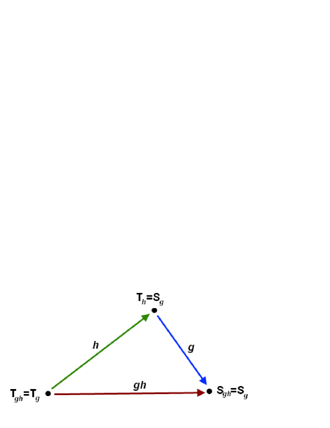
Figure 13: Composition of arrows in groupoids

Inversly, any group can be considered as a groupoid over a point. More generally, given a collection of points, then the collection of groups over those points is a groupoid.

b) arrow representation
From eqs(357-363) and the illustrating figure one also learns that each element $\mathrm{g}$ of the groupoid $\mathbb{G}$ can be represented by an arrow pointing from $T\left(g\right)$ to $S\left(g\right)$ in $\mathbb{B}$ as follows

$$T\left(g\right)\text{\ \ }\overset{g}{\longrightarrow}\text{ \ \ \ }S\left(g\right)$$ (364)

where $S$ and $T$ are the source and target maps of eq(359). In this graphic representation, to be used later on, the groupoid multiplication law corresponds then to the composition of the arrows placing the head of a given arrow $h$ to the tail of the previous one $g$ as shown on fig 13.

c) other properties
Using the arrow representation, one can read directly the basic groupoid properties; in particular the following,

$$S_{g^{-1}}$$ ,

,

(365)

and

$$\left(\lambda_{g}g\right)h$$ ,

(366)

Moreover, since for each object $x\in\mathbb{B}$, there is an identity arrow $id_{x}\in\mathbb{G}$, one can embed the set $\mathbb{B}$ of objects in the groupoid;

$$id:\mathbb{B\hookrightarrow G}$$ (367)

allowing to think about $\mathbb{B}$ as a subset of $\mathbb{G}$.

d) orbit of the groupoid
An orbit of the groupoid $\mathbb{G}$ over $\mathbb{B}$ is an equivalence class for the relation

$$x\sim_{\mathbb{G}}y$$ ,

(368)

if and only if there is a groupoid element $g\in\mathbb{G}$ such that

$$S\left(g\right)=x$$ ,

(369)

e) fibers and isotropy group
If $\mathbb{G}\rightrightarrows\mathbb{B}$ is a groupoid and $x,y\in\mathbb{B}$, then we have the following notions:
i) the source-fiber at $x$ is the set $\mathbb{G}_{x}$ of all arrows from $x$, namely

$$\mathbb{G}_{x}=\mathbb{G}\left(x,.\right)=S^{-1}\left(x\right)=\left\{g\in G\text{ }|\text{ }S\left(g\right)=x\right\}$$ (370)

ii) the target-fiber at $y$ is the set of all arrows to y, namely

$$\mathbb{G}^{y}=\mathbb{G}\left(.,y\right)=T^{-1}\left(y\right)=\left\{g\in G\text{ }|\text{ }T\left(g\right)=y\right\}$$ (371)

iii) the set of arrows from $x$ to y is

$$\mathbb{G}_{x}^{y}=\mathbb{G}\left(x,y\right)=S^{-1}\left(x\right)\cap T^{-1}\left(y\right)=\left\{g\in G\text{ }|\text{ }x\overset{g}{\rightarrow}y\right\}$$ (372)

iv) the isotropy group at $x$ is the set of self-arrows of $x$, namely

$$\mathbb{G}_{x}^{x}=\mathbb{G}\left(x,x\right)=S^{-1}\left(x\right)\cap T^{-1}\left(x\right)=\left\{g\in G\text{ }|\text{ }x\overset{g}{\rightarrow}x\right\}$$ (373)

Notice that the set $\mathbb{G}_{x}^{x}$ has a group structure; indeed the multiplication in $\mathbb{G}_{x}^{x}$ is inherited from $\mathbb{G}$; it is associative and is defined for each $g\in$ $\mathbb{G}_{x}^{x}$ since

$$S\left(x\right)=x=T\left(x\right).$$ (374)

The identity $id_{x}$ is in $\mathbb{G}_{x}^{x}$, and if $g\in$ $\mathbb{G}_{x}^{x}$, then $g^{-1}\in$ $\mathbb{G}_{x}^{x}$ since

$$S\left(g^{-1}\right)=T\left(g\right)=x=S\left(g\right)=T\left(g^{-1}\right).$$ (375)

Notice also that one might picture the sets

$$\mathbb{G}_{x}$$ , ,

(376)

as dandelions above each point in the base as in fig 14. These sets are sometimes called the star, the costar and the the vertex group respectively.

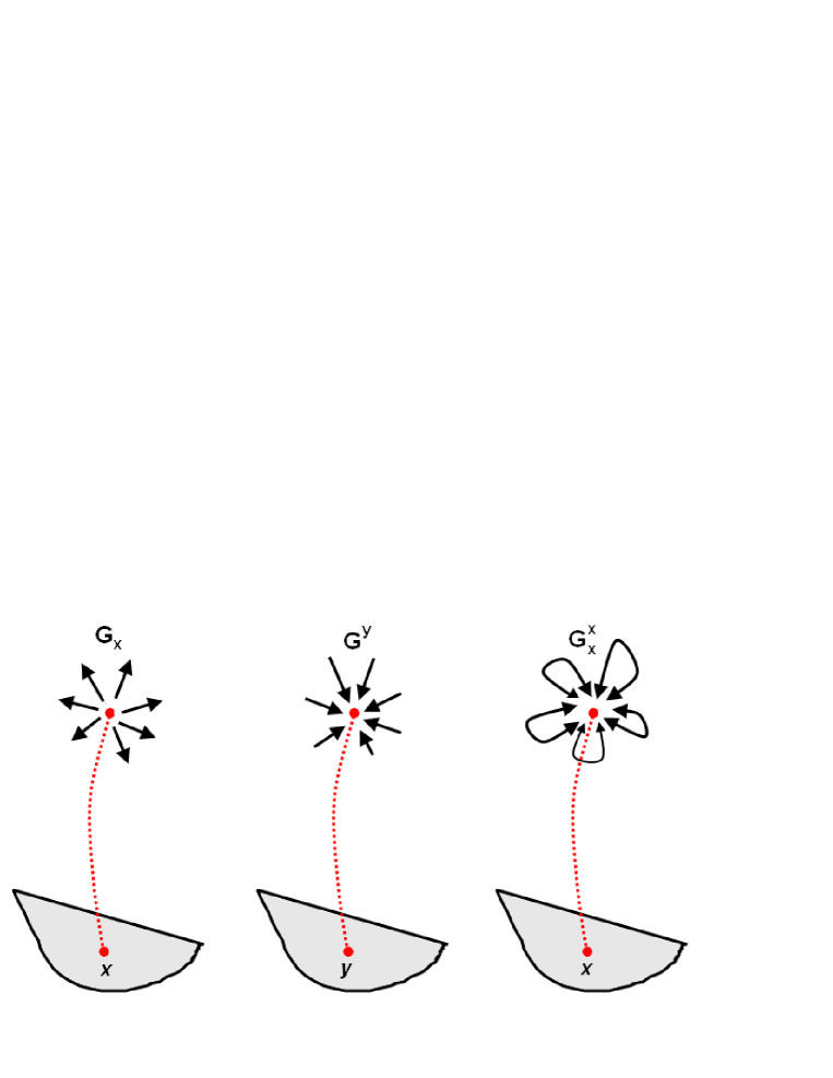
Figure 14: on left the source fiber $S^{-1}\left(x\right)$, in middle the target fiber $T^{-1}\left(y\right)$ and on right the isotropy group $S^{-1}\left(x\right)\cap T^{-1}\left(x\right)$

Along with special features given above; one can consider many other aspects of groupoids by mimicking the theory of groups; for details on some of these aspects and also for applications of groupoids in physical literature see [22] and refs therein for the important role they play in topological field theory. With these general tools at hand, we turn to the study of $\mathcal{G}_{Mut}^{G}$.

9.2 Quiver mutations

In the case of the quiver mutations considered in this paper, the base set $\mathbb{B}$ of the groupoid $\mathcal{G}_{Mut}^{G}$ is given by the chambers of the BPS quivers; in other words the objects $x$ are the quivers $\mathfrak{Q}_{n}^{G}$ with $n$ integer.

9.2.1 Mutation groupoid

In the arrow representation introduced above, the groupoid $\mathcal{G}_{Mut}^{G}$ can be pictured as the collection of the $\mathfrak{Q}_{n}^{G}$’s with the various arrows connecting them as follows:

$$\mathcal{G}_{Mut}^{G}=\left\{\mathcal{M}_{{}_{n,m}}:\text{ }\mathfrak{Q}_{n}^{G}\text{\ \ }\rightarrow\text{\ \ \ }\mathfrak{Q}_{m}^{G}\text{; \ \ }n,m\in\mathbb{Z}\text{ }\right\}$$ (377)

with $\mathcal{M}_{{}_{n,m}}$ invertible maps whose basic properties are given below. Using this arrow notation, we immediately figure out the groupoid structure of the set of mutations of BPS quivers as well as their useful properties.

$\left(a\right)$ Composition law in $\mathcal{G}_{Mut}^{G}$:
The binary operation in the set of quiver mutations $\mathcal{G}_{Mut}^{G}$ is given by the following arrow multiplication

$$\mathfrak{Q}_{n}^{G}\overset{\mathcal{M}_{{}_{n,m}}}{\longrightarrow}\mathfrak{Q}_{m}^{G}\overset{\mathcal{M}_{{}_{m,k}}}{\longrightarrow}\mathfrak{Q}_{k}^{G}\text{ \ }=\text{ \ }\mathfrak{Q}_{n}^{G}\overset{\mathcal{M}_{{}_{n,k}}}{\longrightarrow}\mathfrak{Q}_{k}^{G}$$ (378)

from which we learn that not all mutations can be composed since we should have

$$\mathcal{M}_{{}_{n,m}}\mathcal{M}_{{}_{l,k}}=\delta_{ml}\mathcal{M}_{{}_{n,k}}$$ (379)

showing that mutation pairings are defined only if $m=l$; here $\delta_{ml}$ is the usual Kronecker symbol.

$\left(b\right)$ S and T maps in $\mathcal{G}_{Mut}^{G}$
The source and target mappings $S$ and $T$ in the mutation groupoid $\mathcal{G}_{Mut}^{G}$ are given by the analogue of eqs(359); they are defined as follows

$$S\left(\mathfrak{Q}_{n}^{G}\overset{\mathcal{M}_{{}_{n,m}}}{\longrightarrow}\mathfrak{Q}_{m}^{G}\overset{\mathcal{M}_{{}_{m,k}}}{\longrightarrow}\mathfrak{Q}_{k}^{G}\right)$$

(380)

and obey eq(365).

$\left(c\right)$ Inverse in $\mathcal{G}_{Mut}^{G}$
The inverse of a generic quiver mutation of $\mathcal{G}_{Mut}^{G}$ is given by the map

$$\iota\left(\mathfrak{Q}_{n}^{G}\overset{\mathcal{M}_{{}_{n,m}}}{\longrightarrow}\mathfrak{Q}_{m}^{G}\right)$$

(381)

which, by using the definition (377), leads to

$$\mathcal{M}_{{}_{n,m}}^{-1}=\mathcal{M}_{{}_{m,n}}$$ (382)

From this relation, we also learn that in the case where $m=n$, we have

$$\mathcal{M}_{{}_{n,n}}^{-1}=\mathcal{M}_{{}_{n,n}}$$ (383)

showing that the $\mathcal{M}_{{}_{n,n}}$’s are nothing but the identities $id_{\mathfrak{Q}_{n}^{G}}$ of the mutation groupoid.

$\left(d\right)$ Left and right identities in $\mathcal{G}_{Mut}^{G}$
The left and right identities in $\mathcal{G}_{Mut}^{G}$ are as in previous relation (383); they correspond to

$$\mathfrak{Q}_{n}^{G}\overset{\mathcal{M}_{{}_{n,m}}}{\longrightarrow}\mathfrak{Q}_{m}^{G}\overset{\mathcal{M}_{{}_{m,m}}}{\longrightarrow}\mathfrak{Q}_{m}^{G}$$

(384)

which can be also written like

$$\mathfrak{Q}_{n}^{G}\overset{\mathcal{M}_{{}_{n,n}}}{\longrightarrow}\mathfrak{Q}_{n}^{G}\overset{\mathcal{M}_{{}_{n,m}}}{\longrightarrow}\mathfrak{Q}_{m}^{G}$$ (385)

From these two graphic equations, we read the left and right identities; i.e the analogue of eq(363). We also have

$$\mathcal{M}_{{}_{n,m}}\mathcal{M}_{{}_{m,m}}$$

(386)

$\left(e\right)$ Left and right multiplication in $\mathcal{G}_{Mut}^{G}$
The analogue of $\mathrm{gg}^{-1}=\mathrm{\lambda}_{g}$ is given by

$$\mathfrak{Q}_{n}^{G}\overset{\mathcal{M}_{{}_{n,m}}}{\longrightarrow}\mathfrak{Q}_{m}^{G}\overset{\mathcal{M}_{{}_{n,m}}^{-1}}{\longrightarrow}\mathfrak{Q}_{n}^{G}$$

(387)

Similarly, the analogue of $\mathrm{g}^{-1}\mathrm{g}=\mathrm{\varrho}_{g}$ is as follows

$$\mathfrak{Q}_{m}^{G}\overset{\mathcal{M}_{{}_{n,m}}^{-1}}{\longrightarrow}\mathfrak{Q}_{n}^{G}\overset{\mathcal{M}_{{}_{n,m}}}{\longrightarrow}\mathfrak{Q}_{m}^{G}$$

(388)

These relations lead respectively to

$$\mathcal{M}_{{}_{n,m}}\mathcal{M}_{{}_{n,m}}^{-1}$$

(389)

The properties (a)-(e) show that the set of BPS quiver mutations $\mathcal{G}_{Mut}^{G}$ form indeed a groupoid.

9.2.2 Examples

We end this study by giving the arrow representation of strong and weak orbits of the quiver mutations for two examples: (i) SU$\left(2\right)$ BPS theory and (ii) the SU(3) quiver theory.

SU$\left(2\right)$ case: strong and weak coupling chambers
In the arrow representation, the successive quiver mutations of the $\mathfrak{Q}_{k}^{su_{2}}$’s for both the strong and weak coupling chambers of SU$\left(2\right)$ are as depicted in fig 15.

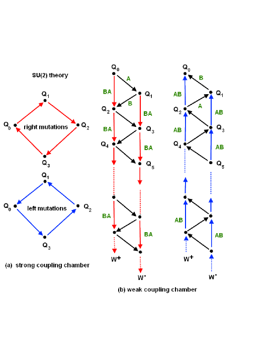
Figure 15: groupoid orbits of quiver mutations in SU$\left(2\right)$ BPS quiver theory. (a) We have represented both left and right mutations in the finite strong coupling BPS chamber from which we can learn directly the inverse of mutations, the orbit is closed and so corresponds to a periodic cycle. (b) left and right mutations of the infinite weak coupling BPS chamber. Right mutations are the inverse of left ones. $W^{\pm}$ refer to the quiver of gauge bosons corresponding to alternate singular limits of the mutations.

the strong coupling chamber is represented by a closed loop while the weak one is given by open sequences that culminate at two singular limits describing the two gauge particles $W^{\pm}$ as depicted in the figure. The divergence of the limit $k\rightarrow\infty$ is due to the alternate property of the sequences (270) namely

$$\mathcal{L}_{m}=\left(\mathcal{L}_{2k},\mathcal{L}_{2k+1}\right),\qquad\mathcal{R}_{m}=\left(\mathcal{R}_{2k},\mathcal{R}_{2k+1}\right)$$ (390)

obeying

$$\det\mathcal{L}_{2k}$$

(391)

and

$$A:$$

(392)

with $\det A=\det B=-1.$

SU$\left(3\right)$ case: strong coupling chamber
The arrow representation of the $SU\left(3\right)$ BPS quiver theory is very rich; it involves 4 basic reflections $s_{1},s_{2}$ and $t_{1},t_{2}$ whose matrix realisations are as in eq(123). Because of the property $s_{i}t_{i}=t_{i}s_{i}$, we have considered their composition

$$L_{i}=s_{i}t_{i}$$ (393)

to build the strong coupling BPS chamber whose sequence of arrows is given by fig 16.

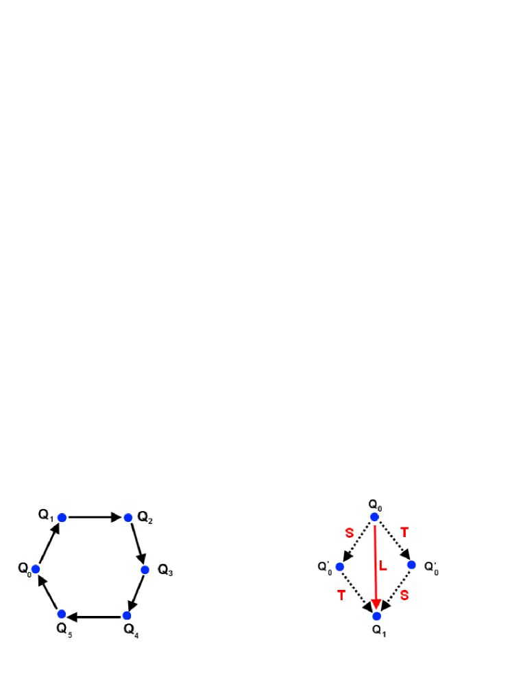
Figure 16: (a) groupoid orbit of mutations in the strong coupling chamber with isotropy group $\mathcal{G}_{strong}^{su_{3}}$. (b) arrow representation of eqs(122-128) describing the commuting reflections $s_{i}t_{i}=t_{i}s_{i}=L_{i}.$

This closure of the arrow flows extends to the strong coupling BPS chambers of all $\mathcal{N}=2$ supersymmetric QFTs with ADE gauge symmetries.

SU$\left(3\right)$ case: weak coupling chambers
In the weak coupling chamber of the SU$\left(3\right)$ theory, the sequences of arrows are open and are much more complex than the ones of the SU$\left(2\right)$ theory. These sequences involve infinite sub-chambers that culminate at 6 singular limits

$$W_{\alpha_{1}}^{\pm}$$ , ,

(394)

describing the 6 massive gauge bosons of the supersymmetric $SU\left(3\right)$ gauge model. In fig 17, we give those sequences of arrows describing mutations in BPS quiver theory that lead to (394).

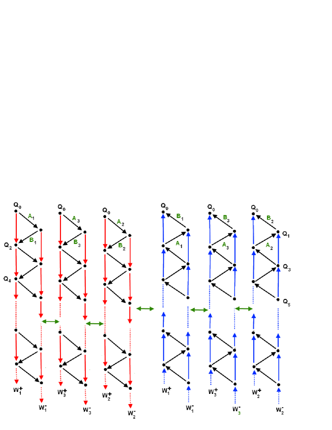
Figure 17: Weak coupling chamber of SU$\left(3\right)$ model: 6 sequences of arrows in $\mathcal{G}_{weak}^{su_{3}}$ representing left and right mutations in SU$\left(3\right)$ BPS quiver theory; each sub-chamber, made of the sequence $A_{i}B_{i}...A_{i}B_{i}$ and inverses, is isomorphic to the SU(2) chamber of fig 15. These sequences tend towards 6 singular limits corresponding to the 6 massive gauge bosons of the SU$\left(3\right)$ BPS quiver theory. Dahed cross arrows between the linear sequences are to indicate the passage between subchambers.

The alternate sequences of this figure are given by

$$\mathcal{L}_{m}^{\left(\alpha\right)}=\left(\mathcal{L}_{2k}^{\left(\alpha\right)},\mathcal{L}_{2k+1}^{\left(\alpha\right)}\right),\qquad\mathcal{R}_{m}^{\left(\alpha\right)}=\left(\mathcal{R}_{2k}^{\left(\alpha\right)},\mathcal{R}_{2k+1}^{\left(\alpha\right)}\right)$$ (395)

obeying

$$\det\mathcal{L}_{2k}^{\left(\alpha\right)}$$

(396)

with

$$A_{\alpha}:$$

(397)

and $\det A_{\alpha}=\det B_{\alpha}=-1$ and where $\alpha$ a positive root of $SU\left(3\right).$

10 Appendix II: Extension to generic $SU\left(N\right)$ models

In this appendix, we extend the analysis performed in section 4 to $\mathcal{N}=2$ supersymmetric QFTs with spontaneously broken $SU\left(N\right)$ gauge invariance down to $U^{N-1}\left(1\right)$.

10.1 Strong coupling chamber in $SU\left(N\right)$ models

We start by recalling that the number $\#_{bps}$ of BPS states in the strong coupling chamber of the $\mathcal{N}=2$ supersymmetric pure $SU\left(N\right)$ quantum field theory is given by the dimension of $SU\left(N\right)$ minus its rank $r$

$$\#_{bps}=\left(N^{2}-1\right)-N-1$$ (398)

This finite chamber includes the $\left(N-1\right)$ elementary monopoles $\mathfrak{M}_{i}$; and the $\left(N-1\right)$ elementary dyons $\mathfrak{D}_{i}$ as well as composite ones. The $\mathfrak{M}_{i}$ and $\mathfrak{D}_{i}$ particles have respective complex central charges $X_{i}$, $Y_{i}\$and EM charge vectors $b_{i},$ $c_{i}$. The latters are 2r-dimensional vectors which read in terms of the simple roots $\alpha_{i}$ of $SU\left(N\right)$ as follows

$$b_{i}=\left(\begin{array}[]{c}0\\ \alpha_{i}\end{array}\right)$$,

(399)

The strong coupling chamber contains also an equal number of anti-BPS states with negative EM charge vectors $-b_{i}$ and $-c_{i}$. So the total number of BPS and anti-BPS states is $2N\left(N-1\right)$. By using the rank $r=N-1$ of the $SU\left(N\right)$ gauge symmetry, the total number of BPS states can be put in the form

$$\#_{bps}+\#_{anti-bps}=2r\left(r+1\right)$$ (400)

In what follows, we want to show that this number can be also interpreted in terms of the order of the mutation group $\mathcal{G}_{strong}^{su_{r+1}}$ like

$$\#_{bps}+\#_{anti-bps}=r\times\left|\mathcal{G}_{strong}^{su_{r+1}}\right|$$ (401)

with

$$\left|\mathcal{G}_{strong}^{su_{r+1}}\right|=2\left(r+1\right)\equiv\mathrm{g}$$ (402)

Recall that in the cases of leading $SU\left(r+1\right)$ gauge symmetries considered in previous sections, we have obtained the results

$$SU_{2}$$

(403)

which agree with eqs(402-401). Recall also that these chambers correspond to the central charges of the elementary BPS states with arguments $\arg X_{i},$ $\arg Y_{i}$ constrained as follows

$$\arg Y_{i}$$ ,

,

(404)

and

$$\arg Y>\arg X$$ .

(405)

The derivation of the BPS states is obtained by performing quiver mutations of the quiver $\mathfrak{Q}_{0}^{su_{N}}$ made by the elementary BPS states. Extending the method we have used for $SU\left(2\right)$, $SU\left(3\right)$ and $SU\left(4\right)$ to generic N, the BPS and anti-BPS states are read from the rows of the matrix mutations $\mathcal{M}_{n}$ mapping the quiver $\mathfrak{Q}_{0}^{su_{N}}$ into $\mathfrak{Q}_{n}^{su_{N}}$ with $0<n\leq 2N$. The mutation matrices $\mathcal{M}_{n}$ are constructed below.

10.2 Building $\mathcal{G}_{strong}^{su_{N}}$

Here we build the discrete symmetry $\mathcal{G}_{strong}^{su_{N}}$ of mutation transformations interchanging the BPS quivers of the strong coupling chamber of the $\mathcal{N}=2$ supersymmetric pure $SU\left(N\right)$ quantum field theory.
To that purpose, we use special properties of the two matrix generators $L_{1}$ and $L_{2}$ of the mutations. These generators are triangular matrices of the form

$$L_{1}=\left(\begin{array}[]{cccccc}I_{r}&\cdots&0&&&\\ \vdots&\ddots&0&&{\Large S}&\\ 0&\cdots&I_{r}&&&\\ &&&-I_{r}&\cdots&0\\ &{\Large 0}&&\vdots&\ddots&\vdots\\ &&&0&\cdots&-I_{r}\end{array}\right)$$ (406)

and

$$L_{2}=\left(\begin{array}[]{cccccc}-I_{r}&\cdots&0&&&\\ \vdots&\ddots&0&&{\Large 0}&\\ 0&\cdots&-I_{r}&&&\\ &&&I_{r}&\cdots&0\\ &{\Large S}&&\vdots&\ddots&\vdots\\ &&&0&\cdots&I_{r}\end{array}\right)$$ (407)

with $I_{r}$ standing for the $r\times r$ identity matrix and the $r^{2}\times r^{2}$ matrix $S$ as follows

$$S=\left(\begin{array}[]{cccccc}0&I_{r}&0&\cdots&&0\\ I_{r}&0&I_{r}&&&0\\ 0&I_{r}&0&&&\\ \vdots&&&\ddots&&\\ 0&&&&&I_{r}\\ 0&&\cdots&&I_{r}&0\end{array}\right)$$ (408)

These are non commuting matrices, $L_{1}L_{2}\neq L_{2}L_{1}$, obeying

$$\left(L_{1}\right)^{2}=\left(L_{2}\right)^{2}=I_{id}$$ (409)

as well as identities extending eqs(76-77), (115-116) and (162-163) that can be put in the form

$$\left\langle L_{1},L_{2}|\text{ }\left(L_{i}L_{j}\right)^{m_{ij}}=I_{id}\left.\begin{array}[]{c}\\ \\ \end{array}\right.\right\rangle$$ (410)

with $m_{ij}$ the entries of the matrix

$$M=\left(\begin{array}[]{cc}1&N\\ N&1\end{array}\right)$$ (411)

Using the expression of the $L_{1}$ and $L_{2}$ matrices, one can explicitly check, after a lengthy but straightforward calculations, that the set $\mathcal{G}_{strong}^{su_{N}}$ is a non abelian symmetry with $2N$ elements. In the case $N=2K$ for instance, the group elements are given by

$$\mathcal{G}_{strong}^{su_{N}}=\left\{\begin{tabular}[]{lll}$I_{id};$&&\\ $\mathcal{M}_{2},\mathcal{M}_{4},...,\mathcal{M}_{2N-2}$&$;$&$\mathcal{M}_{1},\mathcal{M}_{3},...,\mathcal{M}_{2N-1}$\end{tabular}\right\}$$ (412)

or equivalently

$$\mathcal{G}_{strong}^{su_{N}}=\left\{\begin{tabular}[]{lll}$I_{id};$&&\\ $\mathcal{N}_{2},\mathcal{N}_{4},...,\mathcal{N}_{2N-2}$&$;$&$\mathcal{N}_{1},\mathcal{N}_{3},...,\mathcal{N}_{2N-1}$\end{tabular}\right\}$$ (413)

where we have set

$$\mathcal{M}_{2k}$$

(414)

and

$$\mathcal{M}_{2k+1}$$

(415)

We also have the identities

$$\mathcal{M}_{K}=\mathcal{N}_{K}$$ ,

(416)

and the periodic properties

$$\mathcal{M}_{0}=\mathcal{M}_{2N}$$

(417)

Notice that the $\mathcal{M}_{n}$ and $\mathcal{N}_{m}$ mutation matrices satisfy as well as

$$\mathcal{M}_{n}\mathcal{M}_{m}$$

(418)

and

$$\mathcal{M}_{n}\mathcal{N}_{m}=\left\{\begin{array}[]{ccc}\mathcal{M}_{n-m}&\text{if }&n>m\\ I_{id}&\text{if }&n=m\\ \mathcal{N}_{m-n}&\text{if }&n<m\end{array}\right.$$ (419)

From these relations, we learn that the subset $\left\{\mathcal{M}_{2n},\mathcal{N}_{2n}\right\}$ with $0\leq n\leq N$ of $\mathcal{G}_{strong}^{su_{N}}$ form a discrete abelian subsymmetry isomorphic to $\mathbb{Z}_{N}$.

11 Appendix III: Quiver mutations in $E_{6}$ model

In this appendix, we give the explicit expressions of the mutation matrices $\mathcal{M}_{n}$ relating the various BPS quivers $\mathfrak{Q}_{n}^{E_{6}}$ of the strong coupling chamber of the 4D space time $\mathcal{N}=2$ supersymmetric E₆ gauge theory spontaneously broken down to $U^{6}\left(1\right)$. From these matrices $\mathcal{M}_{n}$, one learns directly the EM charge vectors

$$b_{1}^{\left(n\right)},...,b_{6}^{\left(n\right)}$$ ,

(420)

of the BPS states and their anti-BPS partners as the rows of the $\mathcal{M}_{n}$’s. One also learns the intersection matrices by help of the formula

$$\mathcal{A}^{\left(n\right)}$$

(421)

From the results of section 5, it follows that the $\mathcal{M}_{n}$ mutations are $144\times 144$ matrices generated by $L_{1}$ and $L_{2}$ given by

$$L_{1}=\left(\begin{array}[]{cccccccccccc}{\small I}&{\small 0}&{\small 0}&{\small 0}&{\small 0}&{\small 0}&{\small 0}&{\small I}&{\small 0}&{\small 0}&{\small 0}&{\small 0}\\ {\small 0}&{\small I}&{\small 0}&{\small 0}&{\small 0}&{\small 0}&{\small I}&{\small 0}&{\small I}&{\small 0}&{\small 0}&{\small 0}\\ {\small 0}&{\small 0}&{\small I}&{\small 0}&{\small 0}&{\small 0}&{\small 0}&{\small I}&{\small 0}&{\small I}&{\small I}&{\small 0}\\ {\small 0}&{\small 0}&{\small 0}&{\small I}&{\small 0}&{\small 0}&{\small 0}&{\small 0}&{\small I}&{\small 0}&{\small 0}&{\small 0}\\ {\small 0}&{\small 0}&{\small 0}&{\small 0}&{\small I}&{\small 0}&{\small 0}&{\small 0}&{\small I}&{\small 0}&{\small 0}&{\small I}\\ {\small 0}&{\small 0}&{\small 0}&{\small 0}&{\small 0}&{\small I}&{\small 0}&{\small 0}&{\small 0}&{\small 0}&{\small I}&{\small 0}\\ {\small 0}&{\small 0}&{\small 0}&{\small 0}&{\small 0}&{\small 0}&{\small-I}&{\small 0}&{\small 0}&{\small 0}&{\small 0}&{\small 0}\\ {\small 0}&{\small 0}&{\small 0}&{\small 0}&{\small 0}&{\small 0}&{\small 0}&{\small-I}&{\small 0}&{\small 0}&{\small 0}&{\small 0}\\ {\small 0}&{\small 0}&{\small 0}&{\small 0}&{\small 0}&{\small 0}&{\small 0}&{\small 0}&{\small-I}&{\small 0}&{\small 0}&{\small 0}\\ {\small 0}&{\small 0}&{\small 0}&{\small 0}&{\small 0}&{\small 0}&{\small 0}&{\small 0}&{\small 0}&{\small-I}&{\small 0}&{\small 0}\\ {\small 0}&{\small 0}&{\small 0}&{\small 0}&{\small 0}&{\small 0}&{\small 0}&{\small 0}&{\small 0}&{\small 0}&{\small-I}&{\small 0}\\ {\small 0}&{\small 0}&{\small 0}&{\small 0}&{\small 0}&{\small 0}&{\small 0}&{\small 0}&{\small 0}&{\small 0}&{\small 0}&{\small-I}\end{array}\right)$$ (422)

and

$$L_{2} = \left(\begin{array}[]{cccccccccccc}{\small-I}&{\small 0}&{\small 0}&{\small 0}&{\small 0}&{\small 0}&{\small 0}&{\small 0}&{\small 0}&{\small 0}&{\small 0}&{\small 0}\\ {\small 0}&{\small-I}&{\small 0}&{\small 0}&{\small 0}&{\small 0}&{\small 0}&{\small 0}&{\small 0}&{\small 0}&{\small 0}&{\small 0}\\ {\small 0}&{\small 0}&{\small-I}&{\small 0}&{\small 0}&{\small 0}&{\small 0}&{\small 0}&{\small 0}&{\small 0}&{\small 0}&{\small 0}\\ {\small 0}&{\small 0}&{\small 0}&{\small-I}&{\small 0}&{\small 0}&{\small 0}&{\small 0}&{\small 0}&{\small 0}&{\small 0}&{\small 0}\\ {\small 0}&{\small 0}&{\small 0}&{\small 0}&{\small-I}&{\small 0}&{\small 0}&{\small 0}&{\small 0}&{\small 0}&{\small 0}&{\small 0}\\ {\small 0}&{\small 0}&{\small 0}&{\small 0}&{\small 0}&{\small-I}&{\small 0}&{\small 0}&{\small 0}&{\small 0}&{\small 0}&{\small 0}\\ {\small 0}&{\small I}&{\small 0}&{\small 0}&{\small 0}&{\small 0}&{\small I}&{\small 0}&{\small 0}&{\small 0}&{\small 0}&{\small 0}\\ {\small I}&{\small 0}&{\small I}&{\small 0}&{\small 0}&{\small 0}&{\small 0}&{\small I}&{\small 0}&{\small 0}&{\small 0}&{\small 0}\\ {\small 0}&{\small I}&{\small 0}&{\small I}&{\small I}&{\small 0}&{\small 0}&{\small 0}&{\small I}&{\small 0}&{\small 0}&{\small 0}\\ {\small 0}&{\small 0}&{\small I}&{\small 0}&{\small 0}&{\small 0}&{\small 0}&{\small 0}&{\small 0}&{\small I}&{\small 0}&{\small 0}\\ {\small 0}&{\small 0}&{\small I}&{\small 0}&{\small 0}&{\small I}&{\small 0}&{\small 0}&{\small 0}&{\small 0}&{\small I}&{\small 0}\\ {\small 0}&{\small 0}&{\small 0}&{\small 0}&{\small I}&{\small 0}&{\small 0}&{\small 0}&{\small 0}&{\small 0}&{\small 0}&{\small I}\end{array}\right)$$ (435)

where each entry stands for a diagonal $12\times 12$ matrix: that is $0=0_{12\times 12}$ and $I=I_{12\times 12}$. From these matrices, we can compute the set of mutations

$$\mathcal{G}_{M}^{E_{6}}=\left\{\begin{tabular}[]{lll}$\mathcal{M}_{2k}$&$=\left(L_{2}L_{1}\right)^{k}$&\\ $\mathcal{M}_{2k+1}$&$=L_{1}\mathcal{M}_{2k}$&\end{tabular};\text{ \ }0\leq k\leq 11\right\}$$ (436)

We construct below the explicit expressions of these matrices.

•  matrix $\mathcal{M}_{1}$ and quiver $\mathfrak{Q}_{1}^{E_{6}}$

  This matrix is equal to the generator $L_{1}$; then the EM charge vectors of the BPS states of the quiver $\mathfrak{Q}_{1}^{E_{6}}$ are as follows:

  $$\mathfrak{Q}_{1}^{E_{6}}:\left\{\begin{tabular}[]{lll}$b_{1}+c_{2},$&$b_{2}+c_{1}+c_{3},$&$b_{3}+c_{2}+c_{4}+c_{5},$\\ $b_{4}+c_{3},$&$b_{5}+c_{3}+c_{6},$&$b_{6}+c_{5},$\end{tabular}\right\}$$ (437)

•  the quiver $\mathfrak{Q}_{2}^{E_{6}}$

  the matrix $\mathcal{M}_{2}$ is given by $L_{2}L_{1}$ and reads explicitly as

  $$\mathcal{M}_{2}=\left(\begin{array}[]{cccccccccccc}-1&0&0&0&0&0&0&-1&0&0&0&0\\ 0&-1&0&0&0&0&-1&0&-1&0&0&0\\ 0&0&-1&0&0&0&0&-1&0&-1&-1&0\\ 0&0&0&-1&0&0&0&0&-1&0&0&0\\ 0&0&0&0&-1&0&0&0&-1&0&0&-1\\ 0&0&0&0&0&-1&0&0&0&0&-1&0\\ 0&1&0&0&0&0&0&0&1&0&0&0\\ 1&0&1&0&0&0&0&1&0&1&1&0\\ 0&1&0&1&1&0&1&0&2&0&0&1\\ 0&0&1&0&0&0&0&1&0&0&1&0\\ 0&0&1&0&0&1&0&1&0&1&1&0\\ 0&0&0&0&1&0&0&0&1&0&0&0\end{array}\right)$$ (438)

  The rows of this matrix give the EM $b_{i}^{\left(2\right)}$ and $c_{i}^{\left(2\right)}$ charge vectors of the BPS states of the quiver $\mathfrak{Q}_{2}^{E_{6}}$:

  $$\mathfrak{Q}_{2}^{E_{6}}:\left\{\begin{tabular}[]{lll}$b_{2}+c_{3},$&$b_{1}+b_{3}+c_{2}+c_{4}+c_{5},$&$b_{2}+b_{4}+b_{5}+c_{1}+2c_{3}+c_{6}$\\ $b_{5}+c_{3},$&$b_{3}+b_{6}+c_{2}+c_{4}+c_{5},$&$b_{3}+c_{2}+c_{5}$\end{tabular}\right\}$$ (439)

  This quiver has also 6 BPS states.

•  the quiver $\mathfrak{Q}_{3}^{E_{6}}$

  The mutation matrix $\mathcal{M}_{3}=L_{1}\mathcal{M}_{2}$ reads as:

  $$\mathcal{M}_{3}=\left(\begin{array}[]{cccccccccccc}0&0&1&0&0&0&0&0&0&1&1&0\\ 0&1&0&1&1&0&0&0&2&0&0&1\\ 1&0&2&0&0&1&0&2&0&1&2&0\\ 0&1&0&0&1&0&1&0&1&0&0&1\\ 0&1&0&1&1&0&1&0&2&0&0&0\\ 0&0&1&0&0&0&0&1&0&1&0&0\\ 0&-1&0&0&0&0&0&0&-1&0&0&0\\ -1&0&-1&0&0&0&0&-1&0&-1&-1&0\\ 0&-1&0&-1&-1&0&-1&0&-2&0&0&-1\\ 0&0&-1&0&0&0&0&-1&0&0&-1&0\\ 0&0&-1&0&0&-1&0&-1&0&-1&-1&0\\ 0&0&0&0&-1&0&0&0&-1&0&0&0\end{array}\right)$$ (440)

  The BPS states are as follows

  $$\mathfrak{Q}_{3}^{E_{6}}:\left\{\begin{tabular}[]{lll}$b_{3}+c_{4}+c_{5},$&$b_{2}+b_{4}+b_{5}+2c_{3}+c_{6},$&$b_{1}+2b_{3}+b_{6}+2c_{2}+c_{4}+2c_{5}$\\ $b_{3}+c_{2}+c_{4},$&$b_{2}+b_{4}+b_{5}+c_{1}+2c_{3},$&$b_{2}+b_{5}+c_{1}+c_{3}+c_{6}$\end{tabular}\right\}$$ (441)

  and there are also 6 new BPS states.

• The matrix $\mathcal{M}_{4}$

  This matrix is given by

  $$\mathcal{M}_{4}=\left(\begin{array}[]{cccccccccccc}0&0&-1&0&0&0&0&0&0&-1&-1&0\\ 0&-1&0&-1&-1&0&0&0&-2&0&0&-1\\ -1&0&-2&0&0&-1&0&-2&0&-1&-2&0\\ 0&-1&0&0&-1&0&-1&0&-1&0&0&-1\\ 0&-1&0&-1&-1&0&-1&0&-2&0&0&0\\ 0&0&-1&0&0&0&0&-1&0&-1&0&0\\ 0&0&0&1&1&0&0&0&1&0&0&1\\ 0&0&2&0&0&1&0&1&0&1&2&0\\ 0&2&0&1&2&0&1&0&3&0&0&1\\ 1&0&1&0&0&1&0&1&0&1&1&0\\ 1&0&2&0&0&0&0&2&0&1&1&0\\ 0&1&0&1&0&0&1&0&1&0&0&0\end{array}\right)$$ (442)

  from which we learn the following 6 BPS states

  $$\mathfrak{Q}_{4}^{E_{6}}:\left\{\begin{tabular}[]{ll}$b_{4}+b_{5}+c_{3}+c_{6},$&$b_{2}+b_{4}+c_{1}+c_{3},$\\ $2b_{3}+b_{6}+c_{2}+c_{4}+2c_{5},$&$b_{1}+2b_{3}+2c_{2}+c_{4}+c_{5},$\\ $2b_{2}+b_{4}+2b_{5}+c_{1}+3c_{3}+c_{6}$&$b_{1}+b_{3}+b_{6}+c_{2}+c_{4}+c_{5}$\end{tabular}\right\}$$ (443)

• the matrix $\mathcal{M}_{5}$

  We have

  $$\mathcal{M}_{5}=\left(\begin{array}[]{cccccccccccc}0&0&1&0&0&1&0&1&0&0&1&0\\ 0&1&0&1&2&0&1&0&2&0&0&1\\ 1&0&3&0&0&1&0&2&0&2&2&0\\ 0&1&0&1&1&0&0&0&2&0&0&0\\ 0&2&0&1&1&0&1&0&2&0&0&1\\ 1&0&1&0&0&0&0&1&0&0&1&0\\ 0&0&0&-1&-1&0&0&0&-1&0&0&-1\\ 0&0&-2&0&0&-1&0&-1&0&-1&-2&0\\ 0&-2&0&-1&-2&0&-1&0&-3&0&0&-1\\ -1&0&-1&0&0&-1&0&-1&0&-1&-1&0\\ -1&0&-2&0&0&0&0&-2&0&-1&-1&0\\ 0&-1&0&-1&0&0&-1&0&-1&0&0&0\end{array}\right)$$ (444)

  leading to the following 6 new BPS states

  $$\mathfrak{Q}_{5}^{E_{6}}:\left\{\begin{tabular}[]{ll}$b_{3}+b_{6}+c_{2}+c_{5}\ ,$&$b_{2}+b_{4}+2b_{5}+c_{1}+2c_{3}+c_{6}\ $\\ $b_{2}+b_{4}+b_{5}+2c_{3}\ ,$&$b_{1}+3b_{3}+b_{6}+2c_{2}+2c_{4}+2c_{5}$\\ $b_{1}+b_{3}+c_{2}+c_{5}\ ,$&$2b_{2}+b_{4}+b_{5}+c_{1}+2c_{3}+c_{6}$\end{tabular}\right\}$$ (445)

• the matrix $\mathcal{M}_{6}$

  This matrix reads as follows

  $$\mathcal{M}_{6}=\left(\begin{array}[]{cccccccccccc}0&0&-1&0&0&-1&0&-1&0&0&-1&0\\ 0&-1&0&-1&-2&0&-1&0&-2&0&0&-1\\ -1&0&-3&0&0&-1&0&-2&0&-2&-2&0\\ 0&-1&0&-1&-1&0&0&0&-2&0&0&0\\ 0&-2&0&-1&-1&0&-1&0&-2&0&0&-1\\ -1&0&-1&0&0&0&0&-1&0&0&-1&0\\ 0&1&0&0&1&0&1&0&1&0&0&0\\ 1&0&2&0&0&1&0&2&0&1&1&0\\ 0&2&0&2&2&0&1&0&3&0&0&1\\ 0&0&2&0&0&0&0&1&0&1&1&0\\ 1&0&2&0&0&1&0&1&0&1&2&0\\ 0&1&0&0&1&0&0&0&1&0&0&1\end{array}\right)$$ (446)

  leading to the BPS spectrum

  $$\mathfrak{Q}_{6}^{E_{6}}:\left\{\begin{tabular}[]{ll}$b_{2}+b_{5}+c_{1}+c_{3},$&$b_{1}+2b_{3}+b_{6}+2c_{2}+c_{5}\ \ $\\ $2b_{3}+c_{2}+c_{4}+c_{5},$&$2b_{2}+2b_{4}+2b_{5}+c_{1}+c_{4}+3c_{3}+c_{6}$\\ $b_{2}+b_{5}+c_{3}+c_{6},$&$b_{1}+2b_{3}+b_{6}+c_{2}+c_{4}+2c_{5}$\end{tabular}\right\}$$ (447)

• the matrix $\mathcal{M}_{7}$

  This matrix is given by

  $$\mathcal{M}_{7}=\left(\begin{array}[]{cccccccccccc}1&0&1&0&0&0&0&1&0&1&0&0\\ 0&2&0&1&1&0&1&0&2&0&0&0\\ 1&0&3&0&0&1&0&2&0&1&2&0\\ 0&1&0&1&1&0&1&0&1&0&0&1\\ 0&1&0&1&2&0&0&0&2&0&0&1\\ 0&0&1&0&0&1&0&0&0&1&1&0\\ 0&-1&0&0&-1&0&-1&0&-1&0&0&0\\ -1&0&-2&0&0&-1&0&-2&0&-1&-1&0\\ 0&-2&0&-2&-2&0&-1&0&-3&0&0&-1\\ 0&0&-2&0&0&0&0&-1&0&-1&-1&0\\ -1&0&-2&0&0&-1&0&-1&0&-1&-2&0\\ 0&-1&0&0&-1&0&0&0&-1&0&0&-1\end{array}\right)$$ (448)

  The corresponding BPS states are

  $$\mathfrak{Q}_{7}^{E_{6}}:\left\{\begin{tabular}[]{ll}$b_{1}+b_{3}+c_{2}+c_{4}\ ,$&$2b_{2}+b_{4}+b_{5}+c_{1}+2c_{3}\ $\\ $b_{2}+b_{4}+2b_{5}+2c_{3}+c_{6}\ ,$&$b_{1}+3b_{3}+b_{6}+2c_{2}+c_{4}+2c_{5}$\\ $b_{3}+b_{6}+c_{4}+c_{5}\ ,$&$b_{2}+b_{4}+b_{5}+c_{1}+c_{3}+c_{6}$\end{tabular}\right\}$$ (449)

• the matrix $\mathcal{M}_{8}$

  We have

  $$\mathcal{M}_{8}=\left(\begin{array}[]{cccccccccccc}-1&0&-1&0&0&0&0&-1&0&-1&0&0\\ 0&-2&0&-1&-1&0&-1&0&-2&0&0&0\\ -1&0&-3&0&0&-1&0&-2&0&-1&-2&0\\ 0&-1&0&-1&-1&0&-1&0&-1&0&0&-1\\ 0&-1&0&-1&-2&0&0&0&-2&0&0&-1\\ 0&0&-1&0&0&-1&0&0&0&-1&-1&0\\ 0&1&0&1&0&0&0&0&1&0&0&0\\ 1&0&2&0&0&0&0&1&0&1&1&0\\ 0&2&0&1&2&0&1&0&2&0&0&1\\ 1&0&1&0&0&1&0&1&0&0&1&0\\ 0&0&2&0&0&1&0&1&0&1&1&0\\ 0&0&0&1&1&0&0&0&1&0&0&0\end{array}\right)$$ (450)

  leading to

  $$\mathfrak{Q}_{8}^{E_{6}}:\left\{\begin{tabular}[]{ll}$b_{2}+b_{4}+c_{3},$&$b_{1}+2b_{3}+c_{2}+c_{4}+c_{5}$\\ $b_{1}+b_{3}+b_{6}+c_{2}+c_{5},$&$2b_{2}+b_{4}+2b_{5}+c_{1}+2c_{3}+c_{6}$\\ $b_{4}+b_{5}+c_{3},$&$2b_{3}+b_{6}+c_{2}+c_{4}+c_{5}$\end{tabular}\right\}$$ (451)

• the matrix $\mathcal{M}_{9}$

  Here we have:

  $$\mathcal{M}_{9}=\left(\begin{array}[]{cccccccccccc}{\small 0}&{\small 0}&{\small 1}&{\small 0}&{\small 0}&{\small 0}&{\small 0}&{\small 0}&{\small 0}&{\small 0}&{\small 1}&{\small 0}\\ {\small 0}&{\small 1}&{\small 0}&{\small 1}&{\small 1}&{\small 0}&{\small 0}&{\small 0}&{\small 1}&{\small 0}&{\small 0}&{\small 1}\\ {\small 1}&{\small 0}&{\small 2}&{\small 0}&{\small 0}&{\small 1}&{\small 0}&{\small 1}&{\small 0}&{\small 1}&{\small 1}&{\small 0}\\ {\small 0}&{\small 1}&{\small 0}&{\small 0}&{\small 1}&{\small 0}&{\small 0}&{\small 0}&{\small 1}&{\small 0}&{\small 0}&{\small 0}\\ {\small 0}&{\small 1}&{\small 0}&{\small 1}&{\small 1}&{\small 0}&{\small 1}&{\small 0}&{\small 1}&{\small 0}&{\small 0}&{\small 0}\\ {\small 0}&{\small 0}&{\small 1}&{\small 0}&{\small 0}&{\small 0}&{\small 0}&{\small 1}&{\small 0}&{\small 0}&{\small 0}&{\small 0}\\ {\small 0}&{\small-1}&{\small 0}&{\small-1}&{\small 0}&{\small 0}&{\small 0}&{\small 0}&{\small-1}&{\small 0}&{\small 0}&{\small 0}\\ {\small-1}&{\small 0}&{\small-2}&{\small 0}&{\small 0}&{\small 0}&{\small 0}&{\small-1}&{\small 0}&{\small-1}&{\small-1}&{\small 0}\\ {\small 0}&{\small-2}&{\small 0}&{\small-1}&{\small-2}&{\small 0}&{\small-1}&{\small 0}&{\small-2}&{\small 0}&{\small 0}&{\small-1}\\ {\small-1}&{\small 0}&{\small-1}&{\small 0}&{\small 0}&{\small-1}&{\small 0}&{\small-1}&{\small 0}&{\small 0}&{\small-1}&{\small 0}\\ {\small 0}&{\small 0}&{\small-2}&{\small 0}&{\small 0}&{\small-1}&{\small 0}&{\small-1}&{\small 0}&{\small-1}&{\small-1}&{\small 0}\\ {\small 0}&{\small 0}&{\small 0}&{\small-1}&{\small-1}&{\small 0}&{\small 0}&{\small 0}&{\small-1}&{\small 0}&{\small 0}&{\small 0}\end{array}\right)$$ (452)

  giving the BPS spectrum

  $$\mathfrak{Q}_{9}^{E_{6}}:\left\{\begin{tabular}[]{ll}$b_{3}+c_{5},$&$b_{2}+b_{4}+b_{5}+c_{3}+c_{6}\ $\\ $b_{2}+b_{5}+c_{3},$&$b_{1}+2b_{3}+b_{6}+c_{2}+c_{4}+c_{5}$\\ $b_{3}+c_{2},$&$b_{2}+b_{4}+b_{5}+c_{1}+c_{3}$\end{tabular}\right\}$$ (453)

• the matrix $\mathcal{M}_{10}$

  This matrix is given by

  $$\mathcal{M}_{10}=\left(\begin{array}[]{cccccccccccc}{\small 0}&{\small 0}&{\small-1}&{\small 0}&{\small 0}&{\small 0}&{\small 0}&{\small 0}&{\small 0}&{\small 0}&{\small-1}&{\small 0}\\ {\small 0}&{\small-1}&{\small 0}&{\small-1}&{\small-1}&{\small 0}&{\small 0}&{\small 0}&{\small-1}&{\small 0}&{\small 0}&{\small-1}\\ {\small-1}&{\small 0}&{\small-2}&{\small 0}&{\small 0}&{\small-1}&{\small 0}&{\small-1}&{\small 0}&{\small-1}&{\small-1}&{\small 0}\\ {\small 0}&{\small-1}&{\small 0}&{\small 0}&{\small-1}&{\small 0}&{\small 0}&{\small 0}&{\small-1}&{\small 0}&{\small 0}&{\small 0}\\ {\small 0}&{\small-1}&{\small 0}&{\small-1}&{\small-1}&{\small 0}&{\small-1}&{\small 0}&{\small-1}&{\small 0}&{\small 0}&{\small 0}\\ {\small 0}&{\small 0}&{\small-1}&{\small 0}&{\small 0}&{\small 0}&{\small 0}&{\small-1}&{\small 0}&{\small 0}&{\small 0}&{\small 0}\\ {\small 0}&{\small 0}&{\small 0}&{\small 0}&{\small 1}&{\small 0}&{\small 0}&{\small 0}&{\small 0}&{\small 0}&{\small 0}&{\small 1}\\ {\small 0}&{\small 0}&{\small 1}&{\small 0}&{\small 0}&{\small 1}&{\small 0}&{\small 0}&{\small 0}&{\small 0}&{\small 1}&{\small 0}\\ {\small 0}&{\small 1}&{\small 0}&{\small 1}&{\small 1}&{\small 0}&{\small 0}&{\small 0}&{\small 1}&{\small 0}&{\small 0}&{\small 0}\\ {\small 0}&{\small 0}&{\small 1}&{\small 0}&{\small 0}&{\small 0}&{\small 0}&{\small 0}&{\small 0}&{\small 1}&{\small 0}&{\small 0}\\ {\small 1}&{\small 0}&{\small 1}&{\small 0}&{\small 0}&{\small 0}&{\small 0}&{\small 1}&{\small 0}&{\small 0}&{\small 0}&{\small 0}\\ {\small 0}&{\small 1}&{\small 0}&{\small 0}&{\small 0}&{\small 0}&{\small 1}&{\small 0}&{\small 0}&{\small 0}&{\small 0}&{\small 0}\end{array}\right)$$ (454)

  The 6 new BPS states are as follows

  $$\mathfrak{Q}_{10}^{E_{6}}:\left\{\begin{tabular}[]{ll}$b_{5}+c_{6},$&$b_{3}+b_{6}+c_{5}\ $\\ $b_{3}+c_{4},$&$b_{2}+b_{4}+b_{5}+c_{3}$\\ $b_{2}+c_{1},$&$b_{1}+b_{3}+c_{2}$\end{tabular}\right\}$$ (455)

• the matrix $\mathcal{M}_{11}$

  We have

  $$\mathcal{M}_{11}=\left(\begin{array}[]{cccccccccccc}{\small 0}&{\small 0}&{\small 0}&{\small 0}&{\small 0}&{\small 1}&{\small 0}&{\small 0}&{\small 0}&{\small 0}&{\small 0}&{\small 0}\\ {\small 0}&{\small 0}&{\small 0}&{\small 0}&{\small 1}&{\small 0}&{\small 0}&{\small 0}&{\small 0}&{\small 0}&{\small 0}&{\small 0}\\ {\small 0}&{\small 0}&{\small 1}&{\small 0}&{\small 0}&{\small 0}&{\small 0}&{\small 0}&{\small 0}&{\small 0}&{\small 0}&{\small 0}\\ {\small 0}&{\small 0}&{\small 0}&{\small 1}&{\small 0}&{\small 0}&{\small 0}&{\small 0}&{\small 0}&{\small 0}&{\small 0}&{\small 0}\\ {\small 0}&{\small 1}&{\small 0}&{\small 0}&{\small 0}&{\small 0}&{\small 0}&{\small 0}&{\small 0}&{\small 0}&{\small 0}&{\small 0}\\ {\small 1}&{\small 0}&{\small 0}&{\small 0}&{\small 0}&{\small 0}&{\small 0}&{\small 0}&{\small 0}&{\small 0}&{\small 0}&{\small 0}\\ {\small 0}&{\small 0}&{\small 0}&{\small 0}&{\small-1}&{\small 0}&{\small 0}&{\small 0}&{\small 0}&{\small 0}&{\small 0}&{\small-1}\\ {\small 0}&{\small 0}&{\small-1}&{\small 0}&{\small 0}&{\small-1}&{\small 0}&{\small 0}&{\small 0}&{\small 0}&{\small-1}&{\small 0}\\ {\small 0}&{\small-1}&{\small 0}&{\small-1}&{\small-1}&{\small 0}&{\small 0}&{\small 0}&{\small-1}&{\small 0}&{\small 0}&{\small 0}\\ {\small 0}&{\small 0}&{\small-1}&{\small 0}&{\small 0}&{\small 0}&{\small 0}&{\small 0}&{\small 0}&{\small-1}&{\small 0}&{\small 0}\\ {\small-1}&{\small 0}&{\small-1}&{\small 0}&{\small 0}&{\small 0}&{\small 0}&{\small-1}&{\small 0}&{\small 0}&{\small 0}&{\small 0}\\ {\small 0}&{\small-1}&{\small 0}&{\small 0}&{\small 0}&{\small 0}&{\small-1}&{\small 0}&{\small 0}&{\small 0}&{\small 0}&{\small 0}\end{array}\right)$$ (456)

  giving

  $$\mathfrak{Q}_{11}^{E_{6}}:\left\{\begin{tabular}[]{ll}$b_{6}\ ,$&$b_{4}\ $\\ $b_{5}\ ,$&$b_{2}\ $\\ $b_{3}\ ,$&$b_{1}\ $\end{tabular}\right\}$$ (457)

  which are not new BPS states as these are precisely the elementary BPS states that appear in the quiver $\mathfrak{Q}_{0}$ given by fig 10.

• the matrix $\mathcal{M}_{12}$

  This matrix reads as follows:

  $$\mathcal{M}_{12}=\left(\begin{array}[]{cccccccccccc}{\small 0}&{\small 0}&{\small 0}&{\small 0}&{\small 0}&{\small-1}&{\small 0}&{\small 0}&{\small 0}&{\small 0}&{\small 0}&{\small 0}\\ {\small 0}&{\small 0}&{\small 0}&{\small 0}&{\small-1}&{\small 0}&{\small 0}&{\small 0}&{\small 0}&{\small 0}&{\small 0}&{\small 0}\\ {\small 0}&{\small 0}&{\small-1}&{\small 0}&{\small 0}&{\small 0}&{\small 0}&{\small 0}&{\small 0}&{\small 0}&{\small 0}&{\small 0}\\ {\small 0}&{\small 0}&{\small 0}&{\small-1}&{\small 0}&{\small 0}&{\small 0}&{\small 0}&{\small 0}&{\small 0}&{\small 0}&{\small 0}\\ {\small 0}&{\small-1}&{\small 0}&{\small 0}&{\small 0}&{\small 0}&{\small 0}&{\small 0}&{\small 0}&{\small 0}&{\small 0}&{\small 0}\\ {\small-1}&{\small 0}&{\small 0}&{\small 0}&{\small 0}&{\small 0}&{\small 0}&{\small 0}&{\small 0}&{\small 0}&{\small 0}&{\small 0}\\ {\small 0}&{\small 0}&{\small 0}&{\small 0}&{\small 0}&{\small 0}&{\small 0}&{\small 0}&{\small 0}&{\small 0}&{\small 0}&{\small-1}\\ {\small 0}&{\small 0}&{\small 0}&{\small 0}&{\small 0}&{\small 0}&{\small 0}&{\small 0}&{\small 0}&{\small 0}&{\small-1}&{\small 0}\\ {\small 0}&{\small 0}&{\small 0}&{\small 0}&{\small 0}&{\small 0}&{\small 0}&{\small 0}&{\small-1}&{\small 0}&{\small 0}&{\small 0}\\ {\small 0}&{\small 0}&{\small 0}&{\small 0}&{\small 0}&{\small 0}&{\small 0}&{\small 0}&{\small 0}&{\small-1}&{\small 0}&{\small 0}\\ {\small 0}&{\small 0}&{\small 0}&{\small 0}&{\small 0}&{\small 0}&{\small 0}&{\small-1}&{\small 0}&{\small 0}&{\small 0}&{\small 0}\\ {\small 0}&{\small 0}&{\small 0}&{\small 0}&{\small 0}&{\small 0}&{\small-1}&{\small 0}&{\small 0}&{\small 0}&{\small 0}&{\small 0}\end{array}\right)$$ (458)

  Notice that the entries of this matrix are either zero or negative definite integers. The corresponding quiver $\mathfrak{Q}_{12}^{E_{6}}$ involves only anti-BPS states; and so should be viewed as the CPT conjugate of $\mathfrak{Q}_{0}^{E_{6}}$. Notice also the natural identity

  $$\left(\mathcal{M}_{12}\right)^{2}=I_{id}$$

12 Appendix IV: Coxeter groups and Coxeter graphs

In this appendix, we collect some useful tools on the building of the Coxeter groups and their basic properties. We also give the corresponding graphs and relation with the Dynkin diagrams of simple Lie algebras.

12.1 Coxeter groups

A way to introduce a generic Coxeter group is by considering the two following things: (1) a system on $n$ involutions $\left\{s_{1},...,s_{n}\right\}$ satisfying $s_{i}^{2}=1$ $\forall i$; which has to be thought of as the group generators of the group. (2) a symmetric $n\times n$ matrix $M$, known as the Coxeter matrix, with integer entries $\left(m_{ij}\right)$ constrained as

$$m_{ii}=1,\qquad m_{ij}\geq 2\text{ \ for \ }i\neq j.$$ (459)

The Coxeter group associated with the $s_{i}$’s and the matrix $M$ is generally denoted as $W\left(M\right)$ and called the Coxeter group of type $M$. This set is defined as:

$$W\left(M\right)=\left\langle\left.\begin{array}[]{cc}s_{i}^{2}&=1\\ \left(s_{i}s_{j}\right)^{m_{ij}}&=1\end{array}\right.;\text{ \ }m_{ij}\geq 2\right\rangle$$ (460)

Clearly according to the values of $m_{ij}$, the Coxeter groups $W\left(M\right)$ may be finite or infinite discrete  groups.
Coxeter groups have several remarkable properties; one of them is that giving the link between $M=\left(m_{ij}\right)$ and the usual Cartan matrix $K_{ij}$ of simple Lie algebras namely

$$K_{ij}=-2\cos\frac{\pi}{m_{ij}}$$ (461)

Besides the crucial role that play in approaching Lie algebras; this identification is also important for classifying the Coxeter groups $W\left(M\right)$ by using the determinant of the Cartan matrix $K_{ij}$. We have [36, 37]:

• finite $W\left(M\right)$ if $\det K>0$,

• affine $W\left(M\right)$ if $\det K=0$,

• hyperbolic $W\left(M\right)$ for $\det K<0$.

Notice also that Coxeter groups are deeply connected with reflection groups; including the Weyl group of simple Lie algebras, and which can be thought of as a linear representation of $W\left(M\right)$. Their group generators given by invertible $n\times n$ matrices; and so form a a subgroup of $GL\left(n,R\right)$. To illustrate these kinds of discrete groups, we give below three examples respectively concerning: the cyclic group of order 2, the dihedral groups $Dih_{2m}$ with $m>2$; and the groups $A_{n}$ associated with the $SU\left(n+1\right)$ gauge symmetries.

Example 1: cyclic group of order 2
This is the simplest Coxeter group with one generator $s$ and a Coxeter matrix $M=\left(1\right)$. Substituting, we get:

$$W\left(M\right)=\left\langle s|\text{ }s^{2}=1\right\rangle$$ (462)

which is the cyclic group $\mathbb{Z}_{2}$ of order 2. The elements of this group are $\pm I_{id}$.

Example 2: dihedral group $Dih_{2m}$
In this case, we have two group generators, which we denote as $s$ and $t$, and a Coxeter matrix M, denoted as $I_{2}\left(m\right)$, reads as follows,

$$I_{2}\left(m\right)=\left(\begin{array}[]{cc}1&m\\ m&1\end{array}\right),\qquad m\geq 2$$ (463)

This group is precisely the dihedral group $Dih_{2m}$ given by,

$$Dih_{2m}=\left\langle\left.\begin{array}[]{c}\\ \\ \end{array}\right.s,t|\text{ }s^{2}=t^{2}=1;\text{ }\left(st\right)^{m}=1,\text{ }m\geq 2\right\rangle$$ (464)

Notice that depending on the choice of the integer $m$, we have different groups. For the particular case $m=2$, the condition $\left(st\right)^{m}=\left(st\right)^{2}=1$ leads as well to

$$stst=1$$ (465)

This condition combined with $s^{2}=t^{2}=1$ leads to

$$st=s\left(stst\right)t=ts$$ (466)

showing that the group $Dih_{4}$ is abelian.
In the case $m\geq 3$, the corresponding group is non abelian; this property can be obtained by using the involutions, we have $\left(st\right)^{2}\neq 1$ which is also equal to $\left(st\right)^{-1}$. The term $\left(st\right)^{2}$ can put as the group commutator $sts^{-1}t^{-1}$ showing that $st\neq ts$.

Example 3: groups $A_{n}$
We illustrate the construction of these groups on the cases A₃ and A₄ respectively associated with the $SU\left(4\right)$ and SU$\left(5\right)$ gauge symmetries. The same thing is valid for the general case. In the case of A₃, we have three generators s, t, u  and a Coxeter matrix M as

$$M=\left(\begin{array}[]{ccc}1&3&2\\ 3&1&3\\ 2&3&1\end{array}\right)$$ (467)

from which we read the group structure

$$A_{3}=\left\langle s,t,u\text{ \ }|\text{ }\left\{\begin{array}[]{ccccc}s^{2}=1&,&t^{2}=1&,&u^{2}=1\\ \left(st\right)^{3}=1&,&\left(su\right)^{2}=1&,&\left(tu\right)^{3}=1\end{array}\right.\right\rangle$$ (468)

In the case of $SU\left(5\right)$, the Coxeter matrix is given by

$$M=\left(\begin{array}[]{cccc}1&3&2&2\\ 3&1&3&2\\ 2&3&1&3\\ 2&2&3&1\end{array}\right)$$ (469)

12.2 Coxeter diagrams

To the symmetric $n\times n$ Coxeter matrix $M=\left(m_{ij}\right)$, one associates a graph $\Gamma\left(M\right)$ having n vertices in one to one with the generators of the group $W\left(M\right)$. Two nodes $i$ and $j$ of the graph are joined by an edge labeled $m_{ij}$ if $m_{ij}>2$.
For $m_{ij}=3$ the label 3 of the edge $\left\{i,j\right\}$ is often omitted; and for $m_{ij}=4$, one often draws a double bond instead of the label $4$ at the edge $\left\{i,j\right\}$.
The data stored in the Coxeter matrix $M$ can be reconstructed from the Coxeter diagram, and so the Coxeter diagram and the Coxeter matrix can be identified.
We end this appendix by the two following things: First, the ADE Dynkin graphs of fig 3 are particular Coxeter diagrams; the relation between the two diagrams is given by eq(461); see also fig 18.

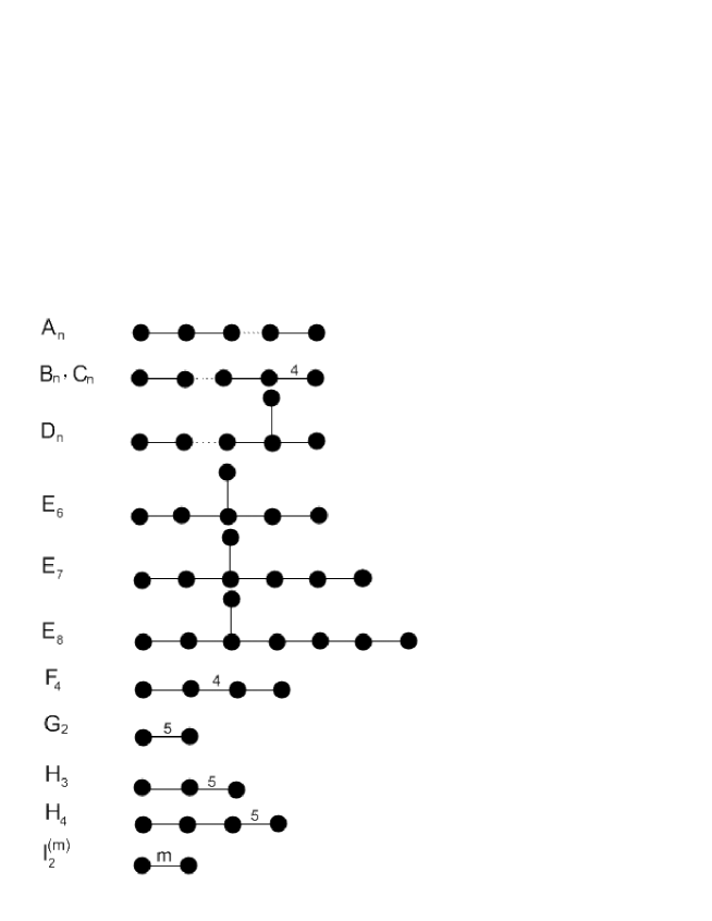
Figure 18: Diagrams of irreducible finite Coxeter systems; the diagrams $G_{2}$ and $I_{2}^{\left(6\right)}$ are the same. The diagrams $H_{2}$ and $B_{2}$ might be defined as $I_{2}^{\left(5\right)}$ and $I_{2}^{\left(4\right)}$ respectively. The diagram $A_{2}$ coincides with $I_{2}^{\left(3\right)}.$

Second, the Coxeter number $h$ is the order of a Coxeter element of an irreducible Coxeter group. A Coxeter element of $W\left(M\right)$ is given by the product of all simple reflections. The number $h$ and its dual $\tilde{h}$ of finite dimensional Lie algebras are collected in the following table

graphs      $$\ h$$

(470)

References

• [1] Murad Alim, Sergio Cecotti, Clay Cordova, Sam Espahbodi, Ashwin Rastogi, Cumrun Vafa, BPS Quivers and Spectra of Complete $\mathcal{N}$=2 Quantum Field Theories, arXiv:1109.4941,
• [2] Murad Alim, Sergio Cecotti, Clay Cordova, Sam Espahbodi, Ashwin Rastogi, Cumrun Vafa, $\mathcal{N}$=2 Quantum Field Theories and Their BPS Quivers, arXiv:1112.3984,
• [3] N. Seiberg, Electric-magnetic duality in supersymmetric non abelian gauge theories, Nucl.Phys. B435 (1995) 129146, arXiv:hep-th/9411149 [hep-th].
• [4] N. Seiberg and E. Witten, Electric-magnetic duality, monopole condensation, and confinement in N=2 supersymmetric Yang-Mills theory, Nucl.Phys. B426 (1994) 1952, arXiv:hep-th/9407087 [hep-th].
• [5] N. Seiberg and E. Witten, Monopoles, duality and chiral symmetry breaking in N=2 supersymmetric QCD, Nucl.Phys. B431 (1994) 484550, arXiv:hep-th/9408099 [hep-th].
• [6] A. Klemm, W. Lerche, S. Yankielowicz, and S. Theisen. Simple singularities and $\mathcal{N}=2$ supersymmetric Yang-Mills theory. Phys. Lett., B344:169–175, 1995, hep-th/9411048
• [7] Philip C. Argyres and Alon E. Faraggi. The vacuum structure and spectrum of $\mathcal{N}=2$ supersymmetric su(n) gauge theory. Phys. Rev. Lett., 74:3931–3934, 1995, hep-th/9411057,
• [8] A. Klemm, W. Lerche, S. Yankielowicz, and S. Theisen. On the monodromies of $\mathcal{N}=2$ supersymmetric Yang-Mills theory. 1994, hep-th/9412158,
• [9] Michael R. Douglas and Stephen H. Shenker. Dynamics of su(n) supersymmetric gauge theory. Nucl. Phys., B447:271–296, 1995, hep-th/9503163.
• [10] D. Gaiotto, G. W. Moore, and A. Neitzke, Wall-crossing, Hitchin Systems, and the WKB Approximation, arXiv:0907.3987 [hep-th].
• [11] Adel Bilal, Duality in $\mathcal{N}=2$ SUSY Gauge Theories: low-energy effective action and BPS spectra, arXiv:hep-th/0106246
• [12] F. Ferrari and A. Bilal, The Strong coupling spectrum of the Seiberg-Witten theory, Nucl.Phys. B469 (1996) 387402, arXiv:hep-th/9602082 [hep-th].
• [13] A. Bilal and F. Ferrari, Curves of marginal stability, and weak and strong coupling BPS spectra in $\mathcal{N}=2$ supersymmetric QCD,” Nucl.Phys. B480 (1996) 589-622, arXiv:hep-th/9605101 [hep-th].
• [14] Sergio Cecotti, Clay Cordova, Cumrun Vafa, Braids, Walls, and Mirrors, arXiv:1110.2115
• [15] S. Cecotti and C. Vafa, Classi cation of complete $\mathcal{N}=2$ supersymmetric theories in 4 dimensions, arXiv:1103.5832 [hep-th],
• [16] Sergio Cecotti, Clay Cordova, Jonathan J. Heckman, Cumrun Vafa, T-Branes and Monodromy, JHEP 1107:030,2011,
• [17] D. Gaiotto, G. W. Moore, and A. Neitzke, Four-dimensional wall-crossing via three-dimensional eld theory, Commun.Math.Phys. 299 (2010) 163-224, arXiv:0807.4723 [hep-th],
• [18] D. Gaiotto, G. W. Moore, and A. Neitzke, Framed BPS States, arXiv:1006.0146 [hep-th],
• [19] T. Dimofte, S. Gukov, and Y. Soibelman, Quantum Wall Crossing in $\mathcal{N}=2$ Gauge Theories, Lett.Math.Phys. 95 (2011) 1{25, arXiv:0912.1346 [hep-th].
• [20] Michael Yu. Kuchiev. Supersymmetric $\mathcal{N}=2$ gauge theory with arbitrary gauge group. Nucl.Phys., B838:331–357, 2010, 0907.2010.
• [21] Michael Yu. Kuchiev, Charges of dyons in $\mathcal{N}=2$ supersymmetric gauge theory, Nucl.Phys.B803:113-134,2008, arXiv:0805.1461,
• [22] S. Cecotti, A. Neitzke, and C. Vafa, R-Twisting and 4d/2d Correspondences, arXiv:1006.3435 [hep-th],
• [23] E.H Saidi, Weak Coupling Chambers in $\mathcal{N}=2$ BPS Quiver Theory, Nuclear Physics B 864 [FS] (2012) 190–202, LPHE preprint (2012),
• [24] W. Brandt, Über eine Verallgemeinerung des Gruppenbegriffes, Math. Ann. 96 (1926), 360-366,
• [25] R. Brown, From groups to groupoids: A brief survey, Bull. London Math. Soc. 19 (1987), 113–134,
• [26] C. Ehresmann, Oeuvres complètes et commentées, (A. C. Ehresmann, ed.) Suppl. Cahiers Top.Géom. Diff., Amiens, 1980–1984.
• [27] Francesco Bonechi, Maxim Zabzine, Lie algebroids, Lie groupoids and TFT, J.Geom.Phys.57:731-744,2007, arXiv:math/0512245,
• [28] F. Bonechi, N. Ciccoli, N. Staffolani, M. Tarlini, The quantization of the symplectic groupoid of the standard Podles sphere, arXiv:1004.3163,
• [29] J.H. Lu and A.Weinstein, Groupoides symplectiques doubles de groupes de Lie-Poisson, Comptes Rendus de Seances, Academie de Sciences (Paris), Serie I. Mathematique, 309 (1989), 951-954.
• [30] K. C. H. Mackenzie, General theory of Lie groupoids and Lie algebroids, Cambridge University Press, Cambridge, 2005. xxxviii+501 pp.
• [31] A. Belhaj, E.H Saidi, Toric Geometry, Enhanced non Simply laced Gauge Symmetries in Superstrings and F-theory Compactifications, arXiv:hep-th/0012131,
• [32] Loriano Bonora, Raffaele Savelli, Non-simply-laced Lie algebras via F theory strings, JHEP 1011:025,2010, arXiv:1007.4668,
• [33] U. H. Danielsson, B. Sundborg, The moduli space and monodromies of N=2 supersymmetric so$\left(2r+1\right)$ Yang-Mills theory, Phys. Lett. B358 (1995) 273–280, arXiv:hep-th/9504102,
• [34] M. R. Abolhasani, M. Alishahiha, A. M. Ghezelbash, The moduli space and monodromies of the N=2 supersymmetric Yang-Mills theory with any Lie gauge groups, Nucl. Phys. B480 (1996) 279–295. arXiv:hep-th/9606043.
• [35] K. Landsteiner, J. M. Pierre, S. B. Giddings, On the moduli space of N=2 supersymmetric G2 gauge theory, Phys. Rev. D55 (1997) 2367–2372, arXiv:hep-th/9609059.
• [36] M. Ait Ben Haddou, A. Belhaj, E.H. Saidi, Nucl.Phys. B674 (2003) 593-614, arXiv:hep-th/0307244,
• [37] R. Ahl Laamara, M. Ait Ben Haddou, A Belhaj, L.B Drissi, E.H Saidi, Nucl.Phys. B702 (2004) 163-188, arXiv:hep-th/0405222,
Malika Ait Benhaddou, El Hassan Saidi, Physics Letters B575 (2003)100-110, arXiv:hep-th/0307103,
• [38] Alan Weinstein, Groupoids: unifying internal and external symmetry, Notices Amer. Math. Soc. 43 (1996), 744–752, arXiv:math/9602220,
• [39] Ieke Moerdijk, Orbifolds as Groupoids: an Introduction, arXiv:math/0203100,
S. MacLane, Categories for the Working Mathematician, SpringerVerlag, 1971.