Shape- and topology-dependent heat capacity of few-particle systems

Abstract

Thermal properties of few-fermion ($n<5$) systems are investigated. The dependence of the heat capacity on the topology and shape of the cavity containing the particles is analyzed. It is found that the maximum of the heat capacity, occuring at low $T$, discussed recently by Toutounji for a system with $n=1$ fermions, is even more visible for $n=2$, but fades away for $n=3$ and $4$. For large $T$, the classical behavior is obtained; however, when $T\rightarrow 0$, the heat capacity tends to zero exponentially, not linearly, as in macroscopic and even mesoscopic systems. The physical relevance of these results is discussed.

1 Introduction

Recent progress in nanophysics has stimulated the interest in studying particles confined to small volumes or in atypical geometries. If we are focused on the theoretical study of thermal properties of such systems, the contribution of translational degrees of freedom of the constituents to the partition function of the system might be evaluated taking into account the discrete character of the particle wave vectors.

To be more specific, let us mention that, for non-interacting many-particle systems, the translational part of the canonical partition function is evaluated in the thermodynamic limit, as an integral over the particle momenta; however, for few-particle systems, confined to small cavities, this quantity should be obtained as a discrete sum over the quantized values of the particle wave vectors. Recently, Toutounji [1] analyzed the thermal properties of an electron confined to  a segment, using the canonical ensemble, showing that the heat capacity of this one-particle system has a bump, at ”low” temperatures, i.e. when $k_{B}T$ is much lower than the ground state energy (the quotation marks intend to remind that, in this context, the room temperature is a ”low” temperature). Of course, as $T$ increases, the heat capacity reaches asymptotically the value $k_{B}/2$. The existence of this bump is smeared out in the thermodynamic limit. We can presume that other interesting effects, specific to few-particle systems, are detectable only taking into account the discrete character of physical parameters describing such systems. A critical discussion of Toutounji’s approach, from the perspective of the foundations of statistical mechanics, has been done by Lungu [2].

It is legitimate to wonder about the physical relevance of few–particle thermodynamics. There are several aspects to be discussed: (1) is it meaningful to speak about thermal properties of few particle systems, knowing that thermal physics works essentially with large systems? (2) if the response is positive, is the canonical ensemble appropriate for such investigations? (3) there is a real physical interest for the study of thermal behavior of few-particle systems?

If the particles are confined to a cavity in thermal equilibrium with a thermostat, they reach thermal equilibrium not through mutual interaction (the typical case studied by statistical mechanics), but mainly through interaction with cavity’s walls and with thermal radiation. In fact, the calculation of the one-particle partition sum for particles in simple external potentials is a common exercise in several books of quantum mechanics or quantum statistical physics (see for instance [3], [4]). However, as the thermodynamic relations are obtained, in general, in the thermodynamic limit, the significance of results referring to few particle systems, must be considered with caution [2].

Concerning the second issue, let us recall - invoking again the detailed analyses done by Lungu [2] - that the grand-canonical system is the most appropriate for statistical mechanics calculations, because the quantum statistical properties of particles are automatically taken into account. However, we can use the canonical ensemble, if we correctly define the quantum states and their degeneracies. This can be done quite easily for few particles, but becomes a quite cumbersome exercise if the number of particles increases. It is important to stress the fact that the canonical partition function of a quantum few-particle system does not factorize, in terms of one-particle partition functions. This is why the results obtained for a one-particle system have no relevance for several-particle systems.

Finally, the study of few-particle systems is not an academic exercise, as such systems are available and have very interesting properties, the most popular being the electrons in quantum dots and atoms in Bose-Einstein condensates (BEC), see for instance [5], [6]). Investigations in quantum field theory provide another reason for calculating the one-particle partition function, for instance of a particle in an anharmonic potential [7]. Let us also mention that the last paper of Feynman presents a method for approximating the quantum partition function with a classical one [8].

The starting point of the investigations presented in this paper is the attempt to reconcile the heat capacity behavior obtained by Toutounji for a one-electron system - which shows an maximum at low temperature, as already mentioned - and the well-known aspect of this quantity, for a macroscopic body, which starts from zero at $T=0$, increases smoothly while $T$ increases, reaching an horizontal asymptote for $T\rightarrow\infty$. In fact, the same smooth behavior occurs for mesoscopic systems with as few as $n=14$ particles, as shown by Lungu [2]. So, we are trying to bridge the results obtained by Toutounji, for a system with $n=1$ particles, with the results obtained by Lungu, for a system with $n=14$ particles. We evaluated approximately the canonic partition function, for a system of 2, 3 and 4 free fermions, taking into account the exclusion principle - so considering that the particles are indeed fermions - and found out that the low-$T$ maximum occurring for an one-electron system decreases for systems with 3 and 4 particles (even if it is enhanced for a 2-particle system), and the aspect of the heat capacity plot becomes smoother. So, our results bridge the one-particle behavior of the heat capacity, obtained by Toutounji, with the mesoscopic behavior, obtained by Lungu, which in fact does not differ qualitatively from the macroscopic behavior.

However, there is another ”anomaly” which is noticed in the heat capacity of few-body systems. If, for macroscopic systems (see for instance [9], Ch.6), and even for mesoscopic ones [2], the heat capacity decreases like $T$ when $T\rightarrow 0$, in the cases discussed here (1, 2, 3 and 4 particles) it behaves like $e^{-1/\tau}/\tau^{2}$, where $\tau$ is a scaled temperature. Such a behavior is compatible with Toutounji’s results, even if this issue is not explicitly discussed in his paper (see [1], Fig. 4).

We also take advantage of the fact that the same - very simple - theoretical methods, used in Toutounji’s paper, can be applied in order to point out the dependence of the heat capacity on the topology and shape of the system. After discussing the thermodynamic properties of a particle confined to a segment, we examine the similar problem, for the same particle confined to a circle obtained by bending that segment – so, an 1D body having the same length, but a different topology. As the one-particle energy spectrum are different in the two cases, and as the heat capacity is sensitive to the aspect of the energy spectrum, we find that the heat capacity of a particle confined to a segment, and on a circle having the same length, are different. In this way, we obtain a simple example of topology-dependence of the heat capacity. Then, the same investigations are repeated for systems of 2, 3 and 4 particles, having the same confinement as mentioned before.

Such a change of topology can be easily done, for charged particles moving in a thin toroidal cavity of length $L$: a bias applied on a small portion $\delta$ of this torus will oblige the particles to move on the rest of the cavity, topologically equivalent (if the thickness of the cavity tends to zero) to a segment of length $L-\delta$. With a zero cost in energy, we changed the topology of the body and, implicitly, its thermal behavior. Another example is provided by the benzene molecule: if it is broken, the energy levels are quantized due to the impossibility of electrons to leave the linear molecule; by contrary, for electrons on the benzene ring, the quantization results from a cyclic condition [10]. The contribution of $\pi$ electrons to the heat capacity is different for a gas of intact benzene molecules, and for one of broken molecules (the ring can be broken, for instance, by ultraviolet irradiation).

Another situation under scrutiny refers to few-particle systems confined to 3D cavities: a rectangular (parallelepipedic), cylindrical and spherical cavity. In the first case, the shape of the cavity can be easily modified, at constant volume, and the dependence of the heat capacity on the shape of the cavity can be easily seen.

The structure of this paper is the following. In Section 2, the partition sum, internal energy and heat capacity of a few-particle system, confined to a segment or to a circle of equal length, are obtained and compared. The values of the heat capacity differ drastically, in the two cases, for low temperatures, but tend to the same classical value, for high-$T$. In order to avoid irrelevant complications, scaled temperatures have been used. All the results are exact, being expressed in terms of the elliptic theta 3 Jacobi function $\vartheta_{3}$ and of its first and second derivatives. The limiting cases of low- and high-$T$ are obtained explicitly. Section 3 is devoted to a similar exercise, developed for particles confined to 3D cavities, as described in the previous paragraph. In the case of the spherical and cylindrical cavities, the results are no more exact, as the energy eigenvalues are obtained using an asymptotic approximation of the roots of Bessel functions; however, this approximation is quite accurate, even for the smallest values of the quantum number. Also, the summation involved in the evaluation of the partition sums must be made over two quantum numbers, running over $\mathbb{N}$, resulting expressions similar to the Jacobi theta functions, but somewhat more complicated. However, the physical interpretation of results can be done without difficulty. In Section 4, we present final considerations and conclusions.

2 A few-fermion system on a segment and on a circle

A particle confined to a segment of length $L$ is described by the Schrodinger equation for the infinite square well potential:

$$V\left(x\right)=\begin{cases}0\;,&x<\frac{L}{2}\\ \infty\;,&x>\frac{L}{2}\end{cases}$$ (1)

The impenetrability of walls means that:

$$\psi\left(-\,\frac{L}{2}\right)=\psi\left(\frac{L}{2}\right)=0$$ (2)

which constraints the wave vector to the values:

$$k_{ns}=\frac{n\pi}{L}\;,\quad n=\pm 1,\pm 2,...$$ (3)

and consequently produce the energy eigenvalues:

$$E_{ns}=\frac{\hbar^{2}k_{ns}^{2}}{2\,m}=\frac{\hbar^{2}\pi^{2}}{2\,m\,L^{2}}\,n^{2}=E_{1s}\,n^{2}$$ (4)

where

$$E_{1s}=\frac{\hbar^{2}\pi^{2}}{2\,m\,L^{2}}$$ (5)

is the ground state energy of the particle on the segment.

The only effect of including the negative values of $n$ is a phase factor multiplying the wave function [11], so they can be disregarded.

If the particle moves on a circle of length $L$, the equation (2) is replaced by a cyclicity condition:

$$\psi\left(x\right)=\psi\left(x+L\right)$$ (6)

giving:

$$k_{nc}=\frac{2\,n\,\pi}{L}$$ (7)

Here and hereafter, the index $s$ will be used for ”segment”, and $c$ – for ”circle”. The energy levels are:

$$E_{nc}=\frac{\hbar^{2}\,k_{nc}^{2}}{2\,m}=\frac{2\,\hbar^{2}\,\pi^{2}}{m\,L^{2}}\,n^{2}=E_{1c}\,n^{2}$$ (8)

with

$$E_{1c}=\frac{2\,\hbar^{2}\,\pi^{2}}{m\,L^{2}}$$ (9)

is the ground state energy of the particle on the circle. Let us notice that, as an effect of replacing the rigid-well condition (2) with the cyclic condition (5), we have the relation:

$$E_{1c}=4\,E_{1s}$$ (10)

As the energy of excited states is obtained from the ground state energy by the same relation, for the segment and for the circle (compare Eqs. (4), (10)), the energy levels on the circle are 4 times larger that the corresponding ones on the segment; this fact will have important consequences for the thermal behavior. The distance between consecutive levels:

$$E_{n+1,c}-E_{nc}=\frac{2\,\hbar^{2}\,\pi^{2}}{m\,L^{2}}\left(2\,n+1\right)\;,\quad E_{n+1,s}-E_{ns}=\frac{\hbar^{2}\,\pi^{2}}{2\,m\,L^{2}}\left(2\,n+1\right)$$ (11)

has of course the same property, reflected directly in the density of states and heat capacity. In fact, the most popular formula expressing the heat capacity in terms of the density of states $g\left(E\right)$ is:

$$C=\frac{\partial}{\partial\,T}\int E\;f_{\mathrm{FD}}\left(E,T\right)g\left(E\right)\;\mathrm{d}E$$ (12)

It is properly invoked when the energy level are extremely dense, but it is evident that it shows that, at least at low $T$, a larger level spacing means a smaller heat capacity.

As the energy levels are proportional to $n^{2}$, the partition sum for the particle on a segment, $Z_{s}$, and for an identical particle on a circle of the same length, $Z_{c}$, can be expressed as:

$$Z_{s} =\sum_{n=1}^{\infty}\exp\left(-\,\beta\,E_{ns}\right)=\sum_{n=1}^{\infty}q_{s}^{n^{2}}=Z\left(q_{s}\right)\;,$$ (13a)

$$q_{s} =\exp\left(-\,\beta\,\frac{\hbar^{2}\,\pi^{2}}{2\,m\,L^{2}}\right)=\exp\left(-\beta\,E_{s1}\right)\;;$$ (13b)

$$Z_{c} =\sum_{n=1}^{\infty}\exp\left(-\beta\,E_{nc}\right)=q_{c}^{n^{2}}=Z\left(q_{c}\right)\;,$$ (14a)

$$q_{c} =\exp\left(-2\,\beta\,\frac{\hbar^{2}\,\pi^{2}}{m\,L^{2}}\right)=\exp\left(-\beta E_{c1}\right)\;.$$ (14b)

We shall adopt a more general notation:

$$q=\exp\left(-\,\beta\,E_{1}\right)=\exp\left(-\,\frac{1}{\tau}\right)$$ (15)

where we have introduced the scaled temperature $\tau$:

$$\frac{1}{\tau}=\frac{E_{1}}{k_{B}T}\;.$$ (16)

The sums in Eqs. (13) – (14) can be expressed in terms of the Jacobi theta 3 function:

$$\vartheta_{3}\left(0,q\right)=1+2\sum_{k=1}^{\infty}q^{k^{2}}=1+2\left(q+q^{4}+q^{9}+\ldots\right)$$ (17)

So, the partition function is:

$$Z\left(q\right)=\frac{1}{2}\left[\vartheta_{3}\left(0,q\right)-1\right]=q+q^{4}+q^{9}+\ldots$$ (18)

where $q$ may be either $q_{s}$ or $q_{c}$.

Due to Eq. (10), we have the relation:

$$q_{c}=\exp\left(-\,\beta\,E_{1c}\right)=\exp\left(-\,4\,\beta\,E_{1s}\right)=q_{s}^{4}\;.$$ (19)

The thermodynamics can be obtained from Eqs. (13) – (14), using the well-known relations:

$$U=-\,\frac{\partial\ln Z}{\partial\beta}=k_{B}T^{2}\,\frac{\partial\ln Z}{\partial\,T}$$ (20)

$$C=\frac{\partial\,U}{\partial\,T}=-\,k_{B}\,\beta^{2}\,\frac{\partial\,U}{\partial\,\beta}=-\,k_{B}\,\beta^{2}\,\frac{\partial^{2}\ln Z}{\partial\beta^{2}}\;.$$ (21)

As usual, the cases of low and high temperatures are particularly important; in terms of $q$, the low-$T$ limit corresponds to:

$$q=\exp\left(-\,\frac{1}{\tau}\right)\sim\exp\left(-\,\frac{1}{0^{+}}\right)\sim\exp\left(-\,\infty\right)=0$$ (22)

and the sum (17) is rapidly convergent. However, for high-$T$,

$$q=\exp\left(-\,\frac{1}{\tau}\right)\sim\exp\left(-\,\frac{1}{\infty}\right)=e^{0}=1$$ (23)

and the sum (17) converges very slowly. In this case, it is convenient to use the following relation, obtained from Wolfram - EllipticTheta3(09.03.06.0032.01) [12]:

$$\vartheta_{3}\left(0,q\right)=\vartheta_{3}\left(0,\exp\left(-\,\frac{1}{\tau}\right)\right)=\sqrt{\pi\,\tau}\;\vartheta_{3}\left(0,\exp\left(-\,\pi^{2}\tau\right)\right)\;,\qquad\tau\gg 1\;.$$ (24)

It corresponds to eq. (8) of [1].

This means that, for high $T$, using Eqs. (18) and (24), the partition sum might be more conveniently written as:

$$Z\left(q\right)=\frac{1}{2}\left[\vartheta_{3}\left(0,q\right)-1\right]=\frac{1}{2}\left[\sqrt{\pi\,\tau}\;\vartheta_{3}\left(0,\exp\left(-\pi^{2}\tau\right)\right)-1\right]\;,\quad q=\exp\left(-\,\frac{1}{\tau}\right)$$ (25)

Of course, both Eqs. (18) and (25) are exact.

In the limit of low $T$, and implicitly of small $q$:

$$\ln Z\left(q\right)=\ln q+\allowbreak q^{3}-\frac{1}{2}\,q^{6}+q^{8}+\frac{1}{3}\,q^{9}-\,q^{11}-\,\frac{1}{4}\,q^{12}+q^{14}+\ldots$$ (26)

and from the second equation in (20) we get:

$$U=E_{1}\left[1+3\,q^{3}-3\,q^{6}+8\,q^{8}+\ldots\right]$$ (27)

and

$$\frac{U}{E_{1}}\rightarrow 1\quad\mbox{if }\tau\rightarrow 0\;.$$ (28)

As expected, at $T=0$, the internal energy coincides with the ground state energy. Also, using the first equation in (21):

$$C=9\,k_{B}\,\frac{1}{\tau^{2}}\,\exp\left(-\frac{3}{\tau}\right)\left[1-2\,\exp\left(-\frac{3}{\tau}\right)+\frac{64}{9}\,\exp\left(-\frac{5}{\tau}\right)+\ldots\right]$$ (29)

so

$$C\rightarrow 0\quad\mbox{if }\tau\rightarrow 0\;,$$ (30)

as requested by the third principle of thermodynamics. In the $\tau\rightarrow 0$ limit, the ratio $C_{s}/C_{c}$ is:

$$\frac{C_{s}}{C_{c}}=\frac{1}{16}\,\exp\frac{9\,E_{1s}}{k_{B}T}\;.$$ (31)

At high $T$, again with the second equation of (21):

$$U=\frac{1}{2}\,k_{B}T+\mathcal{O}\left(\tau\exp\left(-\pi^{2}\tau\right)\right)$$ (32)

and the heat capacity:

$$C=\frac{\mathrm{d}U}{\mathrm{d}T}=\frac{1}{2}\,k_{B}+\mathcal{O}\left(\tau^{2}\exp\left(-\pi^{2}\,\tau\right)\right)$$ (33)

so the Dulong-Petit law is obtained. As a trivial consequence,

$$\frac{C_{s}}{C_{c}}=1+\mathcal{O}\left(\tau^{2}\exp\left(-\pi^{2}\,\tau\right)\right)\;.$$ (34)

Comparing (31) with (34), it is clear that, at low $T$, the quantum specificity of each system is exponentially dominant, and at high $T$ – exponentially insignificant.

After getting some physical insight on the physical behavior of the systems, it is useful to obtain exact expressions for $U$ and $C$. Let us introduce the following notations:

$$\vartheta_{3}^{\prime}\left(0,q\right)\equiv\frac{\mathrm{d}\vartheta_{3}\left(0,q\right)}{\mathrm{d}q} =2\sum_{k=1}^{\infty}k^{2}\,q^{k^{2}-1}=2\left(1+4\,q^{3}+9\,q^{8}+\ldots\right)$$ (35)

$$\vartheta_{3}^{\prime\prime}\left(0,q\right)=\frac{\mathrm{d}^{2}\vartheta_{3}\left(0,q\right)}{\mathrm{d}q^{2}} =2\sum_{k=2}^{\infty}k^{2}\left(k^{2}-1\right)q^{k^{2}-2}=2\left(12\,q^{2}+72\,q^{7}+\ldots\right)$$ (36)

warning about the fact that, traditionally, these symbols are attributed to the derivatives of $\vartheta_{3}$ with respect to its first argument.

$$U=E_{1}\,q\,\frac{\vartheta_{3}^{\prime}\left(0,q\right)}{\vartheta_{3}\left(0,q\right)-1}\;,\quad\mbox{low }T,\,q\sim 0$$ (37)

$$U=\sqrt{\pi}\,\frac{E_{1}}{k_{B}}\,\tau^{2}\,\frac{\frac{1}{2}\,\tau^{-1/2}\vartheta_{3}\left(0,\mathrm{e}^{-\pi^{2}\tau}\right)-\pi^{2}\tau^{1/2}\,\mathrm{e}^{-\pi^{2}\tau}\vartheta_{3}^{\prime}\left(0,\mathrm{e}^{-\pi^{2}\tau}\right)}{\sqrt{\pi\tau}\;\vartheta_{3}\left(0,\mathrm{e}^{-\pi^{2}\tau}\right)-1}\;,\;\mbox{high }T,\,q\sim 1$$ (38)

Both expressions for $U$ are of course exact. Similarly, for the heat capacity, at low $T$ it is convenient to use:

$$C\left(q\right)=k_{B}\left(\ln q\right)^{2}\left[-\,q^{2}\frac{\vartheta_{3}^{\prime}\left(q\right)^{2}}{\left[\vartheta_{3}\left(q\right)-1\right]^{2}}+q\,\frac{\vartheta_{3}^{\prime}\left(q\right)}{\left[\vartheta_{3}\left(q\right)-1\right]}+q^{2}\,\frac{\vartheta_{3}^{\prime\prime}\left(q\right)}{\left[\vartheta_{3}\left(q\right)-1\right]}\right]$$ (39)

and at high $T$:

$$C=\sqrt{\pi}\;\frac{\mathrm{d}}{\mathrm{d}\tau}\;\frac{\frac{1}{2}\,\tau^{3/2}\,\vartheta_{3}\left(0,\mathrm{e}^{-\pi^{2}\tau}\right)-\,\pi^{2}\tau^{5/2}\,\emph{e}^{-\pi^{2}\tau}\,\vartheta_{3}^{\prime}\left(0,\mathrm{e}^{-\pi^{2}\tau}\right)}{\sqrt{\pi\,\tau}\;\vartheta_{3}\left(0,\mathrm{e}^{-\pi^{2}\tau}\right)-1}\;,\;\mbox{high }T,\,q\sim 1\;.$$ (40)

Again, both Eqs. (39) and (40) are exact, but the series expansion in $q$ of Eq. (34), and the series expansion in $\tau$ in EWq. (40), are rapidly convergent, at low and high $T$, respectively.

As we could see, the quantities $T$, $m$, $L$ enter through the expression:

$$\beta\,\frac{\hbar^{2}\pi^{2}}{m\,L^{2}}\sim\frac{\beta}{m\,L^{2}}\sim\frac{1}{m\,L^{2}\,T}\,,$$ (41)

so the values of $m$, $L$ separately are not relevant. Replacing the constants with their values and using atomic units:

$$2\,\beta\,\frac{\hbar^{2}\pi^{2}}{m\,L^{2}}=\frac{958.\,\allowbreak 34}{T\,m_{a}\,L_{a}^{2}}\;,$$ (42)

where $m_{a}$, $L_{a}$ are expressed in amu and Ångstrom. So, the only physical variable entering in the expression (21) of the heat capacity is the scaled temperature $\tau$:

$$q_{s}=\exp\left(-\,\beta\,\frac{\hbar^{2}\pi^{2}}{2\,m\,L^{2}}\right)=\exp\left(-\,\frac{1}{\tau_{s}}\right)\;,\quad\tau_{s}=\frac{T\,m_{a}\,L_{a}^{2}}{240}$$ (43)

$$q_{c}=\exp\left(-2\,\beta\,\frac{\hbar^{2}\pi^{2}}{m\,L^{2}}\right)=\exp\left(-\,\frac{1}{\tau_{c}}\right)\;,\quad\tau_{c}=\frac{T\,m_{a}\,L_{a}^{2}}{958.\,\allowbreak 34}\;.$$ (44)

Interesting effects are expected to occur at $\tau\lesssim 1$. Assuming that $L_{a}\sim 10$ Å, this means a temperature $T\lesssim 2/m_{a}\sim$ 1000 K for electrons and about $0.1\ldots 0.01$ K for atoms.

As the quantity $q$ takes different values if the particle is confined to a segment or on a circle, according to Eq. (19), the heat capacity in these two cases is different. It depends on the topology of the body.

Let us now investigate the situation of a system with more than one fermion, confined to a segment; in the case of the confinement on a circle, the results are absolutely similar. The energy levels of the system is obtaining filling up the one-particle levels and taking into account the degeneracy of states. For $n=2,\,3,\,4$ particles, the partition functions are:

$$Z_{2} =\sum_{j=1}^{\infty}\exp\left[-\frac{2j^{2}}{\tau}\right]+4\sum_{j=1}^{\infty}\sum_{k=1}^{\infty}\exp\left[-\,\frac{j^{2}+(j+k)^{2}}{\tau}\right]\;,$$ (45)

$$Z_{3} =2\sum_{j=1}^{\infty}\sum_{k=1}^{\infty}\exp\left[-\,\frac{2j^{2}+(j+k)^{2}}{\tau}\right]+2\sum_{j=1}^{\infty}\sum_{k=1}^{\infty}\exp\left[-\,\frac{j^{2}+2(j+k)^{2}}{\tau}\right]$$

$$\;+8\sum_{j=1}^{\infty}\sum_{k=1}^{\infty}\sum_{n=1}^{\infty}\exp\left[-\,\frac{j^{2}+(j+k)^{2}+(j+k+n)^{2}}{\tau}\right]\;,$$ (46)

$$Z_{4} =\sum_{j=1}^{\infty}\sum_{k=1}^{\infty}\exp\left[-\,\frac{2j^{2}+2(j+k)^{2}}{\tau}\right]+4\sum_{j=1}^{\infty}\sum_{k=1}^{\infty}\sum_{p=1}^{\infty}\exp\left[-\,\frac{2j^{2}+(j+k)^{2}+(j+k+p)^{2}}{\tau}\right]$$

$$\;+4\sum_{j=1}^{\infty}\sum_{k=1}^{\infty}\sum_{p=1}^{\infty}\exp\left[-\,\frac{j^{2}+2(j+k)^{2}+(j+k+p)^{2}}{\tau}\right]$$

$$\;+4\sum_{j=1}^{\infty}\sum_{k=1}^{\infty}\sum_{p=1}^{\infty}\exp\left[-\,\frac{j^{2}+(j+k)^{2}+2(j+k+p)^{2}}{\tau}\right]$$ (47)

$$\;+16\sum_{j=1}^{\infty}\sum_{k=1}^{\infty}\sum_{p=1}^{\infty}\sum_{q=1}^{\infty}\exp\left[-\,\frac{j^{2}+(j+k)^{2}+(j+k+p)^{2}+(j+k+p+q)^{2}}{\tau}\right]$$

Clearly, each such expression has the form:

$$Z_{n}=\exp\left(-\,\frac{\mathcal{E}_{n}}{\tau}\right)\left[g_{0n}+g_{1n}\,\exp\left(-\,\frac{\varepsilon_{1n}}{\tau}\right)+g_{2n}\,\exp\left(-\,\frac{\varepsilon_{2n}}{\tau}\right)+\ldots\right]\;,$$ (48)

where $\mathcal{E}_{n}$ is the Fermi energy of the $n$-particle system, $\varepsilon_{1n}$, $\varepsilon_{2n}$, …– the excited states and $g_{jn}$ – their degeneracies of states. They are generalizations of the one-particle partition function:

$$Z_{1}=\sum_{j=1}^{\infty}\exp\left(-\,\frac{j^{2}}{\tau}\right)\;.$$ (49)

As $Z_{n}$ for $n>1$ cannot be expressed in terms of a finite number of known functions, for the evaluation of the heat capacity, the series in Eqs. (45) – (47) will be cut at some value of $l$, $k$, etc. So, it is useful to have an idea of errors introduced in this way.

Let $Z_{n}\left(\max=J\right)$ denote the finite sum obtained from $Z_{n}$, if we keep only the terms of the sums with summation indices not larger than $J$. The only case when the finite sum can be compared with the exact value is $n=1$. We find that $\ln Z_{1}\left(\max=100\right)$ approximates $\ln Z_{1}$ with an error less than $10^{-15}$ for $\tau<10$ and $\ln Z_{1}\left(\max=10\right)$ approximates $\ln Z_{1}$ with an error less than $10^{-13}$ for $\tau<4$ and less than $10^{-7}$ for $\tau<8$. So, we can presume that, for a qualitative description of the heat capacity, it will be acceptable to use the sums $Z_{n}\left(\max=10\right)$. However, for $n=1$, we have used $Z_{n}\left(\max=100\right)$; we avoided to work with the exact partition sum, as the exact calculation of the heat capacity involves the derivative of $\vartheta_{3}$ with respect with its second argument, which is a very complicated function (not to be confused with EllipticTheta Prime 3) and is not very appropriate to be used in Mathematica calculations.

It is convenient to use the scaled temperature $\tau$ instead of the physical one $T$, and to define an effective heat capacity per particle:

$$\widetilde{c}_{n}=\frac{1}{n}\;\frac{\partial\,\widetilde{U}_{n}}{\partial\,\tau}=\frac{1}{n}\;\frac{\partial}{\partial\tau}\left(\tau^{2}\,\frac{\partial\ln Z_{n}}{\partial\,\tau}\right)\;.$$ (50)

As the partition sums $Z_{n}$, $n>1$, cannot be expressed in terms of $\vartheta_{3}$, or other special functions of mathematical physics, the internal energy, the heat capacity etc. cannot be written in compact form. However, due to the fact that $Z_{n}$, $n>1$, have similar behaviors near $\tau=0$, (compare Eqs. (48), (49), we still shall have:

$$\widetilde{c}_{n}\sim\frac{\exp\left(-\,\frac{3}{\tau}\right)}{\tau^{2}}\;,$$ (51)

which differs from the power low $T$-dependence which occurs for macroscopic and even microscopic systems.

The temperature dependence of the heat capacity, for systems with $n=1$, $2$, $3$ and $4$, is represented in Figure 1. The heat capacity per particle is plotted with solid, dashed, dotted, dot-dashed line, for $n=1$, $2$, $3$, $4$ respectively. The maximum value of $\widetilde{c}_{n}$ for $n=1$, $2$, $3$, $4$ occur at the following values of $\tau$:

$$2.84\,,\;1.16\,,\;4.25\,,\;5.2\;.$$ (52)

Their relative heights, defined as:

$$\frac{\widetilde{c}_{n,\max}-\widetilde{c}_{n}\left(\tau=10\right)}{\widetilde{c}_{n}\left(\tau=10\right)}$$ (53)

are:

$$0.0376\,,\;0.2671\,,\;0.0321\,,\;0.0157\;.$$ (54)

So, the effect manifests strongly at $n=2$, but fades out for larger values of $n$. For large temperature, they show the same tendency as mesoscopic and macroscopic systems, i.e. tends to a horizontal asymptote, satisfying Dulong-Petit law.

Two comments concerning the plots in Figure 1 should be done. First, it is quite unexpected that the maximum of the heat capacity is more visible for $n=2$ than for $n=1$. Second, we must be aware of the fact that $Z_{n}\left(\max=10\right)$ are good approximations for small $\tau$, so clearly more credible for $\tau\lesssim 1$ than for $\tau\sim 10$.

Another generalization of our initial one-fermion problem can be obtained considering, instead of a particle confined to a segment, the same particle confined to an elongated rectangle with edges $a\,,\,b\;;\,a\ll b$. The quantization along the axes $Ox\,,\,Oy$ gives:

$$k_{x}=\frac{\pi}{a}\;,\quad k_{y}=\frac{\pi}{b}\;,$$ (55)

with the ground state one-particle energy levels:

$$E_{1sx}=\frac{\hbar^{2}\,\pi^{2}}{2\,m\,a^{2}}\;,\quad E_{1sy}=\frac{\hbar^{2}\,\pi^{2}}{2\,m\,b^{2}}\;.$$ (56)

The partition sum factorizes:

$$Z=Z\left(q_{sx}\right)\;Z\left(q_{sy}\right)\;,\quad q_{x}=\exp\left(-\beta E_{1sx}\right)\;,\quad q_{y}=\exp\left(-\beta E_{1sy}\right)\;.$$ (57)

or:

$$Z=\frac{1}{4}\left[\vartheta_{3}\left(q_{sx}\right)-1\right]\,\left[\vartheta_{3}\left(q_{sy}\right)-1\right]\;.$$ (58)

The heat capacity is a sum of contributions from each direction:

$$C\left(q_{sx},q_{sy}\right)=C\left(q_{sx}\right)+C\left(q_{sy}\right)\;,$$ (59)

where $C\left(q_{sx}\right)$ is given by Eq (39). If we keep fixed one of the long edges of the rectangle, and curb the rectangle, superposing the other long edge on the fixed one, we get an empty cylinder; if we bend the cylinder, superposing its ends, we get an empty torus. For a particle moving on its surface, the quantization of its wavevector is similar to Eq. (7), and its thermodynamics can be obtained from the previous relations, with the index replacement $s\rightarrow c$. As $q_{c}=q_{s}^{4}$, we have again a situation when the heat capacity depends on the topology of the body. In principle, such a situation can be encountered in the case of a rectangle of graphene, and of a toroidal nanotube. The translational electronic contribution to the heat capacity for these two bodies will be different. If the heat capacity of such bodies can be measured with a precision of about $10^{-4}$, this effect can be observed experimentally.

3 Heat capacity of a few-fermion system confined to various cavities

Let us firstly consider a fermion in a cavity having the form of a rectangular prism, with square basis of area $a\times a$ and height $b$. We shall assume that the volume $V=a^{2}b$ is constant, and the cavity is described by the parameters $a$, $b=V/a^{2}$. The movement of a particle inside the cavity is quantized according to the relations:

$$k_{x}=k_{y}=\frac{\pi}{a}\;,\quad k_{z}=\frac{\pi}{b}=\frac{\pi a^{2}}{V}\;.$$ (60)

Putting:

$$\frac{a^{3}}{V}=\varepsilon\;,$$ (61)

the energy levels corresponding to each axis are:

$$E_{1x}=E_{1y}=\frac{\hbar^{2}\,\pi^{2}}{2\,m\,a^{2}}\;,\quad E_{1z}=E_{1x}\;\varepsilon^{2}\;,$$ (62)

$$E_{nx}=E_{ny}=E_{1s}\,n^{2}\;,\quad E_{nz}=\varepsilon^{2}\,E_{1s}\,n^{2}\;.$$ (63)

If $\varepsilon\ll 1$, the levels corresponding to the $Oz$ axis are very dense, so they are give the dominant contribution to the heat capacity, but if $\varepsilon\gg 1$, they are very rare, and their contribution is negligible. The partition sum factorizes:

$$Z=Z\left(q_{x}\right)^{2}\;Z\left(q_{z}\right)\;,\begin{cases}q_{x}=\exp\left(-\,\beta\,E_{1x}\right)=q_{y}\\ q_{z}=\exp\left(-\,\beta\,\varepsilon\,E_{1z}\right)=\left(q_{x}\right)^{\varepsilon}\end{cases}$$ (64)

or:

$$Z=\frac{1}{8}\left[\vartheta_{3s}\left(q_{x}\right)-1\right]^{2}\left[\vartheta_{3}\left(\left(q_{x}\right)^{\varepsilon}\right)-1\right]\;.$$ (65)

Due to this property, the heat capacity is a sum of contributions from each direction:

$$C\left(q,\varepsilon\right)=-\,k_{B}\beta^{2}\left[2\,\frac{\partial^{2}\ln Z\left(q_{x}\right)}{\partial\beta^{2}}+\frac{\partial^{2}\ln Z\left(q_{x}^{\varepsilon}\right)}{\partial\beta^{2}}\right]=2\,C\left(q_{x}\right)+C\left(q_{x}^{\varepsilon}\right)\;.$$ (66)

Let us put, similar to previous cases:

$$\frac{1}{\tau_{x}}=\frac{E_{1x}}{k_{B}T}\,,\qquad\frac{1}{\tau_{z}}=\frac{E_{1z}}{k_{B}T}=\frac{\varepsilon^{2}}{k_{B}T}\;.$$ (67)

In the low-$T$ limit, taking into account Eq. (29), we have the following limiting cases:

If $\varepsilon\ll 1$,

$$\frac{1}{\tau_{z}}\ll\frac{1}{\tau_{x}}\;,\qquad C\left(q_{s}^{\varepsilon}\right)=C_{z}\gg C_{x}\;.$$ (68)

If $\varepsilon\gg 1$,

$$\frac{1}{\tau_{z}}\gg\frac{1}{\tau_{x}}\;,\qquad C\left(q_{s}^{\varepsilon}\right)=C_{z}\ll C_{x}\;.$$ (69)

In the high-$T$ limit, Eqs. (66) and (33) give:

$$C\left(q,\varepsilon\right)=\frac{3}{2}\,k_{B}+\mathcal{O}\left(\tau^{2}\,\exp\left(-\,pi^{2}\,\tau\right)\right)\;,$$ (70)

so Dulong-Petit law is obtained, in its 3D form.

If the prism is very long, $a\ll b$ or $\varepsilon\ll 1$, it can be bent until its opposite faces superpose each other, forming an empty ring; the quantization corresponding to the $Oz$ axis is dominant, and the behavior of the system tends to that of a particle on a circle.

The case of a particle in a spherical, cylindrical or toroidal cavity can be treated similarly to the 1D problems discussed in Section 2. The situation is of course more complicated, for two reasons. First, the energy eigenvalues can be obtained only approximately, from the asymptotic values of zeros of Bessel functions (of half-integer order, for a sphere, and of integer order, for cylinder and torus). Second, the summation involves three quantum numbers; the azimutal one gives a trivial contribution, but the other two run over all integers, from 1 to $\infty$. The final result is that the partition sum is not expressed any more in terms of $\vartheta_{3}$, but in terms of more general functions:

$$\vartheta\left(q;\alpha,\beta\right)=\sum n^{\alpha}\,q^{\left(n+\beta\right)^{2}}$$

with $\alpha=0,1,2$ and $\beta=0,\ 1/2$. We omit the detailed presentation of these functions, which are quite simple, but cumbersome and of small physical interest. The heat capacity of a particle confined to a sphere or a cylinder is quite similar to that presented in Figure 1.

4 Conclusions

The starting point of the investigations presented in this paper is the fact that, for few-particle systems confined to a small volume, their thermal behavior must be evaluated using a partition sum calculated discretely. In order to be able to treat the problem exactly, or at least in controllable approximations, only the free particles (in fact fermions) without internal structure have been considered. In this case, only the translational degrees of freedom contribute to the partition function. According to the remark just made, the partition function of a small-volume system should not be evaluated as an integral over momenta, as usually done for large systems, but as a sum over the quantized values of the particles wave vectors.

As recently discussed by Toutounji [1], if we evaluate in this way the canonical partition sum for an one-fermion system, confined to a segment, and compute the heat capacity using the standard thermodynamic formulas, we find that this quantity shows a maximum at low temperature. Even if, with increasing $T$, the heat capacity tends to a horizontal asymptote, its low-$T$ behavior differs qualitatively of that of a macroscopic body, which increases smoothly from zero, at $T=0$, to a constant value, at large temperatures, according to  the Dulong - Petit law. In fact, the same macroscopic behavior occurs, at least qualitatively, for mesoscopic systems too, as shown recently by Lungu, who considered systems of 14, 76 and 820 particles [2].

In this respect, our paper reveal two new aspects. First, it shows that the heat capacity falls at $T=0$ according to an exponential law, merely than a power law, as in mesocsopic and macroscopic systems. Second, the maximum of the heat capacity, discussed by Toutounji for a system with  $n=1$ particles, is even stronger for $n=2$, but fades out for $n=3$ and $n=4$.

Using the same theoretical methods, we calculated the heat capacity of few-body systems having the same local geometric properties, but different topology - for instance, a segment and a circle with identical length, or a cylinder and a torus obtained by bending this cylinder - and we found that the heat capacity depends on the topology of the body. Also, few-particle systems confined to cavities having the same volume, but different geometries are different. Even if these conclusions might be surprising at first sight, they are simple effects of the sensitivity of the thermal properties of few-particle systems to the specificities of energy spectrum, at low T, and do not contradict the well known results valid for macroscopic bodies, obtained theoretically after the thermodynamic limit $\left(N\rightarrow\infty,\ V\rightarrow\infty\right)$ is taken.

In the same time, these results are simple and pedagogical illustrations for the peculiar behavior of nanoscopic systems, as compared to macroscopic, and even with mesoscopic ones. These effects - for instance topology-dependent heat capacity - could be observed experimentally, in systems composed of benzene molecules or nanotubes.

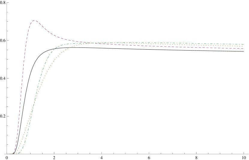
Figure 1: The heat capacity per particle for a system of $n$ fermions; $n=1$ : solid line; $n=2$ : dashed; $n=3$ : dotted; $n=4$ : dot - dashed.

References

- [1] M. Toutounji, Int. J. Quant. Chem. 111, 3475 (2011).
- [2] R. P. Lungu, to appear in Int. J. Quant. Chem.
- [3] A. Messiah, Quantum Mechanics, Ch XII, Sect. 12, North-Holland Publishing House, 1999.
- [4] R. Kubo, H. Ichimura, T. Usui, N. Hashitsume: Statistical Mechanics, North-Holland Publishing House, 1990.
- [5] A. Okopinska, J.Phys.:Conf.Ser., 213 012004.
- [6] I. Bloch, J. Dalibard, W. Zwerger, Rev.Mod.Phys. 80, 885 (2008).
- [7] A. Okopinska, Phys.Rev.D36, 1273 (1987).
- [8] R. P. Feynman, H. Kleinert, Phys.Rev.A34, 5080 (1986).
- [9] Ch. Kittel, Introduction to Solid State Physics, 7th edition, John Wiley & Sons, 1996.
- [10] W. A. Harrison, Applied Quantum Mechanics, World Scientific (2000), exercise 2.2, p.323.
- [11] S. Flugge S.: Practical Quantum Mechanics, vol. 1, problem 18; Springer, 1971.
- [12] http://functions.wolfram.com