Embedded Zassenhaus Expansion to Operator Splitting Schemes: Theory and Application in Fluid Dynamics

Abstract

In this paper, we contribute operator-splitting methods improved by the Zassenhaus product for the numerical solution of linear partial differential equations. We address iterative splitting methods, that can be improved by means of the Zassenhaus product formula, which is a sequnential splitting scheme. The coupling of iterative and sequential splitting techniques are discussed and can be combined with respect to their compuational time. While the iterative splitting schemes are cheap to compute, the Zassenhaus product formula is more expensive, based on the commutators but achieves higher order accuracy. Iterative splitting schemes and also Zassenhaus products are applied in physics and physical chemistry are important and are predestinated to their combinations of each benefits. Here we consider phase models in CFD (computational fluid dynamics). We present an underlying analysis for obtaining higher order operator-splitting methods based on the Zassenhaus product.

Computational benefits are given with sparse matrices, which arose of spatial discretization of the underlying partial differential equations. While Zassenhaus formula allows higher accuracy, due to the fact that we obtain higher order commutators, we combine such an improved initialization process to cheap computable to linear convergent iterative splitting schemes.

Theoretical discussion about convergence and application examples are discussed with CFD problems.

Keywords. Operator splitting method, Iterative splitting, Zassenhaus product, Parabolic differential equations, Convection-Diffusion-Reaction Equations.

AMS subject classifications. 80A20, 80M25, 74S10, 76R50, 35J60, 35J65, 65M99, 65Z05, 65N12.

1  Introduction

Our motivation to study the operator splitting methods come from models in fluid dynamics problems, for example problems in bio-remediation [1] or radioactive contaminants [4], [3].

While standard splitting methods deal with lower order convergence, we propose to a combination of iterative splitting methods with embedded Zassenhaus product formula.

Theoretically, we combine fix-point schemes (iterative splitting methods) with sequential splitting schemes (Zassenhaus products), which are connected to the theory of Lie groups and Lie algebras. Based on that relation, we can construct higher order splitting schemes for an underlying Lie algebra and improve the convergence results with cheap iterative schemes.

Historically, the efficiency of decoupling different physical processes into more simpler processes, e.g., convection and reaction, helps to accelerate the solver process and is discussed in [18].

We propose the following ideas:

• Iterative splitting schemes are based on fix-point schemes, e.g. Waveform relaxation, which linearly improve the convergence order. Based on reducing integral operators to cheap computable matrices, they can be seen as solver methods, see [11].

• Zassenhaus formula are based on nested commutators, which are main keys to derive higher order standard splitting schemes (e.g. Lie-Trotter and Strang splitting). They are simple to compute with their nil-potent structure, see [10].

In this paper we study the following mathematical equations: The equations are coupled with the reaction terms and are presented as follows.

$$\partial_{t}R_{i}u_{i}+\nabla\cdot{\bf v}\;u_{i}=-\lambda_{i}\;R_{i}\;u_{i}+\lambda_{i-1}\;R_{i-1}\;u_{i-1}$$ (1)

$$+\beta(-u_{i}+g_{i})\;\;\mbox{in}\;\Omega\times(0,T)\;,$$

$$u_{i,0}(x)=u_{i}(x,0)\;\;\mbox{on}\;\Omega\;,$$ (2)

$$\partial_{t}R_{i}g_{i}=-\lambda_{i}\;R_{i}\;g_{i}+\lambda_{i-1}\;R_{i-1}\;g_{i-1}$$ (3)

$$+\beta(-g_{i}+u_{i})\;\;\mbox{in}\;\Omega\times(0,T)\;,$$

$$g_{i,0}(x)=g_{i}(x,0)\;\;\mbox{on}\;\Omega\;,$$ (4)

$$i=1,\ldots,m\;,$$

where $m$ is the number of equations and $i$ is the index of each component. The unknown mobile concentrations $u_{i}=u_{i}(x,t)$ are considered in $\Omega\times(0,T)\subset\mathbb{R}^{n}\times\mathbb{R}^{+}$, where $n$ is the spatial dimension. The unknown immobile concentrations $g_{i}=g_{i}(x,t)$ are considered in $\Omega\times(0,T)\subset\mathbb{R}^{n}\times\mathbb{R}^{+}$, where $n$ is the spatial dimension. The retardation factors $R_{i}$ are constant and $R_{i}\geq 0$. The kinetic part is given by the factors $\lambda_{i}$. They are constant and $\lambda_{i}\geq 0$. For the initialization of the kinetic part, we set $\lambda_{0}=0$. The kinetic part is linear and irreversible, so the successors have only one predecessor. The initial conditions are given for each component $i$ as constants or linear impulses. For the boundary conditions we have trivial inflow and outflow conditions with $u_{i}=0$ at the inflow boundary. The transport part is given by the velocity ${\bf v}\in\mathbb{R}^{n}$ and is piecewise constant, see [5] and [6]. The exchange between the mobile and immobile part is given by $\beta$.

The outline of the paper is as follows. The splitting-methods are discussed in Section 2. In Section 3, we present the numerical experiments and the benefits of the higher order splitting methods. Finally, we discuss future work in the area of iterative and non-iterative splitting methods.

2  Operator splitting methods

We focus our attention on the case of two linear operators (i.e., we consider the Cauchy problem):

$$\frac{\partial c(t)}{\partial t}=Ac(t)\;+\;Bc(t),\;\mbox{with}\;t\in[0,T],\;c(0)=c_{0},$$ (5)

whereby the initial function $c_{0}$ is given and $A$ and $B$ are assumed to be bounded linear operators in the Banach-space $\mathbf{X}$ with $A,B:\mathbf{X}\rightarrow\mathbf{X}$. In realistic applications the operators correspond to physical operators such as convection and diffusion operators. We consider the following operator splitting schemes:

2.1  Iterative Operator Splitting

Iterative splitting with respect to one operator

$$\frac{\partial c_{i}(t)}{\partial t}=Ac_{i}(t)\;+\;Bc_{i-1}(t),\;\mbox{with}\;\;c_{i}(t^{n})=c^{n},i=1,2,\ldots,m\;$$ (6)

Theorem 1. 

Let us consider the abstract Cauchy problem given in (5). Then, we the one-side iterative operator splitting method (6) has the following accuracy:

$$||(S_{i}-\exp((A+B)\tau)||\leq C\tau^{i},$$ (7)

where $S_{i}$ is the approximated solution for the i-th iterative step and $C$ is a constant that can be chosen uniformly on bounded time intervals.

Proof.

The proof is done for $i=1,2,\ldots$ and with the consistency error the $e_{i}(\tau)=c(\tau)-c_{i}(\tau)$ we have :

$$c_{i}(\tau)=\exp(A\tau)c(t^{n})$$ (8)

$$+\int_{t^{n}}^{t^{n+1}}\exp(A(t^{n+1}-s))B\exp(sA)c(t^{n})\;ds$$

$$+\int_{t^{n}}^{t^{n+1}}\exp(A(t^{n+1}-s_{1}))B\int_{t^{n}}^{t^{n+1}-s_{1}}\exp((t^{n+1}-s_{1}-s_{2})A)B\exp(s_{2}A)c(t^{n})\;ds_{2}\;ds_{1}$$

$$+\ldots$$

$$+\int_{t^{n}}^{t^{n+1}}\exp(A(t^{n+1}-s_{1}))B\int_{t^{n}}^{t^{n+1}-s_{1}}\exp((t^{n+1}-s_{1}-s_{2})A)B\exp(s_{2}A)c(t^{n})\;ds_{2}\;ds_{1}+\ldots$$

$$+\int_{t^{n}}^{t^{n+1}}\exp(A(t^{n+1}-s_{1}))B$$

$$\ldots\int_{t^{n}}^{t^{n+1}-\sum_{j=1}^{i-2}s_{j}}\exp((t^{n+1}-\sum_{j=1}^{i-1}s_{j})A)Bc_{init}(s_{i})\;ds_{i}\;ds_{i-1}\ldots\;ds_{2}\;ds_{1},$$

$$c(\tau)=\exp(A\tau)c(t^{n})$$ (9)

$$+\int_{t^{n}}^{t^{n+1}}\exp(A(t^{n+1}-s))B\exp(sA)c(t^{n})\;ds$$

$$+\int_{t^{n}}^{t^{n+1}}\exp(A(t^{n+1}-s_{1}))B\int_{t^{n}}^{t^{n+1}-s_{1}}\exp((t^{n+1}-s_{1}-s_{2})A)B\exp(s_{2}A)c(t^{n})\;ds_{2}\;ds_{1}$$

$$+\ldots$$

$$+\int_{t^{n}}^{t^{n+1}}\exp(A(t^{n+1}-s_{1}))B\int_{t^{n}}^{t^{n+1}-s_{1}}\exp((t^{n+1}-s_{1}-s_{2})A)B\exp(s_{2}A)c(t^{n})\;ds_{2}\;ds_{1}$$

$$+\ldots+\int_{t^{n}}^{t^{n+1}}\exp(A(t^{n+1}-s_{1}))B$$

$$\ldots\int_{t^{n}}^{t^{n+1}-\sum_{j=1}^{i-1}s_{j}}\exp((t^{n+1}-\sum_{j=1}^{i}s_{j})A)B\exp((s_{i}(A+B))c(t^{n})\;ds_{i}\ldots\;ds_{2}\;ds_{1},$$

We obtain:

$$||e_{i}||\leq||\exp((A+B)\tau)c(t^{n})-S_{i}(\tau)c_{init}(\tau)||$$

$$\leq C\tau^{i}\max_{s_{i}\in[0,\tau]}||\exp((s_{i}(A+B))c(t^{n})-c_{init}(s_{i})||$$

$$\leq C\tau^{i}||\exp((\tau(A+B))c(t^{n})-c_{init}(\tau)||,$$ (10)

where $i$ is the number of iterative steps.

The same idea can be applied to the even iterative scheme and also for alternating $A$ and $B$.

∎

Remark 1.

The accuracy of the initialisation $c_{init}(\tau)$ is important to conserve or improve the underlying iterative splitting scheme.

Here we have the following initialization schemes:

$$c_{i}(\tau)=\exp(A\tau)c(t^{n})\rightarrow||e_{i}||\leq C\tau^{i}c(t^{n}),$$ (11)

$$c_{i}(\tau)=\exp(A\tau)\exp(B\tau)c(t^{n})\rightarrow||e_{i}||\leq C\tau^{i+1}c(t^{n}).$$ (12)

2.2  Zassenhaus formula (Sequential Splitting)

The Zassenhaus formula is an extension to the exponential splitting schemes and is given as:

$$\exp((A+B)t)=\pi_{i=1}^{j}\exp(a_{i}At)\exp(b_{i}Bt)\pi_{k=j}^{m}\exp(C_{k}t^{k})+O(t^{m+1}).$$ (13)

where $C_{j}$ is a function of Lie brackets of $A$ and $B$.

Theorem 2. 

The initial value problem (5) is solved by classical exponential splitting schemes.

Then we can embed the Zassenhaus formula and improve the classical splitting schemes

$$\exp((A+B)t)=\pi_{i=1}^{j}\exp(a_{i}At)\exp(b_{i}Bt)\pi_{k=j}^{m}\exp(C_{k}t^{k})+O(t^{m+1}).$$ (14)

where $C_{j}$ is a function of the Lie brackets of $A$ and $B$.

Proof.

1.) Lie-Trotter splitting:

For the Lie-Trotter splitting there exists coefficients with respect to the extension:

$$\exp((A+B)t)=\exp(At)\exp(Bt)\Pi_{k=2}^{\infty}\exp(C_{k}t^{k}),$$ (15)

where the coefficients $C_{k}$ are given in [10].

Based on an existing Baker-Campbell-Hausdorff (BCH) formula of the Lie-Trotter splitting one can apply the Zassenhaus formula.

2.) Strang Splitting:

A existing BCH formula is given as:

$$\exp(At/2)\exp(Bt)\exp(At/2)=\exp(tS_{1}+t^{3}S_{3}+t^{5}S_{5}+\ldots),$$ (16)

where the coefficients $S_{i}$ are given as in [12].

There exists a Zassenhaus formula based on the BCH formula:

$$\exp((A/2+B/2)t)=\Pi_{k=2}^{\infty}\exp(\tilde{C}_{k}t^{k})\exp(A/2t)\exp(B/2t),$$ (17)

and

$$\exp((B/2+A/2)t)=\exp(B/2t)\exp(A/2t)\Pi_{k=2}^{\infty}\exp(C_{k}t^{k}),$$ (18)

then there exists a new product:

$$\Pi_{k=3}^{\infty}\exp(D_{k}t^{k})=\Pi_{k=2}^{\infty}\exp(\tilde{C}_{k}t^{k})\Pi_{k=2}^{\infty}\exp(C_{k}t^{k}),$$ (19)

with one order higher, see also [22].

∎

Remark 2.

In the following, we concentrate on the Lie-Trotter splitting with the embedded Zassenhaus formula, given as:

$$E_{Zassen,Comp,1}(t)=\exp(At)\exp(Bt),$$ (20)

$$E_{Zassen,Comp,j}(t)=\exp(C_{j}t^{j}),\mbox{for}\;j\in 2\ldots,i,$$ (21)

where the sequential Zassenhaus operator

$$E_{Zassen,i}(t)=\Pi_{j=1}^{i}E_{Zassen,Comp,j}(t),$$ (22)

is of accuracy $O(t^{i})$ and $i$ are the number of Zassenhaus components.

2.3  Embedding Zassenhaus expansion to Iterative Splitting schemes

In the following we discuss the embedding of the Zassenhaus formula into the iterative operator splitting schemes.

Theorem 3. 

We solve the initial value problem (5). We assume bounded and constant operators $A$, $B$.

The initialization process is done with the Zassenhaus formula:

$$c_{i}(t)=E_{Zassen,i}(t)c_{0}.$$ (23)

where $E_{Zassen,i}(t)$ is given in (22).

Further the improved solutions are embedded to the iterative splitting schemes (6) and we have after $j$ iterative steps the following result:

$$c_{i+j}(t)=E_{iter,j}(t)E_{Zassen,i}(t)c_{0}.$$ (24)

where we can improve the error of the iterative scheme to $\mathcal{O}(t^{i+j})$.

Proof.

The solution of the iterative splitting scheme (6) is given as:

$$c_{i+j}(t)=E_{iter,i}(t)c_{init,j}.$$ (25)

where $S_{i}(t)=E_{iter,i}(t)$.

The initialization is given with the Zassenhaus formula as:

$$c_{init,j}(t)=E_{Zassen,j}(t)c_{0}.$$ (26)

combining both splitting schemes we have the local error:

$$e_{i+j}(t)=||c(t)-c_{i+j}(t)||=||c(t)-E_{iter,i}(t)E_{Zassen,j}(t)c_{0}||\leq O(t^{i+j})c_{0}.$$ (27)

∎

3  Numerical Examples

In this section, we discuss examples to the usage of the embedded Zassenhaus product methods to the iterative splitting schemes. In the first examples, we demonstrate somewhat artificially how the proposed Zassenhaus splitting method avoids the splitting error up to a certain order. The next examples show the solution of partial differential equation which can be improved by the Zassenhaus products.

In the following, we deal with numerical example to verify the theoretical results.

3.1  First Example: Matrix problem

For another example, consider the matrix equation,

$$u^{\prime}(t) = \left[\begin{array}[]{cc}1&2\\ 3&0\\ \end{array}\right]u,\,\,\,\,\,\,u(0)=u_{0}=\left(\begin{array}[]{c}0\\ 1\\ \end{array}\right),$$ (32)

the exact solution is

$$u(t) = 2(e^{3t}-e^{-2t})/5.$$ (33)

We split the matrix as,

$$\left[\begin{array}[]{cc}1&2\\ 3&0\\ \end{array}\right] = \left[\begin{array}[]{cc}1&1\\ 1&0\\ \end{array}\right]+\left[\begin{array}[]{cc}0&1\\ 2&0\\ \end{array}\right]$$ (40)

The Figure 1 present the numerical errors between the exact and the numerical solution.

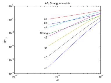
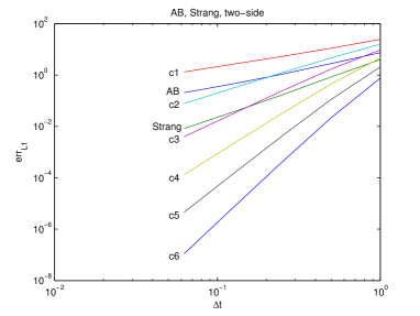
Figure 1: Numerical errors of the standard Splitting scheme and the iterative schemes with $1,\ldots,6$ iterative steps.

The Figure 2 present the CPU time of the standard and the iterative splitting schemes.

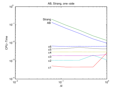
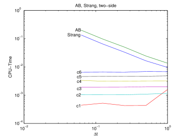
Figure 2: CPU time of the standard Splitting scheme and the iterative schemes with $1,\ldots,6$ iterative steps.

Remark 3.

We see that the errors decrease significantly with increasing order of approximation for the initialization process with the Zassenhaus splitting. Here we have the benefit in the application of the Zassenhaus product schemes to the standard Lie-Trotter or Strang-Marchuk splitting. Similar results are given with the iterative steps $i=3\ldots,6$, as expected.

3.2  One phase example

The next example is a simplified real-life problem for a multiphase transport-reaction equation. We deal with mobile and immobile pores in the porous media, such simulations are given for waste scenarios.

We concentrate on the computational benefits of a fast computation of the mixed iterative scheme with the Zassenhaus formula.

The one phase equation is given as:

$$\partial_{t}c_{1}+\nabla\cdot{\bf F}c_{1}=-\lambda_{1}c_{1},\;\mbox{in}\;\Omega\times[0,t],$$ (41)

$$\partial_{t}c_{2}+\nabla\cdot{\bf F}c_{2}=\lambda_{1}c_{1}-\lambda_{2}c_{2},\;\mbox{in}\;\Omega\times[0,t],$$ (42)

$${\bf F}={\bf v}-D\nabla,$$ (43)

$$c_{1}({\bf x},t)=c_{1,0}({\bf x}),c_{2}({\bf x},t)=c_{2,0}({\bf x}),\;\mbox{on}\;\Omega,$$ (44)

$$c_{1}({\bf x},t)=c_{1,1}({\bf x},t),c_{2}({\bf x},t)=c_{2,1}({\bf x},t),\;\mbox{on}\;\partial\Omega\times[0,t].$$ (45)

where we have the parameters: $v=0.1$, $D=0.01$, $\lambda_{1}=\lambda_{2}=0.1$.

In the following we deal with the finite difference schemes for the convection and diffusion operators and semidiscretize the equation, which is given as:

$$\partial_{t}{\bf c}=(A_{1}+A_{2}){\bf c},$$ (46)

We obtain the two matrices and consider to decouple the diffusion and convection part:

$$A_{1} = \left(\begin{array}[]{c c}A_{diff}&0\\ 0&A_{diff}\end{array}\right)~{}\in~{}\mathbb{R}^{2I\times 2I}$$ (49)

$$A_{2} = \left(\begin{array}[]{c c}A_{Conv}&0\\ 0&A_{Conv}\end{array}\right)+\left(\begin{array}[]{c c}-\Lambda_{1}&0\\ \Lambda_{1}&-\Lambda_{2}\end{array}\right)~{}\in~{}\mathbb{R}^{2I\times 2I}$$ (54)

For the operator $A_{1}$ and $A_{2}$ we apply the splitting method, given in Section LABEL:para.

The submatrices are given in the following:

$$A = \left(\begin{array}[]{c c}A_{diff}&0\\ 0&A_{diff}\end{array}\right)+\left(\begin{array}[]{c c}A_{conv}&0\\ 0&A_{conv}\end{array}\right)$$ (59)

$$= \frac{D}{\Delta x^{2}}\cdot\left(\begin{array}[]{rrrrr}-2&1&{}\hfil&{}\hfil&{}\hfil\\ 1&-2&1&{}\hfil&{}\hfil\\ {}\hfil&\ddots&\ddots&\ddots&{}\hfil\\ {}\hfil&{}\hfil&1&-2&1\\ {}\hfil&{}\hfil&{}\hfil&1&-2\end{array}\right)$$ (65)

$$- \frac{v}{\Delta x}\cdot\left(\begin{array}[]{rrrrr}1&{}\hfil&{}\hfil&{}\hfil&{}\hfil\\ -1&1&{}\hfil&{}\hfil&{}\hfil\\ {}\hfil&\ddots&\ddots&{}\hfil&{}\hfil\\ {}\hfil&{}\hfil&-1&1&{}\hfil\\ {}\hfil&{}\hfil&{}\hfil&-1&1\end{array}\right)~{}\in~{}\mathbb{R}^{I\times I}$$ (71)

where $I$ is the number of spatial points and $\Delta x$ is the spatial step size.

$$\Lambda_{1} = \left(\begin{array}[]{rrrrr}\lambda_{1}&0&{}\hfil&{}\hfil&{}\hfil\\ 0&\lambda_{1}&0&{}\hfil&{}\hfil\\ {}\hfil&\ddots&\ddots&\ddots&{}\hfil\\ {}\hfil&{}\hfil&0&\lambda_{1}&0\\ {}\hfil&{}\hfil&{}\hfil&0&\lambda_{1}\end{array}\right)~{}\in~{}\mathbb{R}^{I\times I}$$ (77)

$$\Lambda_{2} = \left(\begin{array}[]{rrrrr}\lambda_{2}&0&{}\hfil&{}\hfil&{}\hfil\\ 0&\lambda_{2}&0&{}\hfil&{}\hfil\\ {}\hfil&\ddots&\ddots&\ddots&{}\hfil\\ {}\hfil&{}\hfil&0&\lambda_{2}&0\\ {}\hfil&{}\hfil&{}\hfil&0&\lambda_{2}\end{array}\right)~{}\in~{}\mathbb{R}^{I\times I}$$ (83)

We have the following results:

We have the spatial step size $\Delta x=0.1$.

The Figure 3 present the numerical errors between the exact and the numerical solution.

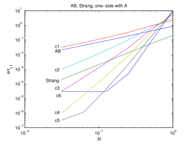
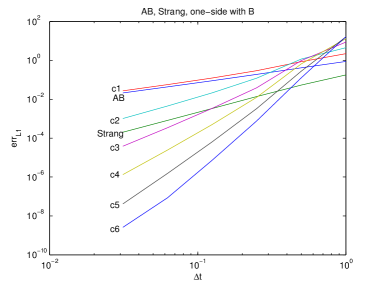
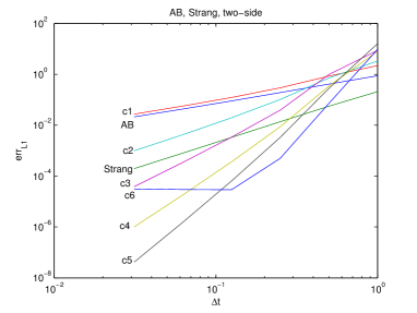
Figure 3: Numerical errors of the standard Splitting scheme and the iterative schemes with $1,\ldots,6$ iterative steps.

The Figure 4 present the CPU time of the standard and the iterative splitting schemes.

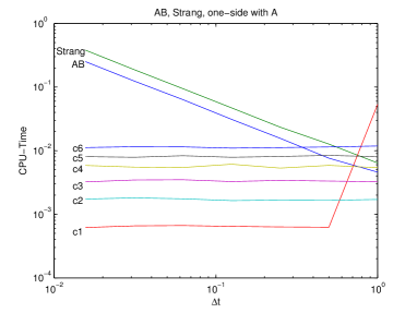
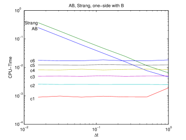
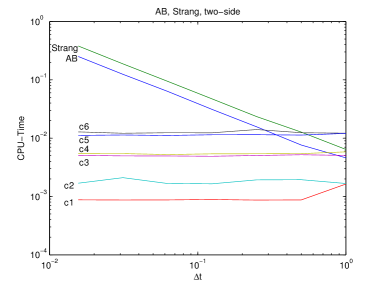
Figure 4: CPU time of the standard Splitting scheme and the iterative schemes with $1,\ldots,6$ iterative steps.

Remark 4.

For the iterative schemes with embedded Zassenhaus products, we can reach faster and more improved results. With $4-5$ iterative steps we obtain more accurate results as we did for the expensive standard schemes. With one-side iterative schemes we reach the best convergence results.

4  Conclusions and Discussions

In this work, we have presented a novel splitting scheme combing the ideas of iterative and sequential schemes. Here the idea to decouple the expensive computation of only matrix exponential based schemes to simpler embedded Zassenhaus schemes, which have their benefits of less computational time, while the commutator can be computed very cheap. On the other hand simple linear iterative steps can be done very cheap and accelerated the solvers. The error analysis presented stable methods for the higher order schemes. In the applications, we could show the speedup with the Zassenhaus enhanced methods. In future we concentrate on linear and nonlinear matrix dependent scheme, that switches between no-iterative and iterative schemes based on Zassenhaus products.

References

• [1] R.E. Ewing. Up-scaling of biological processes and multiphase flow in porous media. IIMA Volumes in Mathematics and its Applications vol. 295, Springer, New York, 2002, pp. 195–215.
• [2] I. Farago, J. Geiser. Iterative Operator-Splitting methods for Linear Problems. Preprint No. 1043 of the Weierstrass Institute for Applied Analysis and Stochastics, Berlin, June 2005.
• [3] P. Frolkovič and J. Geiser. Numerical Simulation of Radionuclides Transport in Double Porosity Media with Sorption. Proceedings of Algorithmy 2000, Conference of Scientific Computing, 2000, pp. 28–36.
• [4] J. Geiser. Numerical Simulation of a Model for Transport and Reaction of Radionuclides. Proceedings of the Large Scale Scientific Computations of Engineering and Environmental Problems, Sozopol, Bulgaria, 2001.
• [5] J. Geiser. Gekoppelte Diskretisierungsverfahren für Systeme von Konvektions-Dispersions-Diffusions-Reaktionsgleichungen. Doktor-Arbeit, Universität Heidelberg, 2003.
• [6] J. Geiser. $R^{3}T$: Radioactive-Retardation-Reaction-Transport-Program for the simulation of radioactive waste disposals. Proceedings: Computing, Communications and Control Technologies: CCCT 2004, The University of Texas at Austin and The International Institute of Informatics and Systemics (IIIS) 2004, to appear.
• [7] J. Geiser. Iterative Operator-Splitting Methods with higher order Time-Integration Methods and Applications for Parabolic Partial Differential Equations. Journal of Computational and Applied Mathematics, Elsevier, Amsterdam, The Netherlands, 217, 227-242, 2008.
• [8] J. Geiser. Decomposition Methods for Differential Equations: Theory and Applications. Chapman & Hall/CRC Press, Numerical Analysis and Scientific Computing, F. Magoules and Ch.-H. Lai, eds., 2009.
• [9] J. Geiser and G. Tanoglu. Operator-splitting methods via Zassenhaus product formula. Applied Mathematics and Computation, vol. 217, 4557-4575, 2011.
• [10] J. Geiser, G. Tanoglu and N. Guecueyenen. Higher Order Operator-Splitting Methods via Zassenhaus product formula: Theory and Applications. Computers and Mathematics with Applications, Elsevier, North Holland, 62(4)1994-2015, 2011.
• [11] J. Geiser. Computing Exponential for Iterative Splitting Methods. Journal of Applied Mathematics, special issue: Mathematical and Numerical Modeling of Flow and Transport (MNMFT), Hindawi Publishing Corp., New York, accepted, January 2011.
• [12] E. Hairer, C. Lubich and G. Wanner. Geometric Numerical Integration. Springer Series in Computational Mathematics, vol. 31, Springer Verlag, Berlin, 2002.
• [13] W.H. Hundsdorfer, J. Verwer. Numerical solution of time-dependent advection-diffusion-reaction equations, Springer, Berlin, 2003.
• [14] J. Kanney, C. Miller, and C.  Kelley. Convergence of iterative split-operator approaches for approximating nonlinear reactive transport problems. Advances in Water Resources, 26(2003):247–261.
• [15] R.J. LeVeque. Finite Volume Methods for Hyperbolic Problems. Cambridge Texts in Applied Mathematics, Cambridge University Press, 2002.
• [16] X. Lu, Y. Sun and J.N.  Petersen. Analytical solutions of TCE transport with convergent reactions. Transport in porous media, 51(2003):211–225.
• [17] G.I  Marchuk. Some applicatons of splitting-up methods to the solution of problems in mathematical physics. Aplikace Matematiky, 1(1968):103–132.
• [18] R.I. McLachlan, G. Reinoult, and W. Quispel. Splitting methods. Acta Numerica, (2002):341–434.
• [19] J.A. Oteo. The Baker-Campbell-Hausdorff formula and nested commutator identities. Journal of Mathematical Physics, 32(1991):419.
• [20] G. Strang. On the construction and comparision of difference schemes. SIAM J. Numer. Anal., 5(1968):506–517.
• [21] S. Vandewalle. Parallel Multigrid Waveform Relaxation for Parabolic Problems. Teubner, Stuttgart, 1993.
• [22] H. Yoshida. Construction of higher order symplectic integrators Physics Letters A, Vol. 150(1990), nos. 5–7.
• [23] M. Suzuki. On the convergence of exponential operators – the Zassenhaus formula, BCH formula and systematic approximants. Commun. Math. Phys., vol. 57, 193–200, 1977.
• [24] M. Suzuki. General theory of fractal path integrals with applications to many-body theories and statistical physics. J. Math. Phys., vol. 32, 400–407, 1991.