Nonlinear Wave Interactions as Emission Process of Type II Radio Bursts

Abstract

The emission of fundamental and harmonic frequency radio waves of type II radio bursts are assumed to be products of three-wave interaction processes of beam-excited Langmuir waves. Using a particle-in-cell code, we have performed simulations of the assumed emission region, a CME foreshock with two counterstreaming electron beams. Analysis of wavemodes within the simulation shows self-consistent excitation of beam driven modes, which yield interaction products at both fundamental and harmonic emission frequencies. Through variation of the beam strength, we have investigated the dependence of energy transfer into electrostatic and electromagnetic modes, confirming the quadratic dependence of electromagnetic emission on electron beam strength.

1 Overview

Emission of radio bursts from the solar corona has been observed since the early 1950ies (Wild & McCready, 1950). While theoretical explanations for the emission mechanisms of most types of bursts have been found, many details of the emission process of type II radio bursts are still a matter of discussion.

The morphology of type II bursts typically shows a two-band emission spectrum, consisting of the fundamental emission band and of the harmonic emission band at about twice the frequency of the fundamental (in a few, near-limb events signals of third harmonic emission are also discernable, see Zlotnik et al., 1998). The fundamental frequency is believed to correspond to the plasma frequency of the emission region, slowly decreasing over time as the coronal/interplanetary shock travels outwards into the heliosphere. (Cane et al., 1987; Nelson & Melrose, 1985)

The commonly accepted model by Reiner et al. (1998) proposes that the emission region is located around points where the CME drives a curved perpendicular shock, leading to efficient shock drift acceleration of electrons. Due to the curved nature of the shock, these can escape into the foreshock following the magnetic field, where they form an electron beam population. This model has been thoroughly treated analytically. Knock et al. (2001) have derived theoretical emissivities for Langmuir wave emission and subsequent conversion into electromagnetic emissions, and Schmidt & Gopalswamy (2008) have combined these with MHD simulations to track the radio burst emission region as it moves outward from the Sun. These theoretical predictions are however not in complete agreement with observations, and many details of the fine structure (band splitting and herringbone patterns) often visible on type II bursts are yet to be explained(Aurass et al., 1994).

Similar to the assumed emission process of type III bursts, instabilities driven by the electron beams can then lead to creation of Langmuir waves $(L)$ and their three wave interaction products (Ion-soundwaves $S$ and transverse electromagnetic waves $T$) (Melrose, 1986):

$$L \rightarrow L^{\prime}+S$$ (1)

$$L \rightarrow S+T(\omega_{pe})$$ (2)

$$L+L^{\prime} \rightarrow T(2\omega_{pe})$$ (3)

Momentum and energy conservation as well as wave polarization impose certain limits on the waves’ $\vec{k}$ directions (Spanier & Vainio, 2009). The Langmuir waves (L) should primarily be excited parallel to the beam direction, potentially following the beam electrons’ pitch angle distribution (Karlický & Vandas, 2007), whereas electromagnetic waves are expected to be emitted in quasi-perpendicular directions: Assuming that

$$k^{L}_{\parallel} = k_{\parallel}^{T}+k_{\parallel}^{S}$$ (4)

$$k^{L}_{\perp} = k_{\perp}^{T}+k_{\perp}^{S}$$ (5)

$$\omega^{L} = \omega^{T}+\omega^{S},$$ (6)

Angular momentum conservation leads to polarization selection rules (Spanier & Vainio, 2009). Inserting the dispersion relations for all three waves and using these selection rules to neglect $k_{\parallel}^{T}$ as well as $k_{\perp}^{S}$, we get

$$3k_{\parallel}^{2}v^{2}_{\mathrm{th}}=c^{2}k_{\perp}^{2}+k_{\parallel}^{2}v_{s}^{2}+2k_{\parallel}v_{s}\omega_{pe}+k_{\perp}k_{\parallel}v_{s}c,$$ (7)

(with speed of sound $v_{s}$ and electron thermal speed $v_{\mathrm{th}}$) which results in an expected $k$-value for the harmonic electromagnetic emission of

$$k_{\perp}=-\frac{v_{s}}{2c}k_{\parallel}\pm\sqrt{3k_{\parallel}^{2}\left(\frac{v_{\mathrm{th}}^{2}}{c^{2}}-\frac{v_{s}^{2}}{4c^{2}}\right)-2\frac{v_{s}}{c^{2}}k_{\parallel}\omega_{pe}}.$$ (8)

Being a second-order coupling of Langmuir waves, the intensity of the electromagnetic emission is expected to be quadratic in the Langmuir wave energy, and should thus also be quadratic in the initial electron beam energy (Knock et al., 2001) for the model described here. This assumes a fixed level of ion soundwave intensity, which the simulations in this work provide through identical thermal initialization of the background ion population in all runs. Excitation of additional soundwave intensity by the beam can be neglected due to the small simulation timescales.

In the simplest case of this emission scenario, a single electron beam emission site, created on a smoothly curved CME shock, is supplying the electron beam populations for radio emission. Langmuir waves excited through the beam driven instability would first have to scatter off soundwaves (Eq. 1) at a sufficient rate to create a suitable population of counter-propagating Langmuir waves $L^{\prime}$. If this process is too slow, harmonic emission (Eq. 3) cannot be expected to attain intensities which are comparable to the fundamental plasma emission process.

An alternative scenario can be constructed by assuming not one single, but two (or multiple) points along a shock front in which perpendicular shock conditions pertain, allowing for drift acceleration of electrons into the foreshock. This could be caused by shock ripples at the front of the CME, or density fluctuations in the background solar wind leading to inhomogeneous propagation of the shock through the heliosphere. With multiple electron acceleration sites feeding electron beams into the foreshock from different directions, counterstreaming electron beams may be present within the emission region. Direct excitation of counter-propagating Langmuir waves through beam driven instability is hence possible, leading to a stronger harmonic emissivity.

Due to the relatively small size of the emission region, in-situ satellite observation data is very scarce. In a handful of cases however, measurements of interplanetary type II burst emission regions were possible, as an outward-expanding CME shock front encountered spacecraft at 1AU(Pulupa & Bale, 2008). The measurements obtained from these emission-region crossings agree with the proposed model, in that they provide evidence of counterstreaming foreshock electron beam presence. Electric field measurements on board the spacecraft are also indicating a strong presence of waves near the plasma frequency, attributed to Langmuir waves. However, direct in-situ satellite measurements of wave quantities are limited to the resolution of $\omega_{s}$ in the spacecraft’s frame. Since the solar wind is streaming by the spacecraft at a velocity $\vec{u}_{sw}$, this quantity is a mixture of $\omega_{s}=\omega+\vec{u}_{sw}\cdot\vec{k}$, but the $k$ contribution is negligible for the high-frequency wavemodes of interest to this study. While multispacecraft observations have been successful in reconstructing directionalities of radio bursts (Thejappa et al., 2012), a detailed analysis of the kinematics of three wave interaction processes, for which information with both $\omega$ and $\vec{k}$ resolution is essential, can only be provided by simulations.

1.1 Related Work

In similar work, Karlický & Vandas (2007) performed 1.5D simulations of beam-excitation of Langmuir waves from foreshock electrons, and subsequent couplings to kinetic wavemodes. Due to the limitation to one spatial dimension, these runs were not able to represent waves with transverse momentum and hence precluded the subsequent electromagnetic emission mechanism (eqs. 2, 3). In Karlicky & Barta (2010), 2.5D PiC simulations were conducted into which monochromatic, coherent Langmuir waves were artificially injected as an initial condition instead of an electron beam, yielding a strong signal of both fundamental and harmonic emission. Yu & Guangli (2008) focused on the generation of backward-propagating waves through scattering (Eq.1), confirming that direct creation of these waves is difficult in a particle-in-cell simulation. Finally, the simulations of J. I. Sakai & M. Karlický (2008) attempt to model the shock structure itself within the simulation box, in an attempt to represent the complete emission mechanism within one self-contained simulation. Due to the inherent numerical limits given by a PiC code, both the accelerated particles and wave quantities are at odds with the other papers presented here.

2 Simulation

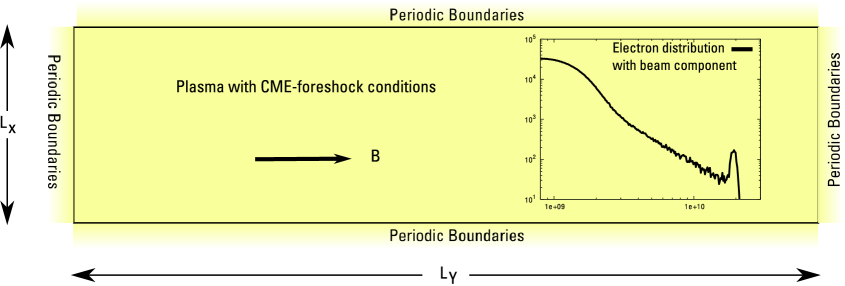
Figure 1: Numerical simulation setup of the 2.5D PiC simulations. In addition to the homogeneous, thermal background plasma, two counterstreaming electron beam populations are present.

Since the phenomenology of beam-driven wave instabilities depends on an electron distribution function that is far from equilibrium, MHD or fluid simulations are not suitable for this problem, but rather kinetic simulation methods have to be employed, with correspondingly larger computational requirements. To obtain and analyze full spatial information about wave processes within the CME foreshock region (as opposed to 1D satellite measurements), the kinetic particle-in-cell simulation code ACRONYM (Kilian et al., 2012) was used. This code, developed and maintained at the Department of Astronomy, University of Würzburg, is a fully relativistic, 2nd order particle-in-cell code for astronomical, heliospheric and laboratory plasmas. Using MPI-parallelization, the code is running on all major supercomputing platforms.

Due to the inherent length- and timescale requirements (governed by the plasma Debye length of about $\lambda_{D}\approx 1\,\mathrm{cm}$) of kinetic simulations, it is impossible to model a complete CME, or even a significant part of the actual shock front within the bounds of a simulation. Rather, the microphysics of plasma wave interaction within the foreshock region is of central importance here. The actual simulations therefore model only the foreshock region, with the electron beam initialized as external input.

Improving on earlier work (Ganse et al., 2011b), the focus of this paper is the self-consistent creation of electromagnetic emission from Langmuir waves which have not been artificially created as monochromatic external input, but excited through instabilities within the simulation itself. Correspondingly larger timescales and better spectral resolution are required over Karlicky & Barta (2010). The simulations are set up as 2.5D rectangular grids with periodic boundaries, which are homogeneously filled with the background foreshock plasma under quiescent coronal conditions ($T\approx 1\,\mathrm{MK}$, $\rho=2.5\cdot 10^{7}\mathrm{cm}^{-3}$, $B=1\mathrm{G}$), with a thermal particle distribution. On top of that, two counterstreaming beamed electron populations are added at $v_{\mathrm{Beam}}\approx 5v_{\mathrm{th}}$, whose density is $10\%-15\%$ of the total electron density (see Fig. 1), based on in-situ observation data (Knock et al., 2001). Their pitch angle distribution is centered around $45^{\circ}$, following Karlický & Vandas (2007).

The selection of two counterstreaming electron populations as opposed to a single beam is motivated by our earlier results (Ganse et al., 2011a), as well as work by Yu & Guangli (2008), showing that a creation of backward-propagating Langmuir waves of sufficient strength within a PiC simulation is itself numerically challenging. The counterstreaming beam setup provides symmetric creation of forward- and backward-propagating waves, and can physically occur in scenarios of multiple shock drift acceleration sites (Cairns et al., 2003).

To obtain physically valid results, the electron to proton mass ratio has been chosen as the physical $m_{p}/m_{e}=1836$, the protons being part of the homogeneous, thermal background. In order to reduce the fundamental problem of numerical noise in our PiC-simulations, the particle number per cell had to be chosen quite large. Results have shown that below 100 particles per cell, nonlinear wave interactions were strongly disturbed by nonphysical effects due to statistical noise. This also sets a lower limit to the beam intensities which can be simulated given the current computational resources, as the generated wave signals have to be sufficiently stronger than the noise background. They are however still in reasonable agreement with Knock et al. (2001).

Using large supercomputers, numerical simulation extents of $8192\times 4096$ cells with $200$ particles per cell were attainable, leading to physical extents of $80.28\times 40.14$ metres. While this is still many orders of magnitude smaller than the expected size of the complete emission region, it resolves the kinetic plasma length scales and the wavelengths of all contributing waves with sufficient headroom.

Figure 2: Energy distribution in two foreshock electron beam simulations. A transfer of energy into electric fields and subsequently into transverse magnetic fields is taking place, starting from $t\sim 20\omega_{pe}^{-1}$. In a direct comparison of two simulations with a $50\%$ difference in electron beam density, a $52.7\%$ increase in peak electric field intensity is observed. The resulting gain in magnetic field energy exceeds that, yielding a $172\%$ increase.

Multiple simulation runs were conducted to study the influence of multiple input parameters on the wave interaction behaviour in this scenario: The basic simulation setup outlined above was varied in beam density (a $50\%$ increase) and background plasma density.

3 Results

In the following, the results of two simulation runs, one with electron beam density $10\%$ of the background plasma density, and one with $15\%$ of background plasma density shall be presented and compared. Firstly, the spatially averaged distribution of energy into particle kinetic energy, electric and magnetic fields will be discussed, followed by decomposition of the field’s energy contributions into individual spatial modes.

The energy distribution within the simulations’ constituents (Fig. 2) yields that the initial energy, stored only in the particles’ motion and the background B-field, starts to convert into electric field energy at around $t=20\omega_{pe}^{-1}$. Soon afterwards, energy conversion into transverse B-field components is also observed.

The initial transfer of energy into electric fields is attributed to the excitation of Langmuir waves by the presence of the electron beam, consistent with theoretical predictions. The peak energy content in the electric field is about $2\%$ of the initial electron beam’s kinetic energy, confirming the results of Karlický & Vandas (2007). The conversion of electric into magnetic energy (in the transverse components of the B-field) is then attributed to the creation of transverse electromagnetic waves.

A direct comparison between the simulation with the weaker electron beams (electron density $n_{\mathrm{beam}}\sim 10\%\;n_{\mathrm{bg}}$) and the stronger-beam simulation ($n_{\mathrm{beam}}\sim 15\%\;n_{\mathrm{bg}}$, same beam velocity), given in Table 1 shows that the increase in beam energy leads to a proportionate increase in peak electric field strength, and a much larger increase in transverse magnetic field energy. The increase in electric field energy by $53\%$ is consistent with the linear relationship of beam strength to electrostatic mode excitation by Cherenkov-type instabilities.

Beam electron density (as $\%$ of $n_{\mathrm{bg}}$)	Peak electric field energy	Peak transverse mag. field energy
10	$1082\,\mathrm{erg}$	$0.18\,\mathrm{erg}$
15	$1652\,\mathrm{erg}$	$0.49\,\mathrm{erg}$
Energy ratio	1.53	2.72

Table 1: Comparison of two simulation runs, in terms of electron beam intensity and resulting energy content in electric and transverse magnetic field components.

If the transverse magnetic field strength is actually caused by second-order wave couplings of electrostatic wavemodes, as outlined in section 8, a quadratic increase in energy in this component relative to the electrostatic mode energy is expected: The observed increase by a factor of $2.72$ is in reasonable agreement with this prediction, as $\sqrt{2.72}=1.65$ is comparable to the growth of the electrostatic mode by a factor of $1.53$. Higher-order nonlinear effects might be the cause for additional energy excess here.

In order to obtain more detailed quantitative information about the energy distribution into different wave modes within the foreshock plasma, the discretized simulation data was Fourier-transformed both in space, allowing analysis of instantaneous k-space spectra, and in time, to obtain dispersion diagrams.

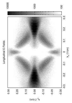
Figure 3: $k$-space distribution of wave energies in the foreshock plasma (arbitrary units). Left: Longitudinal electric field, Right: Transverse magnetic field. The x-axis corresponds to the electron beam direction.

Figure 3 shows $k$-space intensities of longitudinal $E$- and transverse $B$-Fields at $t=65\,\omega_{pe}^{-1}$. The $x$-axis corresponds to the electron streaming direction.

By taking the Fourier transform in both temporal and spatial dimensions, the dispersion plots in Fig. 4 and 5 are obtained. They respectively show the relative intensities of the longitudinal electric and transverse magnetic fields in relation to $\omega$ and $k$.

3.1 Langmuir wave excitation

The longitudinal E-field (Fig. 3, left picture) shows maxima of intensity along the streaming direction, as well as resonant excitations consistent with the streaming electrons’ pitch angle distribution, forming cones of high intensity around the x-axis. An additional, but weaker component perpendicular to the streaming direction is also visible. The cones around the x-axis are the expected signature of beam-driven wave excitation, following the beam direction and being widened by the electrons’ pitch-angle distribution. The components oblique and quasi-perpendicular to the electron beams’ direction are not explained by this mechanism, and are assumed to be scattering products of three-wave interactions, as outlined in Karlicky & Barta (2010).

In Fig. 4, $k_{y}=0$ cuts through $\vec{k}$-space have been taken for both the weak beam and strong beam case, and Fourier-transformed in time to yield $k-\omega$ dispersion diagrams, allowing for identification of individual wave modes. In the right picture, intensity ratios between the weak beam and strong beam simulation are depicted, showing that the added wave intensity primarily leads to a broadening of the beam mode excitation towards lower frequencies. The dominant contribution of energy in these plots is located on the beam mode, with a constant phase velocity matching the average beam velocity (Willes & Cairns, 2000). Around the plasma frequency, where the beam-instability has its resonant maximum growth rate, the highest intensities are observed. The two symmetric, counter-streaming beams lead to symmetric dispersion behaviour.

It should be noted that this beam mode is not an eigenmode of the background plasma, but rather presents an entropy wave transported by the beam component. As the beam weakens due to Landau damping, this mode has to undergo three-wave interactions to decay into actual plasma eigenmodes, as theoretically predicted in section 8. Due to the short physical timescales of the kinetic simulations conducted here, a relaxation of the electron beams’ bump on tail has not progressed to a large degree, so that the intensity in the beam mode is still dominant at the end of the runs. This stands in contrast to in-situ satellite observations, which are assumed to probe plasma conditions where most of the beam mode’s energy has already transferred into Langmuir waves. Conversion efficiencies of beam to wave energies are therefore not directly comparable.

3.2 Electromagnetic wave emission

The $k$-space plot of the transverse magnetic field (Fig. 3, right) shows two separate emission regions (and their symmetrical counterparts): one at a low angle of about $20^{\circ}$ against the beam axis, the other at near-perpendicular angles. Note that the signal-to-noise ratio of these signals, being produced by higher-order processes, is much lower than in the electric field components.

From theoretical considerations of momentum and energy conservation (8), the near-perpendicular emission can be identified with the harmonic emission process, whereas the lower-angle emission is consistent with the fundamental frequency emission process.

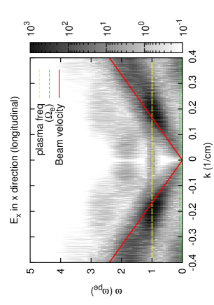
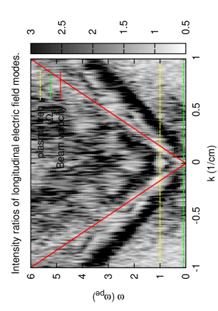
Figure 4: Left: Dispersion plot of the longitudinal electric field intensity along the beam direction. The beam resonance deposits large amounts of energy into the beam driven mode. Right: Increase (ratio) of electric field spectral energy between the weak beam and strong beam simulation.

The $k_{x}=0$ plane of $\vec{k}$-space was used to obtain the $k-\omega$ dispersion plot in Fig. 5 (left). In the plot, the electromagnetic mode is clearly visible as a parabola with cutoff at the plasma frequency. Additionally, lower velocity modes dominate the low $\omega$ values, probably mainly consisting of improperly resolved Alfvén waves (which are of no significance to the processes here).

Most importantly however, two horizontal bands in this plot are noticeable, localized at $\omega=\omega_{pe}$ and $2\omega_{pe}$ respectively. These bands do not follow the dispersion relations of any mode predicted by linear theory, which indicates that their origin is of non-linear nature. Kinematically, they correlate with the predicted three-wave interaction processes in Eq. 2 and 3 - assuming a coupling of waves of opposite-directed $k$-vectors from the resonantly excited longitudinal modes.

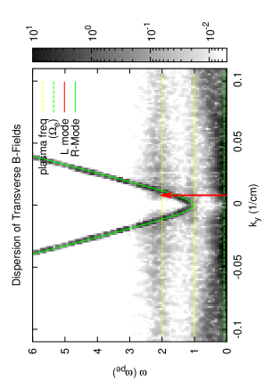
Figure 5: Left: Dispersion plot of the transverse magnetic field intensity (arb. units), with wave propagation direction perpendicular to the electron beam. Along the electromagnetic mode, resonances at $\omega_{pe}$ and $2\omega_{pe}$ are visible (dashed lines). The theoretically predicted point of interaction is denoted by the red arrow. Right: Ratio of intensities between the weak beam and strong beam simulations. Significant increase in energy is visible at the fundamental and harmonic frequency bands, especially at their upper edge.

The $k$-value of maximum coupling of the harmonic emission predicted by Eq. 8 is $k_{y}=8.3\cdot 10^{-3}\mathrm{cm}$, which matches the point of resonance visible in the simulation results (marked as a red arrow in Fig. 5). It is noteworthy that the intensities of the two bands are quite similar, in contrast to observations which typically show higher intensity in the harmonic than fundamental emission. This is, however, assumed to be a propagation effect: due to the close proximity of the emission to the plasma frequency, the local medium has a much higher index of refraction for the fundamental than the harmonic emission. The harmonic emission can hence escape the emission region much easier, and leads to a stronger signal in observations.

Apart from the plasma frequency and its harmonic, some intensity is also visible along the electromagnetic mode’s dispersion relation at other frequencies. This excitation stems from the inherent numerical noise of the particle in cell simulation, caused by the relatively low particle number per cell.

4 Conclusion

Using our fully relativistic particle-in-cell code ACRONYM, we have simulated electron beam driven wave excitation and subsequent wave couplings in a CME-foreshock environment. The complete spatial and temporal information obtainable from a numerical simulation provides improved insight into the wave processes in the emission region over satellite measurements: Analysis of resulting k-space wave distributions yields kinematically sound emission patterns, consistent with analytical predictions about the type II emission mechanism. Further analysis of spatial and temporal data provides evidence of nonlinear three-wave interaction between beam driven electrostatic modes to create electromagnetic modes at fundamental and harmonic frequencies with roughly equivalent intensities.

The fundamental and harmonic emission features visible in $k$-space representations of the simulated fields match those produced in Karlicky & Barta (2010). Since the emission in our runs was self-consistently produced from electron beams exciting Langmuir waves instead of artificial monochromatic excitation, these features are less strongly peaked, noisier and less pronounced, but otherwise share the emission characteristics.

4.1 Outlook

The beam intensity is just one of multiple tunable parameters of the emission process. Further parameters include beam velocity, background magnetic field intensity and the beam electrons’ pitch angle distribution. Simulations are currently underway, studying the behaviour of the system under variation of these parameters.

The enormous computational demands of particle-in-cell simulations are still a limiting factor, determining the maximum temporal extent of the runs. Slow wave interaction processes, like the scattering of Langmuir waves on sound waves (Eq. 1) are still insufficiently resolvable, and future improvements in computing power and kinetic plasma simulation techniques will be required to create complete, all-encompassing simulations of this emission mechanism.

An alternative simulation method worth studying would be a Vlasov code which, while equally or even more numerically challenging, would be able to simulate similar plasma behaviour free of effects due to statistical noise.

5 Acknowledgements

The simulations in this research have been made possible through computing grants by the Juelich Supercomputing Centre (JSC) and the CSC - IT Center for Science Ltd., Espoo, Finland.
UG acknowledges support by the Elite Network of Bavaria.
FS acknowledges support from the Deutsche Forschungsgemeinschaft through grant SP 1124/1
This work has been supported by the European Framework Programme 7 Grant Agreement SEPServer - 262773
We wish to express special thanks to our reviewer for his constructive and helpful comments.

References

- Aurass et al. (1994) Aurass, H., Klein, K.-L., & Mann, G. 1994, in ESA Special Publication, Vol. 373, Solar Dynamic Phenomena and Solar Wind Consequences, the Third SOHO Workshop, ed. J. J. Hunt, 95
- Cairns et al. (2003) Cairns, I., Knock, S., Robinson, P., & Kuncic, Z. 2003, Space Science Reviews, 107, 27
- Cane et al. (1987) Cane, H. V., Sheeley, J., & Howard, R. A. 1987, J. Geophys. Res., 92, 9869
- Ganse et al. (2011a) Ganse, U., Kilian, P., Vainio, R., & Spanier, F. 2011a, Submitted to Solar Physics
- Ganse et al. (2011b) Ganse, U., Spanier, F., & Vainio, R. 2011b, in IAU Symposium, Vol. 274, IAU Symposium, ed. A. Bonanno, E. de Gouveia Dal Pino, & A. G. Kosovichev, 470–472
- J. I. Sakai & M. Karlický (2008) J. I. Sakai, & M. Karlický. 2008, A&A, 478, L15
- Karlicky & Barta (2010) Karlicky, M., & Barta, M. 2010, Proceedings of the International Astronomical Union, 6, 252
- Karlický & Vandas (2007) Karlický, M., & Vandas, M. 2007, Planet. Space Sci., 55, 2336
- Kilian et al. (2012) Kilian, P., Burkart, T., & Spanier, F. 2012, in High Performance Computing in Science and Engineering ’11, ed. W. E. Nagel, D. B. Kröner, & M. M. Resch (Berlin Heidelberg: Springer), 5–13
- Knock et al. (2001) Knock, S. A., Cairns, I. H., Robinson, P. A., & Kuncic, Z. 2001, Journal of Geophysical Research, 106, 25041
- Melrose (1986) Melrose, D. B. 1986, Instabilities in Space and Laboratory Plasmas (Instabilities in Space and Laboratory Plasmas, by D. B. Melrose, pp. 288. ISBN 0521305411. Cambridge, UK: Cambridge University Press)
- Nelson & Melrose (1985) Nelson, G. J., & Melrose, D. B. 1985, Type II bursts (Cambridge University Press), 333–359
- Pulupa & Bale (2008) Pulupa, M., & Bale, S. D. 2008, Astrophysical Journal, 676, 1330
- Reiner et al. (1998) Reiner, M. J., Kaiser, M. L., Fainberg, J., & Stone, R. G. 1998, J. Geophys. Res., 103, 29651
- Schmidt & Gopalswamy (2008) Schmidt, J. M., & Gopalswamy, N. 2008, Journal of Geophysical Research, 113, A08104
- Spanier & Vainio (2009) Spanier, F., & Vainio, R. 2009, Advanced Science Letters, 2, 337
- Thejappa et al. (2012) Thejappa, G., MacDowall, R. J., & Bergamo, M. 2012, ApJ, 745, 187
- Wild & McCready (1950) Wild, J., & McCready, L. 1950, Australian Journal of Scientific Research, 3, 387
- Willes & Cairns (2000) Willes, A. J., & Cairns, I. H. 2000, Physics of Plasmas, 7, 3167
- Yu & Guangli (2008) Yu, H., & Guangli, H. 2008, Advances in Space Research, 41, 1202
- Zlotnik et al. (1998) Zlotnik, E. Y., Klassen, A., Klein, K.-L., Aurass, H., & Mann, G. 1998, A&A, 331, 1087