Shadow prices and well-posedness in the problem of optimal investment and consumption with transaction costs

Abstract.

We revisit the optimal investment and consumption model of Davis and Norman (1990) and Shreve and Soner (1994), following a shadow-price approach similar to that of Kallsen and Muhle-Karbe (2010). Making use of the completeness of the model without transaction costs, we reformulate and reduce the Hamilton-Jacobi-Bellman equation for this singular stochastic control problem to a non-standard free-boundary problem for a first-order ODE with an integral constraint. Having shown that the free boundary problem has a smooth solution, we use it to construct the solution of the original optimal investment/consumption problem in a self-contained manner and without any recourse to the dynamic programming principle. Furthermore, we provide an explicit characterization of model parameters for which the value function is finite.

1. Introduction

Ever since the seminal work of Merton (see [Mer69] and [Mer71]), the problem of dynamic optimal investment and consumption occupied a central role in mathematical finance and financial economics. Merton himself, together with many of the researchers that followed him, made the simplifying assumption of no market frictions: there are no transaction costs, borrowing and lending occur at the same interest rate, the assets can be bought and sold immediately in any quantity and at the same price (perfect liquidity), etc. Among those, transaction costs are (arguably) among the most important and (demonstrably) the most studied.

1.1. Existing work

The problem of optimal investment where transactions cost are present has received (and continues to receive) considerable attention. Following the early work of Constantinides and Magill [CM76], Davis and Norman [DN90] considered a risky asset driven by the geometric Brownian Motion for which proportional transactions costs are levied on each transaction. These authors formulated the optimal investment/consumption problem as a singular stochastic control problem, and approached it using the method of dynamic programming. Very early in the game it has been intuited, and later proved to varying degrees of rigor, that the optimal strategy has the following general form:

1. The investor should not trade at all as long as his/her holdings stay within the so-called “no-trade region” - a wedge around the Merton-proportion line.

2. Outside the “no-trade region’ , the investor should trade so as to reach the no-trading region as soon as possible, and, then, adjust the portfolio in a minimal way in order not to leave it ever after.

Such a strategy first appeared in [CM76] and was later made more precise in [DN90]. The analysis of [DN90] was subsequently complemented by that of Shreve and Soner [SS94] who removed various technical conditions, and clarified the key arguments using the technique of viscosity solutions. Still, even in [SS94], technical conditions needed to be imposed. Most notably, the analysis there assumes that the problem is well posed, i.e., that the value function is finite; no necessary and sufficient condition for this assumption, in terms of the parameters of the model, is given in [SS94]. In fact, to the best of our knowledge, the present paper provides the first such characterization.

More recently, Kallsen and Muhle Karbe [KMK10] approached the problem using the concept of a shadow price, first introduced by [JK95] and [LPS98]. Roughly speaking, the shadow-price approach amounts to comparing the problem with transaction costs to a family of similar problems, but without transaction costs, whose risky-asset prices lie between the bid and ask prices of the original model. The most unfavorable of these prices is expected to yield the same utility as the original problem where transaction costs are paid. As shown in [KMK10], this approach works quite well for the case of the logarithmic utility, which admits an explicit solution of the problem without transaction costs in a very general class of not-necessarily Markovian models. The fact that the logarithmic utility is the only member of the CRRA (power) family of utility functions with that property makes a direct extension of their techniques seem difficult to implement. Very recently, and in parallel with our work, partial results in this direction have been obtained by Herczegh and Prokaj [HP11] whose approach (and the intuition behind it) is based on the second-order nonlinear free-boundary HJB equation of [SS94], and applies only to a rather restrictive range of parameters.

1.2. Our contributions.

Our results apply to the model introduced [DN90] or [SS94], and deal with general power-utility functions and general values of the parameters. It is based on the shadow-price approach, but quite different in philosophy and execution from that of either [KMK10] or [HP11]. Our contributions can be divided into two groups:

Novel treatment and proofs of, as well as insights into the existing results. We provide a new and complete path to the solution to the optimal investment/consumption problem with transaction costs and power-type utilities. Our approach, based on the notion of the shadow price, is fully self-contained, does not rely on the dynamic programming principle and expresses all the features of the solution in terms of a solution to a single, constrained free-boundary problem for a one-dimensional first-order ODE. This way, it is able to distinguish between various parameter regimes which remained hidden under the more abstract approach of [DN90] and [SS94]. Interestingly, most of those regimes turn out to be “singular”, in the sense that our first-order ODE develops a singularity in the right-hand side. While we are able to treat them fully, those cases require a much more delicate and insightful analysis. The results of both [KMK10] and [HP11] apply only to the parameter regimes where no singularity is present.

New results. One of the advantages of our approach is that it allows us to give an explicit characterization of the set of model parameters for which the optimal investment and consumption problem with transaction costs is well posed. As already mentioned above, to the best of our knowledge, such a characterization is new, and not present in the literature.

Not only as another application, but also as an integral part of our proof, we furthermore prove that a shadow price exists whenever the problem is well-posed.

Finally, our techniques can be used to provide precise regularity information about all of the analytic ingredients, the value function being one of them. Somewhat surprisingly, we observe that in the singular case these are not always real-analytic, even when considered away from the free boundary.

1.3. The organization of the paper.

The set-up and the main results are presented in Section 2. In Section 3 we describe the intuition and some technical considerations leading to our non-standard free-boundary problem. In Section 4, we prove a verification-type result, i.e., show how to solve the singular control problem, assuming that a smooth-enough solution for the free-boundary equation is available. The proof of existence of such a smooth solution is the most involved part of the paper. In order to make our presentation easier to parse, we split this proof into two parts. Section 5 presents the main ideas of the proof, accompanied by graphical illustrations. The rigorous proofs follow in Section 6.

2. The Problem and the Main Results

2.1. The Market

We consider a model of a financial market in which the price process $\{S_{t}\}_{t\in[0,\infty)}$ of the risky asset (form simplicity called the “stock”) is given by

$$dS_{t}=S_{t}(\mu\,dt+\sigma\,dB_{t}),\ t\in[0,\infty)\text{ with }S_{0}>0.$$

Here, $B$ is a standard Brownian motion, and $\mu>0$ and $\sigma>0$ are constants - parameters of the model. The information structure is given by the natural saturated filtration generated by $B$. An economic agent starts with $\eta_{S}$ shares of the stock and $\eta_{B}$ units of an interestless bond and invests in the two securities dynamically. Transaction costs are not assumed away, and we model them as proportional to the size of the transaction. More precisely, they are determined by two constants $\underline{\lambda}\in(0,1)$ and $\overline{\lambda}>0$: one gets only $\underline{S}_{t}=(1-\underline{\lambda})S_{t}$ for one share of the stock, but pays $\overline{S}_{t}=(1+\overline{\lambda})S_{t}$ for it.

2.2. Solvency and Admissible Strategies

We assume that the agent’s initial position $(\eta_{B},\eta_{S})$ is strictly solvent, which means that it can be liquidated to a positive cash position. More precisely, we assume that $\operatorname{Liq}(\eta_{B},\eta_{S},\underline{S}_{0},\overline{S}_{0})>0$ where

$$\operatorname{Liq}(\varphi^{0},\varphi,\underline{s},\overline{s})=\varphi^{0}+\varphi^{+}\underline{s}-\varphi^{-}\overline{s}.$$ (2.1)

The agent’s (consumption/trading) strategy is described by a triple $(\varphi^{0},\varphi,c)$ of optional processes such that $\varphi$ and $\varphi^{0}$ are right-continuous and of finite variation and $c$ is nonnegative and locally integrable, a.s. The processes $\varphi^{0}$ and $\varphi$ have the meaning of the amount of cash held in the money market and the number of shares in the risky asset, respectively, while $c$ is the consumption rate.

In order to incorporate the potential initial jump we distinguish between the initial values $(\varphi^{0}_{0-},\varphi_{0-})$ and the values $(\varphi^{0}_{0},\varphi_{0})$ (after which the processes are right-continuous). This is quite typical for optimal investment/consumption strategies, both in frictional and frictionless markets, when the agent initially holds stocks, in addition to bonds. In this spirit, we always assume that $(\varphi^{0}_{0-},\varphi_{0-})=(\eta_{B},\eta_{S}).$

A strategy $(\varphi^{0},\varphi,c)$ is said to be self-financing if

$$\begin{split}\varphi^{0}_{t}=\varphi^{0}_{0-}-\int_{0}^{t}\overline{S}_{u}d\varphi^{\uparrow}_{u}+\int_{0}^{t}\underline{S}_{u}d\varphi^{\downarrow}_{u}-\int_{0}^{t}c_{u}\,du,\end{split}$$ (2.2)

where $\varphi=\varphi_{0-}+\varphi^{\uparrow}-\varphi^{\downarrow}$ is the pathwise minimal (Hahn-Jordan) decomposition of $\varphi$ into a difference of two non-decreasing adapted, right-continuous processes, with possible jumps at time zero, as we assume that $\varphi^{\uparrow}_{0-}=\varphi^{\downarrow}_{0-}=0.$

The integrals used in (2.2) above, with respect to the (pathwise Stieltjes) measures $d\varphi^{\uparrow}$ and $d\varphi^{\downarrow}$ characterized by $d\varphi^{\uparrow}((a,b])=\varphi^{\uparrow}(b)-\varphi^{\uparrow}(a)$, and $d\varphi^{\downarrow}((a,b])=\varphi^{\downarrow}(b)-\varphi^{\downarrow}(a)$, for $0\leq a<b<\infty$ together with $d\varphi^{\uparrow}(\{0\})=\varphi^{\uparrow}(0)-\varphi^{\uparrow}(0-)=\varphi^{\uparrow}(0)$, and $d\varphi^{\downarrow}(\{0\})=\varphi^{\downarrow}(0)-\varphi^{\downarrow}(0-)=\varphi^{\downarrow}(0)$.

A self-financing strategy $(\varphi^{0},\varphi,c)$ is called admissible if its position is always solvent, i.e., if

$$\begin{split}\operatorname{Liq}(\varphi^{0}_{t},\varphi_{t},\underline{S}_{t},\overline{S}_{t})\geq 0,\text{ for all $t$, a.s. }\end{split}$$ (2.3)

The set of all admissible strategies with $\varphi^{0}_{0-}=\eta_{B}$ and $\varphi_{0-}=\eta_{S}$ is denoted by ${\mathcal{A}}$, and the set of all $c$ such that $(\varphi^{0},\varphi,c)\in{\mathcal{A}}$ for some $\varphi^{0}$ and $\varphi$ - the so-called financeable consumption processes - is denoted by ${\mathcal{C}}$.

2.3. Utility functions

For $p\in(-\infty,1)$, we consider the utility function $U:[0,\infty)\to[-\infty,\infty)$ of the power (CRRA) type. It is defined for $c\geq 0$ by

$$U(c)=\begin{cases}\tfrac{1}{p}c^{p},&c\neq 0,p\neq 0\\ \log(c),&c\neq 0,p=0,\end{cases}\text{ and }\ U(0)=\begin{cases}0,&p>0,\\ -\infty,&p\leq 0\end{cases}$$

Our task is to analyze the optimal investment and consumption problem, with the value

$$\begin{split}u=\sup_{c\in{\mathcal{C}}}{\mathcal{U}}(c),\text{ where }\ {\mathcal{U}}(c)={\mathbb{E}}\left[\int_{0}^{\infty}e^{-\delta t}U(c_{t})\,dt\right],\end{split}$$ (2.4)

and $\delta>0$ stands for the (constant) impatience rate. As part of the definition of ${\mathcal{U}}$, we posit that ${\mathcal{U}}(c)=-\infty$ unless ${\mathbb{E}}\left[\int_{0}^{\infty}e^{-\delta t}(U(c_{t}))^{-}\,dt\right]<\infty$.

2.4. Consistent price processes

An Itô-process ${\tilde{S}}$ is called a consistent price (process) if $\underline{S}_{t}\leq{\tilde{S}}_{t}\leq\overline{S}_{t}$, for all $t\geq 0$, a.s.; the set of all consistent prices is denoted by ${\mathcal{S}}$. For each consistent price ${\tilde{S}}\in{\mathcal{S}}$, and a solvent pair of initial holdings $(\eta_{B},\eta_{S})\in{\mathbb{R}}^{2}$ such that $\operatorname{Liq}(\eta_{B},\eta_{S},\underline{S}_{0},\overline{S}_{0})\geq 0$, we define the set ${\mathcal{A}}({\tilde{S}})$ of (frictionless) admissible strategies $(\varphi^{0},\varphi,c)$, as we would in the standard frictionless market where the price-process is given by ${\tilde{S}}$. More precisely, for $(\varphi^{0},\varphi,c)$ to belong to ${\mathcal{A}}({\tilde{S}})$ it is necessary and sufficient that the following three conditions hold

1. $\varphi^{0},\varphi$ and $c$ are progressively measurable, $c_{t}\geq 0$, a.s., for all $t\in[0,\infty]$,

2. $\varphi^{0}_{0-}=\eta_{B}$ and $\varphi_{0-}=\eta_{S}$, and

3. $V_{t}=\varphi^{0}_{t}+\varphi_{t}{\tilde{S}}_{t}\geq 0$, for all $t\in[0,\infty)$, a.s,. and

   $$\begin{split}V_{t}=V_{0-}+\int_{0}^{t}\varphi_{u}\,d{\tilde{S}}_{u}-\int_{0}^{t}c_{u}\,du,t\geq 0,\text{ a.s.}\end{split}$$ (2.5)

The set of processes $\{c_{t}\}_{t\in[0,\infty)}$ that appear as the third component of an element of ${\mathcal{A}}({\tilde{S}})$ will be denoted by ${\mathcal{C}}({\tilde{S}})$, i.e.,

$${\mathcal{C}}({\tilde{S}})=\{c\,:\,\text{there exist }\varphi^{0},\varphi,\text{ such that }(\varphi^{0},\varphi,c)\in{\mathcal{A}}({\tilde{S}})\}.$$

The elements of ${\mathcal{C}}({\tilde{S}})$ can be interpreted as the consumption processes financeable from the initial holding $(\eta_{B},\eta_{S})$ in the frictionless market modeled by ${\tilde{S}}$. The intuition that the presence of transaction costs can only reduce the collection of financeable consumption processes can be formalized as in the following easy proposition.

Proposition 2.1.

${\mathcal{C}}\subseteq{\mathcal{C}}({\tilde{S}})$, for each ${\tilde{S}}\in{\mathcal{S}}$.

Proof.

For $c\in{\mathcal{C}}$, let $(\varphi^{0},\varphi)$ be such that $(\varphi^{0},\varphi,c)\in{\mathcal{A}}$. By the self-financing condition (2.2), the fact that $\underline{S}_{t}\leq{\tilde{S}}_{t}\leq\overline{S}_{t}$ and integration by parts (simplified by the fact that ${\tilde{S}}$ is continuous), we have

$$\begin{split}-\int_{0}^{t}c_{u}\,du&=\varphi^{0}_{t}-\varphi^{0}_{0-}+\int_{0}^{t}\overline{S}_{u}d\varphi^{\uparrow}_{u}-\int_{0}^{t}\underline{S}_{u}d\varphi^{\downarrow}_{u}\geq\varphi^{0}_{t}-\varphi^{0}_{0-}+\int_{0}^{t}{\tilde{S}}_{u}\,d\varphi_{u}\\ &=\varphi^{0}_{t}-\varphi^{0}_{0-}+{\tilde{S}}_{t}\varphi_{t}-{\tilde{S}}_{0}\varphi_{0-}-\int_{0}^{t}\varphi_{u}\,d{\tilde{S}}_{u}\end{split}$$ (2.6)

Therefore, by the admissibility criterion (2.3), we have

$$\begin{split}\eta_{B}+{\tilde{S}}_{0}\eta_{S}+\int_{0}^{t}\varphi_{u}\,d{\tilde{S}}_{u}-\int_{0}^{t}c_{u}\,du\geq\varphi^{0}_{t}+{\tilde{S}}_{t}\varphi_{t}\geq 0.\end{split}$$ (2.7)

It remains to set $\tilde{\varphi}=\varphi$ and $\tilde{\varphi}^{0}_{t}=\eta_{B}+\int_{0}^{t}\tilde{\varphi}_{u}\,d{\tilde{S}}_{u}-\int_{0}^{t}c_{u}\,du-\tilde{\varphi}_{t}\tilde{S}_{t}+\eta_{S}\tilde{S}_{0}$, and observe that (2.7) directly implies (2.5). Thus, $(\tilde{\varphi}^{0},\tilde{\varphi},c)\in{\mathcal{A}}({\tilde{S}})$. ∎

It will be important in the sequel to be able to check whether an element of ${\mathcal{C}}({\tilde{S}})$ belongs to ${\mathcal{C}}$. It happens, essentially, when a strategy that finances it “buys” only when ${\tilde{S}}_{t}=\overline{S}_{t}$ and “sells” only when ${\tilde{S}}_{t}=\underline{S}_{t}$. A precise statement is given in the following proposition.

Proposition 2.2.

Given ${\tilde{S}}\in{\mathcal{S}}$, let $c\in{\mathcal{C}}({\tilde{S}})$ be such that there exist processes $\varphi^{0}$ and $\varphi$ such that

1. $(\varphi^{0},\varphi,c)\in{\mathcal{A}}({\tilde{S}})$,

2. $\varphi$ is a right-continuous process of finite variation, and

3. the Stieltjes measure on $[0,\infty)$ induced by $\varphi^{\uparrow}$ is carried by $\{{\tilde{S}}_{t}=\overline{S}_{t}\}$ and that induced by $\varphi^{\downarrow}$ by $\{{\tilde{S}}_{t}=\underline{S}_{t}\}$.

Then, $c\in{\mathcal{C}}$.

Proof.

Let the triplet $(\varphi^{0},\varphi,c)\in{\mathcal{A}}({\tilde{S}})$ satisfy the conditions of the proposition. In particular, we have

$$\begin{split}0&=\eta_{B}+\eta_{S}{\tilde{S}}_{0}-\varphi^{0}_{t}-\varphi_{t}{\tilde{S}}_{t}+\int_{0}^{t}\varphi_{u}\,d{\tilde{S}}_{u}-\int_{0}^{t}\,c_{u}\,du.\end{split}$$

Thanks to condition (3), the integration-by-parts formula and the self-financing property (2.2), it follows that

$$\begin{split}\varphi^{0}_{t}&=\eta_{B}-\int_{0}^{t}{\tilde{S}}_{t}\,d\varphi_{u}-\int_{0}^{t}\,c_{u}\,du=\eta_{B}-\int_{0}^{t}{\tilde{S}}_{t}\,d\varphi^{\uparrow}_{u}+\int_{0}^{t}{\tilde{S}}_{t}\,d\varphi^{\downarrow}_{u}-\int_{0}^{t}c_{u}\,du\\ &=\eta_{B}-\int_{0}^{t}\overline{S}_{t}\,d\varphi^{\uparrow}_{u}+\int_{0}^{t}\underline{S}_{t}\,d\varphi^{\downarrow}_{u}-\int_{0}^{t}c_{u}\,du.\end{split}$$

Hence, $c\in{\mathcal{C}}$. ∎

2.5. Shadow Problems

For each consistent price process ${\tilde{S}}$, we define an auxiliary optimal-consumption problem - called the ${\tilde{S}}$-problem, with the value $u({\tilde{S}})$, by

$$\begin{split}u({\tilde{S}})=\sup_{c\in{\mathcal{C}}({\tilde{S}})}{\mathcal{U}}(c),\text{ so that }u\leq\inf_{{\tilde{S}}\in{\mathcal{S}}}u({\tilde{S}}),\end{split}$$ (2.8)

where $u$ is defined as in (2.4), and the inequality on the right is implied by Proposition 2.1. In words, each consistent price ${\tilde{S}}$ affords at least as good an investment opportunity as the original frictional market.

It is in the heart of our approach to show that the duality gap, in fact, closes, i.e., that the inequality in (2.8) becomes an equality; the worst-case shadow problem performs no better than frictional one.

Definition 2.3.

A consistent price ${\tilde{S}}$ is called a shadow price if $u=u({\tilde{S}})$.

The central idea of the present paper is to look for a shadow price as the minimizer of the right-hand side of (2.8) viewed as a stochastic control problem. More precisely, we turn our attention to a search for an optimizer in the shadow problem:

$$\begin{split}{\tilde{u}}=\inf_{{\tilde{S}}\in{\mathcal{S}}}u({\tilde{S}}).\end{split}$$ (2.9)

We start by tackling the shadow problem in a formal manner and deriving an analytic object (a free-boundary problem) related to its solution. Next, we show that this free-boundary problem indeed admits a solution and use it to construct the candidate shadow price. Finally, instead of showing that our candidate is indeed an optimizer for (2.9) and that $u={\tilde{u}}$, we use the following direct consequence of Proposition 2.2.

Proposition 2.4.

Suppose that for ${\tilde{S}}\in{\mathcal{S}}$ there exists a triplet $(\varphi^{0},\varphi,c)$ such that

1. $(\varphi^{0},\varphi,c)$ satisfies conditions (1), (2) and (3) of Proposition 2.2, and

2. ${\mathcal{U}}(c^{\prime})\leq{\mathcal{U}}(c)$, for all $c^{\prime}\in{\mathcal{C}}({\tilde{S}})$,

Then, ${\tilde{S}}$ is a shadow price.

Remark 2.5.

The route we take towards the existence of a shadow price may appear to be somewhat circuitous. It is chosen so as to maximize the intuitive appeal of the method and minimize (already formidable) technical difficulties.

While the remainder of the paper is devoted to the implementation of the above idea, we anticipate its final results here, for the convenience of the reader. An important by-product of our analysis is the explicit characterization of those parameter values which result in a well-posed problem (the value function is finite). To the best of our knowledge, such a characterization is not present in the literature, and the finiteness of the value function is either assumed (as in [SS94]) or deduced from rather strong conditions (as in [KMK10]).

Theorem 2.6.

Given the environment parameters $\mu,\sigma\in(0,\infty)$ and the transaction costs $\underline{\lambda}\in(0,1)$, $\overline{\lambda}>0$, the following statements are equivalent:

(1) The problem is well posed, i.e

$$-\infty<u<\infty,$$

whenever $\operatorname{Liq}(\eta_{B},\eta_{S},\underline{S}_{0},\overline{S}_{0})>0$.

(2) The parameters of the model satisfy one of the following three conditions:
- $p\leq 0$,
- $0<p<1$ and $\mu<\sqrt{\frac{2\delta(1-p)\sigma^{2}}{p}}$,
- $0<p<1$, $\sqrt{\frac{2\delta(1-p)\sigma^{2}}{p}}\leq\mu<\frac{\delta}{p}+\frac{(1-p)\sigma^{2}}{2}$ and

$$C(\mu,\sigma,p,\delta)<\log(\tfrac{1+\overline{\lambda}}{1-\underline{\lambda}}),$$

where the function $C(\cdot,\cdot,\cdot,\cdot)$ is given by (6.8) in a closed form.

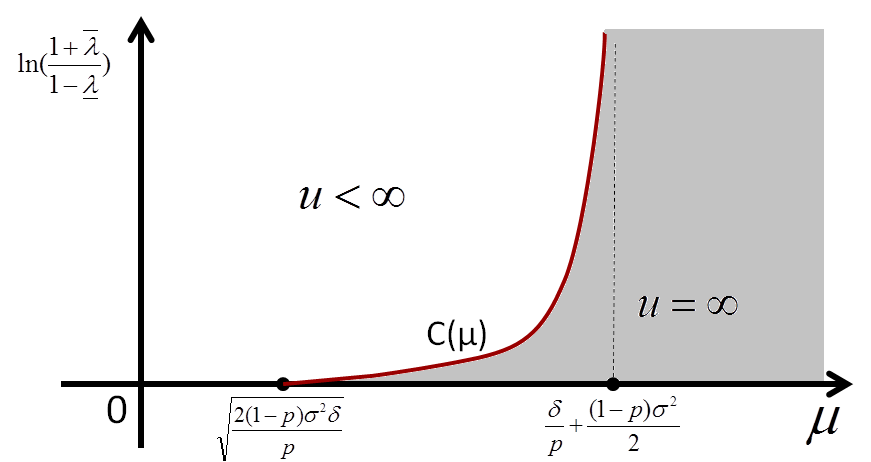
Figure 1. The well-posedness region.

Remark 2.7.

For $\sigma=0$, the third condition in (2) above reduces to a well-known condition of Shreve and Soner. Indeed, the entire Section 12 in [SS94], culminating in Theorem 12.2, p. 677, is devoted to the well-posedness problem with two bonds (i.e, with $\sigma=0$).

As demonstrated by our second main result, the shadow-price approach not only allows us to fully characterize the conditions under which a solution to the frictional optimal investment/consumption problem exists, but it also sheds light on its form and regularity.

Theorem 2.8.

Given the parameters $\mu,\sigma\in(0,\infty)$ and the transaction costs $\underline{\lambda}\in(0,1)$, $\overline{\lambda}>0$, we assume that well-posedness conditions of Theorem 2.6 hold. Then

1. There exist constants $\underline{x},\overline{x}$ with $0<\underline{x}<\overline{x}$ and a function $g\in C^{2}[\underline{x},\overline{x}]$ such that

   1. $g^{\prime}(x)>0$ for $x\in(\underline{x},\overline{x})$, and $g$ satisfies the equation

      $$\begin{split}\inf_{\Sigma,\theta\in{\mathbb{R}}}\Big{(}\tfrac{1}{2}\Sigma^{2}\tfrac{x}{g^{\prime}(x)}-\alpha_{q}(\Sigma,\theta)x-\beta(\theta)g(x)+\gamma(\theta)\Big{)}=0,\ x\in(\underline{x},\overline{x}),\end{split}$$ (2.10)

      where

      $$\begin{split}&q=\tfrac{p}{1-p},\ \alpha_{q}(\Sigma,\theta)=\theta\sigma-\mu-\Sigma\Big{(}\tfrac{1}{2}\Sigma+\sigma-\theta(1+q)\Big{)},\\ &\beta(\theta)=(1+q)\Big{(}\delta-\tfrac{1}{2}q\theta^{2}\Big{)},\text{ and }\gamma(\theta)=\begin{cases}\tfrac{1}{2}\theta^{2},&p=0,\\ \operatorname{sgn}(p),&p\neq 0.\end{cases}\end{split}$$ (2.11)

   2. the following boundary/integral conditions are satisfied:

      $$\begin{split}g^{\prime}(\underline{x}+)=g^{\prime}(\overline{x}-)=0\text{ and }\int_{\underline{x}}^{\overline{x}}\tfrac{g^{\prime}(x)}{x}\,dx=\log(\tfrac{1+\overline{\lambda}}{1-\underline{\lambda}}).\end{split}$$ (2.12)

   3. The function $h:[\underline{x},\overline{x}]\to{\mathbb{R}}$, defined by

      $$\begin{split}h(x)=\begin{cases}(1-x)g^{\prime}(x)+1,&p=0,\\ qg(x)\left(g^{\prime}(x)+1\right)-(q+1)xg^{\prime}(x),&p\neq 0,\\ \end{cases}\end{split}$$ (2.13)

      admits no zeros on $[\underline{x},\overline{x}]$.

2. For any $(\eta_{B},\eta_{S})$ such that

   $$\operatorname{Liq}(\eta_{B},\eta_{S},\underline{S}_{0},\overline{S}_{0})>0,$$ (2.14)

   there exists a shadow price $\{{\tilde{S}}_{t}\}_{t\in[0,\infty)}$, of the form ${\tilde{S}}_{t}=S_{t}e^{f(X^{{\hat{x}}}_{t})}$, where

   • $f(x)=\underline{y}+\int_{x}^{\overline{x}}\tfrac{g^{\prime}(t)}{t}\,dt$, for $x\in[\underline{x},\overline{x}]$,

   • the value of the constant ${\hat{x}}$ is determined as in Proposition 4.5, and

   • $X^{{\hat{x}}}$ is the unique solution of reflected SDE (4.3) with $X^{{\hat{x}}}_{0}={\hat{x}}$.

3. For any $(\eta_{B},\eta_{S})$ satisfying (2.14), the value $u$ and an optimal investment/consumption strategy $(\hat{\varphi}^{0},\hat{\varphi},{\hat{c}})$ for the main problem (2.4) are given by

   $$u={\hat{u}}(\eta_{B},\eta_{S};{\hat{x}}),\quad(\hat{\varphi}^{0}_{t},\hat{\varphi}_{t},{\hat{c}}_{t})=(\hat{\varphi}_{t}^{0,{\hat{x}}},\hat{\varphi}_{t}^{{\hat{x}}},{\hat{c}}_{t}^{{\hat{x}}}),$$

   where ${\hat{x}}$ is defined in Proposition 4.5, and ${\hat{u}},\hat{\varphi}_{t}^{0,x},\hat{\varphi}_{t}^{x}$ and ${\hat{c}}_{t}^{x}$ in Lemma 4.4.

Remark 2.9.

In (2.12), if $(\underline{x},g(\underline{x}))=P$ ($P$ is a singular point described in Section 5), then the condition $g^{\prime}(\underline{x})=0$ can be violated. For this exceptional case, Proposition 4.2 is still valid: More precisely, in the part (2) of Proposition 4.2, we need to show that $\frac{g^{\prime}(X_{t}^{x})}{X_{t}^{x}}d\Phi_{t}^{x}\equiv 0$. If $(\underline{x},g(\underline{x}))=P$, in (4.3), the drift is positive and the volatility is zero, thus, we conclude that $d\Phi_{t}^{x\uparrow}\equiv 0$.

3. A heuristic derivation of a free-boundary problem

The purpose of the present section is to provide a heuristic derivation of a free-boundary problem for a one-dimensional first-order ODE which will later be used to construct a shadow process and the solution of our main problem. With the fully rigorous verification coming later, we often do not pay attention to integrability or measurability conditions and formally push through many steps in this section.

We start by splitting the shadow problem (2.9) according to the starting value of the process ${\tilde{S}}$:

$$\begin{split}{\tilde{u}}=\inf_{s_{0}\in[(1-\underline{\lambda})S_{0},(1+\overline{\lambda})S_{0}]}\quad\inf_{{\tilde{S}}\in{\mathcal{S}},{\tilde{S}}_{0}=s_{0}}\quad\sup_{c\in{\mathcal{C}}({\tilde{S}})}{\mathcal{U}}(c).\end{split}$$ (3.1)

One can significantly simplify the analysis of the above problem by noting that, since each ${\tilde{S}}$ is a strictly positive Itô-process, we can always choose processes $\Sigma=\Sigma({\tilde{S}})$ and $\theta=\theta({\tilde{S}})$ such that

$$d{\tilde{S}}_{t}={\tilde{S}}_{t}(\sigma+\Sigma_{t})\,(dB_{t}+\theta_{t}\,dt),\ {\tilde{S}}_{0}=s_{0}.$$

It pays to pass to the logarithmic scale, and introduce the process $Y_{t}=\log({\tilde{S}}_{t}/S_{t})$, whose dynamics is given by

$$\begin{split}dY_{t}=\alpha_{0}(\theta_{t},\Sigma_{t})\,dt+\Sigma_{t}\,dB_{t},\end{split}$$ (3.2)

on the natural domain $Y_{t}\in[\underline{y},\overline{y}]$. Here, $\underline{y}=\log(1-\underline{\lambda})$, $\overline{y}=\log(1+\overline{\lambda})$ and the function $\alpha_{0}$ is given by (2.11) for $q=0$. This way, the family of consistent price processes is parametrized by the set

$${\mathcal{P}}=\{(y,\Sigma,\theta)\,:\,y\in[\underline{y},\overline{y}],(\Sigma,\theta)\in{\mathcal{P}}(y)\},$$

where ${\mathcal{P}}(y)$ is the set of all pairs of regular-enough processes $(\Sigma,\theta)$ such that the process $\{Y_{t}\}_{t\in[0,\infty)}$, given by (3.2) and starting at $Y_{0}=y$, stays in the interval $[\underline{y},\overline{y}]$, a.s.

We note that the market modeled by ${\tilde{S}}$ is complete, and that, thanks to the absence of friction, the agent with the initial holdings $(\eta_{B},\eta_{S})$ will achieve the same utility as the one who immediately liquidates the position, i.e., the one with the initial wealth of $\eta_{B}+S_{0}e^{y}\eta_{S}$. Therefore, the standard duality theory suggests that

$$\begin{split}\sup_{c\in{\mathcal{C}}({\tilde{S}})}{\mathcal{U}}(c)=\inf_{z>0}\Big{(}(\eta_{B}+S_{0}e^{y}\eta_{S})z+{\mathcal{V}}(z{\mathcal{E}}(-\theta\cdot B))\Big{)},\end{split}$$ (3.3)

where ${\tilde{S}}$ and $(y,\Sigma,\theta)$ are related as above and

$$\begin{split}V(z)=\sup_{c>0}(U(c)-cz),\quad{\mathcal{V}}(Z)={\mathbb{E}}\left[\int_{0}^{\infty}e^{-\delta t}V(e^{\delta t}Z_{t})\,dt\right].\end{split}$$ (3.4)

Remark 3.1.

The Legendre-Fenchel transform $V$ of $U$ admits an explicit and simple expression in the case of a power utility. Indeed, we have

$$V(z)=\begin{cases}\tfrac{1}{q}z^{-q},&p\neq 0,\\ -1-\log(z),&p=0,\end{cases}$$

where $q=p/(1-p)$. The parameter $q$ is the negative of the conjugate exponent of $p$, i.e., $\tfrac{1}{p}-\tfrac{1}{q}=1$ ($q=0$, for $p=0$) and this relationship will be assumed to hold throughout the paper without explicit mention.

Consequently, if we combine (3.1) and (3.3), we obtain the following equality:

$$\begin{split}{\tilde{u}}=\inf_{(y,z)\in[\underline{y},\overline{y}]\times(0,\infty)}\Big{(}(\eta_{B}+S_{0}e^{y}\eta_{S})z+\inf_{(\Sigma,\theta)\in{\mathcal{P}}(y)}{\mathcal{V}}(z{\mathcal{E}}(-\theta\cdot B))\Big{)}.\end{split}$$ (3.5)

The expression above is particularly convenient because it separates the shadow problem into a stochastic control problem over ${\mathcal{P}}(y)$, and a (finite-dimensional) optimization problem over $y$ and $z$, which can be solved separately.

3.1. A dimensional reduction

Thanks to homogeneity ($\log$-homogeneity for $p=0$) of the map $z\mapsto{\mathcal{V}}(zZ)$, a dimensional reduction is possible in the inner control problem in (3.5). Indeed, with $\hat{\delta}=\delta(1+q)$, we have

$${\mathcal{V}}(z{\mathcal{E}}(-\theta\cdot B))=\begin{cases}-\tfrac{2+\log(z)}{\delta}+{\mathbb{E}}\left[\int_{0}^{\infty}e^{-\delta t}\Big{(}-\log({\mathcal{E}}(-\theta\cdot B)_{t})\Big{)}\,dt\right],&p=0,\\ \tfrac{z^{-q}}{q}\,{\mathbb{E}}\left[\int_{0}^{\infty}e^{-\hat{\delta}t}{\mathcal{E}}(-\theta\cdot B)_{t}^{-q}\,dt\right],&p\neq 0.\\ \end{cases}$$

Hence,

$$\begin{split}{\tilde{u}}=\inf_{y\in[\underline{y},\overline{y}]}\begin{cases}\tfrac{1}{\delta}\Big{(}-1+\log\Big{(}\delta(\eta_{B}+S_{0}e^{y}\eta_{S})\Big{)}+w(y)\Big{)},&p=0\\ \tfrac{(\eta_{B}+S_{0}e^{y}\eta_{S})^{p}}{p}\left|w(y)\right|^{1-p},&p\neq 0,\end{cases}\end{split}$$ (3.6)

where

$$w(y)=\inf_{(\Sigma,\theta)\in{\mathcal{P}}(y)}\begin{cases}{\mathbb{E}}\left[\int_{0}^{\infty}\delta e^{-\delta t}\Big{(}-\log({\mathcal{E}}(-\theta\cdot B)_{t})\Big{)}\,dt\right],&p=0,\\ \operatorname{sgn}(p){\mathbb{E}}\left[\int_{0}^{\infty}e^{-\hat{\delta}t}{\mathcal{E}}(-\theta\cdot B)_{t}^{-q}\,dt\right],&p\neq 0.\end{cases}$$

In the heuristic spirit of the present section, it will be assumed that the processes of the form $\theta\cdot B$ and ${\mathcal{E}}(q\theta\cdot B)$ are (true) martingales so that the definition of the stochastic exponential and the simple identity

$$\begin{split}{\mathcal{E}}(-\theta\cdot B)^{-q}={\mathcal{E}}(q\theta\cdot B)\exp\Big{(}\tfrac{1}{2}q(1+q)\int_{0}^{\cdot}\theta_{u}^{2}\,du\Big{)}\end{split}$$ (3.7)

can be used to simplify the expression for $w$ even further:

$$\begin{split}w(y)=\inf_{(\Sigma,\theta)\in{\mathcal{P}}(y)}\begin{cases}\tfrac{1}{2}{\mathbb{E}}\left[\int_{0}^{\infty}e^{-\delta t}\theta^{2}_{t}\,dt\right],&p=0,\\ \operatorname{sgn}(p){\mathbb{E}}^{\bar{{\mathbb{P}}}}\left[\int_{0}^{\infty}e^{-\hat{\delta}t}e^{\tfrac{1}{2}q(1+q)\int_{0}^{t}\theta^{2}_{u}\,du}\,dt\right],&p\neq 0.\end{cases}\end{split}$$ (3.8)

Here, the measure $\bar{{\mathbb{P}}}$ is (locally) given by $d\bar{{\mathbb{P}}}={\mathcal{E}}(q\theta\cdot B)\,d{\mathbb{P}}$. By Girsanov’s theorem the process

$$\begin{split}\bar{B}=B-\int_{0}^{\cdot}q\theta_{u}\,du\end{split}$$ (3.9)

is (locally) a $\bar{{\mathbb{P}}}$-Brownian motion and the dynamics of the process $Y$ can be conveniently written as

$$dY_{t}=\alpha_{q}(\theta_{t},\Sigma_{t})\,dt+\Sigma_{t}\,d\bar{B}_{t}.$$

The expression inside the infimum in (3.8) involves a discounted running cost. Hence, it fits in the classical framework of optimal stochastic control, and a formal HJB-equation can be written down. We note that even though the process ${\mathcal{E}}(-\theta\cdot B)$ appears in the original expression for $w$, the simplification in (3.8) allows us to drop it from the list of state variables and, thus, reduce the dimensionality of the problem. Indeed, the formal HJB has the following form:

$$\begin{split}\inf_{\Sigma,\theta}\Big{(}\tfrac{1}{2}\Sigma^{2}w^{\prime\prime}(y)+\alpha_{q}(\Sigma,\theta)w^{\prime}(y)-\beta(\theta)w(y)+\gamma(\theta)\Big{)}=0,\ y\in(\underline{y},\overline{y})\end{split}$$ (3.10)

where the functions $\beta$ and $\gamma$ are defined in (2.11).

In order to fully characterize the optimization problem, we need to impose the boundary conditions at $\underline{y}$ and $\overline{y}$ to enforce the requirement that $Y$ stay within the interval $[\underline{y},\overline{y}]$. These amount to turning off the diffusion completely and leaving only the drift in the appropriate (inward) direction when $Y$ reaches the boundary. Thanks to the form of the function $\alpha_{q}$ and the equation (3.10), as well as the expectation that $w^{\prime}$ be bounded on $[\underline{y},\overline{y}]$, we are led to the boundary condition

$$\begin{split}w^{\prime\prime}(\underline{y})=w^{\prime\prime}(\overline{y})=+\infty.\end{split}$$ (3.11)

It will be shown in the following section that, in addition to the annihilation of the diffusion coefficient, (3.11) will ensure that the drift coefficient $\alpha_{q}$ will indeed have the proper sign of at the boundary.

3.2. Shadow price as a strategy in a game

By interpreting the problem of shadow prices as a game, one can arrive to the two-point boundary problem (3.10), (3.11) without the use of duality.

Let $\xi(y)=\eta_{B}+\eta_{S}S_{0}e^{y}$ denote the initial wealth of the investor who is not subject to transaction costs, for a fixed $\eta_{B},\eta_{S}$ and $y\in[\overline{y},\underline{y}]$. Finding a shadow price now amounts to the following:

1. given $(\theta,\Sigma)$, solving the optimal investment problem for an investor with initial wealth $\xi(y)$ i.e., maximizing the expected discounted utility

   $${\mathbb{E}}[\int_{0}^{\infty}e^{-\delta t}U(c_{t})].$$

   over $(\varphi,c)$ (numbers of shares of ${\tilde{S}}$ and the rate of consumption).

2. minimizing the obtained value over $(\theta,\Sigma)$, and

3. finally, further minimizing over $y\in[\overline{y},\underline{y}].$

Up to the last minimization over $y$, the above defines a stochastic game with the value

$$v(\xi,y):=\inf_{\theta,\Sigma}\sup_{\pi,c}{\mathbb{E}}[\int_{0}^{\infty}e^{-\delta t}U(c_{t})].$$

The corresponding Isaacs equation with a two dimensional state $(\Xi,Y)$ and the initial condition $(\Xi_{0},Y_{0})=(\xi,y)$ scales as

$$v(\xi,y)=\frac{\xi^{p}}{p}|w(y)|^{1-p}\text{ (compare to \eqref{equ:hfu-form}).}$$

Consequently, it can be reduced to a one-dimensional equation for $w(y)$, with $y\in[\overline{y},\underline{y}]$, which turns out to be exactly the boundary-value problem (3.10), (3.11). Once the game is solved, we can find a shadow price by simply minimizing the value $v(\xi(y),y)$ over $y\in[\overline{y},\underline{y}]$.

We believe that a similar approach - namely of rewriting the problem of optimal investment and consumption with transaction costs as a game, through the use of consistent prices - works well in more general situations, e.g., when multiple assets are present.

3.3. An order reduction

Finally, based on the fact that the equation (2.10) is autonomous, we introduce an order-reducing change of variable. With $w^{\prime}$ expected to be increasing and continuous on $[\underline{y},\overline{y}]$, we define the function $g:[\underline{x},\overline{x}]\to{\mathbb{R}}$, with $\overline{x}=-w^{\prime}(\underline{y})$ and $\underline{x}=-w^{\prime}(\overline{y})$ by $w(y)=g(-w^{\prime}(y))$. This transforms the equation (2.10) into

$$\begin{split}\inf_{\Sigma,\theta}\Big{(}\tfrac{1}{2}\Sigma^{2}\tfrac{x}{g^{\prime}(x)}-\alpha_{q}(\Sigma,\theta)x-\beta(\theta)g(x)+\gamma(\theta)\Big{)}=0,\end{split}$$

with (free) boundary conditions $g^{\prime}(\underline{x})=g^{\prime}(\overline{x})=0$ and $\int_{\underline{x}}^{\overline{x}}\tfrac{g^{\prime}(x)}{x}\,dx=\overline{y}-\underline{y}.$ The free boundaries $\underline{x}$ and $\overline{x}$ are expected to be positive.

4. Proof of the main theorem: verification

We start the proof of our main Theorem 2.8 with a verification argument which establishes the implication $\eqref{ite:main-3}\implies\eqref{ite:main-2}$. After that, in Lemma 4.4 and Proposition 4.5, we show (3).

Let us assume, therefore, that a triplet $(\underline{x},\overline{x},g)$, as in part (1) of Theorem 2.8, is given (and fixed for the remainder of the section), and that the function $h$ is defined as in (2.13). Let $\hat{\theta}:[\underline{x},\overline{x}]\to{\mathbb{R}}$ and $\hat{\Sigma}:[\underline{x},\overline{x}]\to{\mathbb{R}}$ be the formal optimizers of (2.10), i.e.,

$$\begin{split}\begin{cases}\hat{\theta}(x)=\frac{\sigma x}{h(x)},\ \hat{\Sigma}(x)=-\frac{\sigma(1-x)g^{\prime}(x)}{h(x)},&p=0\\ \hat{\theta}(x)=-\frac{\sigma(1-p)x(qg^{\prime}(x)-1)}{h(x)},\ \hat{\Sigma}(x)=-\frac{\sigma(qg(x)-x)g^{\prime}(x)}{h(x)},&p\neq 0.\end{cases}\end{split}$$ (4.1)

Similarly, let $\hat{\alpha}_{q},\hat{\alpha}_{0},\hat{\beta},\hat{\gamma}:[\underline{x},\overline{x}]\to{\mathbb{R}}$ be the compositions of the functions $\alpha_{q}$, $\alpha_{0}$, $\beta$ and $\gamma$ of (2.11) with $\hat{\theta}$ and $\hat{\Sigma}$. Using the explicit formulas above, one readily checks that function $\hat{\Gamma}(x)=-\tfrac{x}{g^{\prime}(x)}\hat{\Sigma}(x)$ admits a Lipschitz extension to $[\underline{x},\overline{x}]$.

While the equation (2.10) can be written in a more explicit way - which will be used extensively later - for now we choose to keep its current variational form. We do note, however, the following useful property of the function $g$:

Proposition 4.1.

For all $x\in(\underline{x},\overline{x})$ with $g^{\prime}(x)\neq 0$, we have

$$\begin{split}\tfrac{1}{2}\hat{\Sigma}^{2}(x)\tfrac{d}{dx}\left(\tfrac{x}{g^{\prime}(x)}\right)-\hat{\alpha}_{q}(x)-g^{\prime}(x)\hat{\beta}(x)=0.\end{split}$$ (4.2)

Proof.

The equation (4.2) follows either by direct computation (using the explicit formulas (4.1) for $\hat{\Sigma}$ and $\hat{\theta}$ above) or the appropriate version of the Envelope Theorem (see, e.g., Theorem 3.3, p. 475 in [GK02]), which states, loosely speaking, that we “pass the derivative inside the infimum” in the equation (2.10). ∎

4.1. Construction of the state processes

The family of processes $\{X^{x}_{t}\}_{t\in[0,\infty)}$, $x\in[\underline{x},\overline{x}]$, defined in this section, will play the role of state processes in the construction of the shadow-price process below. Thanks to the Lipschitz property of the function $h$, for each $x\in[\underline{x},\overline{x}]$ there exists a unique solution $\Big{(}\{X^{x}_{t}\}_{t\in[0,\infty)},\{\Phi^{x}_{t}\}_{t\in[0,\infty)}\Big{)}$ of the following reflected (Skorokhod-type) SDE

$$\left\{\begin{split}dX^{x}_{t}&=\Big{(}X^{x}_{t}\hat{\beta}(X^{x}_{t})-q\hat{\theta}(X^{x}_{t})\hat{\Gamma}(X^{x}_{t})\Big{)}\,dt+\hat{\Gamma}(X^{x}_{t})\,dB_{t}+d\Phi^{x}_{t},\\ X^{x}_{0}&=x\in[\underline{x},\overline{x}].\end{split}\right.$$ (4.3)

Here, $\Phi$ is the “instantaneous inward reflection” term for the boundary $\{\underline{x},\overline{x}\}$, i.e., a continuous process of finite variation whose pathwise Hahn-Jordan decomposition $(\Phi^{x\uparrow},\Phi^{x\downarrow})$ satisfies

$$\Phi^{x\uparrow}_{t}=\int_{0}^{t}{\mathbf{1}}_{\{X^{x}_{u}=\underline{x}\}}\,d\Phi^{x\uparrow}_{u},\text{ and }\Phi^{x\downarrow}_{t}=\int_{0}^{t}{\mathbf{1}}_{\{X^{x}_{u}=\overline{x}\}}\,d\Phi^{x\downarrow}_{u},\ t\geq 0.$$

The reader is referred to [Sko61] for a more detailed discussion of various possible boundary behaviors of diffusions in a bounded interval, as well as the original existence and uniqueness result [Sko61, pp. 269-274]) for (4.3).

For $x\in[\underline{x},\overline{x}]$, we define the function $f:[\underline{x},\overline{x}]\to{\mathbb{R}}$ by $f(x)=\underline{y}+\int_{x}^{\overline{x}}\tfrac{g^{\prime}(\xi)}{\xi}\,d\xi$ and the process $\{Y^{x}_{t}\}_{t\in[0,\infty)}$ by $Y^{x}_{t}=f(X^{x}_{t})$. In relation to the heuristic discussion of Section 3, we note that $f$ plays the (formal) role of the inverse of the derivative $w^{\prime}$. Moreover, the process $Y^{x}$ has the following properties:

Proposition 4.2.

For $x\in[\underline{x},\overline{x}]$, we have

1. $Y^{x}_{t}\in[\underline{y},\overline{y}]$, for all $t\geq 0$, a.s., and

2. $Y^{x}_{0}=f(x)$ and $dY^{x}_{t}=\hat{\alpha}_{0}(X^{x}_{t})\,dt+\hat{\Sigma}(X^{x}_{t})\,dB_{t}$.

Proof.

Property (1) follows from the definition of the function $f$ and the assumption (c) of part $\eqref{ite:main-3}$ of Theorem 2.8. For (2), Itô’s formula reveals the following dynamics of $Y^{x}$:

$$dY^{x}_{t}=\Big{(}-g^{\prime}(X^{x}_{t})\hat{\beta}(X^{x}_{t})-q\hat{\Sigma}(X^{x}_{t})\hat{\theta}(X^{x}_{t})+\tfrac{1}{2}\hat{\Sigma}^{2}(X^{x}_{t})\tfrac{d}{dx}\big{(}\tfrac{x}{g^{\prime}(x)}\big{)}\Big{|}_{x=X^{x}_{t}}\Big{)}\,dt+\hat{\Sigma}(X^{x}_{t})\,dB_{t}-\tfrac{g^{\prime}(X^{x}_{t})}{X^{x}_{t}}\,d\Phi^{x}_{t}.$$ (4.4)

The identity (4.2) allows us to simplify the above expression to

$$dY^{x}_{t}=\hat{\alpha}_{0}(X^{x}_{t})\,dt+\hat{\Sigma}(X^{x}_{t})\,dB_{t}-\tfrac{g^{\prime}(X^{x}_{t})}{X^{x}_{t}}\,d\Phi^{x}_{t}.$$

Finally, since $g^{\prime}$ vanishes on the boundary, the singular term disappears and we obtain the second statement. ∎

4.2. A stochastic representation for the function $g$

For notational convenience, we define

$$W^{x}_{t}=\begin{cases}-\delta\log\Big{(}{\mathcal{E}}\big{(}-\hat{\theta}(X^{x})\cdot B\big{)}_{t}\Big{)},&p=0,\\ \operatorname{sgn}(p){\mathcal{E}}(-\hat{\theta}(X^{x})\cdot B)_{t}^{-q},&p\neq 0.\end{cases}$$

Proposition 4.3.

For $x\in[\underline{x},\overline{x}]$, we have

$$\begin{split}g(x)={\mathbb{E}}[\int_{0}^{\infty}e^{-\hat{\delta}t}W^{x}_{t}\,dt].\end{split}$$ (4.5)

Proof.

Using the equation (2.10), relation (4.2) and Itô’s formula, we can derive the following dynamics for the process $g(X^{x}_{t})$:

$$\begin{split}dg(X^{x}_{t})&=\Big{(}\hat{\beta}(X^{x}_{t})g(X^{x}_{t})-\hat{\gamma}(X^{x}_{t})\Big{)}\,dt+g^{\prime}(X^{x}_{t})\hat{\Gamma}(X^{x}_{t})\,d\bar{B}_{t}\\ \end{split}$$

where $\bar{B}$ is given by (3.9) with $\theta_{t}=\hat{\theta}(X^{x}_{t})$. On the other hand, if we set $\rho^{x}_{t}=e^{-\int_{0}^{t}\hat{\beta}(X^{x}_{u})\,du}$ and $H^{x}_{t}=\int_{0}^{t}\rho^{x}_{u}\hat{\gamma}(X^{x}_{u})\,du+\rho^{x}_{t}g(X^{x}_{t})$, we obtain that

$$dH^{x}_{t}=\rho^{x}_{t}g^{\prime}(X^{x}_{t})\hat{\Gamma}(X^{x}_{t})\,d\bar{B}_{t}.$$

Girsanov’s theorem (applicable thanks to the boundedness of $\hat{\theta}$) implies that $\bar{B}$ is a Brownian motion on $[0,t]$, under the measure $\bar{{\mathbb{P}}}_{t}$, defined by $d\bar{{\mathbb{P}}}_{t}={\mathcal{E}}(q\hat{\theta}\cdot B)_{t}\,d{\mathbb{P}}$. Therefore,

$${\mathbb{E}}^{\bar{{\mathbb{P}}}_{t}}\left[\rho^{x}_{t}g(X^{x}_{t})\right]+{\mathbb{E}}^{\bar{{\mathbb{P}}}_{t}}\left[\int_{0}^{t}\rho^{x}_{u}\hat{\gamma}(X^{x}_{u})\,du\right]={\mathbb{E}}^{\bar{{\mathbb{P}}}_{t}}[H_{t}]={\mathbb{E}}^{\bar{{\mathbb{P}}}_{t}}[H_{0}]=g(x),$$

where the boundedness of the integrands was used to do away with the stochastic integrals with respect to $\bar{B}$. The exponential identity (3.7) now implies that

$$\begin{split}g(x)={\mathbb{E}}^{\bar{{\mathbb{P}}}_{t}}[\rho^{x}_{t}g(X^{x}_{t})]+{\mathbb{E}}[\int_{0}^{t}e^{-\hat{\delta}u}W^{x}_{u}\,du]+\begin{cases}0,&p\neq 0\\ \tfrac{1}{2}e^{-\delta t}{\mathbb{E}}[\int_{0}^{t}\hat{\theta}(X^{x}_{s})^{2}\,ds],&p=0\\ \end{cases}\end{split}$$ (4.6)

For $p=0$, we can use the fact that $\hat{\theta}$ and $g$ are bounded to conclude that

$${\mathbb{E}}^{\bar{{\mathbb{P}}}^{t}}[\rho^{x}_{t}g(X^{x}_{t})]={\mathbb{E}}[e^{-\delta t}g(X^{x}_{t})]\to 0\text{ and }e^{-\delta t}{\mathbb{E}}[\int_{0}^{t}\hat{\theta}(X^{x}_{s})^{2}\,ds]\to 0.$$

These two limits can now easily be combined with (4.6) to yield (4.5).

To deal with the case $p>0$, we note that non-negativity of $g$ and $W^{x}_{t}$ in (4.6) implies that

$$\begin{split}\int_{0}^{\infty}e^{-\hat{\delta}t}{\mathbb{E}}[W^{x}_{t}]\,dt<\infty.\end{split}$$ (4.7)

Moreover, with $\left|g\right|_{\infty}=\sup_{x\in[\underline{x},\overline{x}]}\left|g(x)\right|$, we have

$${\mathbb{E}}^{\bar{{\mathbb{P}}}_{t}}[\rho^{x}_{t}g(X^{x}_{t})]\leq\left|g\right|_{\infty}{\mathbb{E}}^{\bar{{\mathbb{P}}}^{t}}[\rho^{x}_{t}]=\left|g\right|_{\infty}e^{-\hat{\delta}t}{\mathbb{E}}[W^{x}_{t}].$$

Therefore, it is enough to observe that $e^{-\hat{\delta}t_{n}}{\mathbb{E}}[W^{x}_{t_{n}}]\to 0$, along sequence $\{t_{n}\}_{n\in{\mathbb{N}}}$ with $t_{n}\to\infty$ which exists thanks to (4.7).

For $p<0$, the fact that $\rho^{x}_{t}\leq e^{-\hat{\delta}t}$ implies that ${\mathbb{E}}^{\bar{{\mathbb{P}}}_{t}}\left[\rho^{x}_{t}\left|g(X^{x}_{t})\right|\right]\leq\left|g\right|_{\infty}e^{-\hat{\delta}t}\to 0$, which, in turn, together with (4.6), implies (4.5). ∎

4.3. The Shadow Market

For $x\in[\underline{x},\overline{x}]$, we define the process ${\hat{S}}^{x}_{t}=S_{t}e^{Y^{x}_{t}}$ and observe that, by Itô’s formula, it admits the following dynamics:

$$\begin{split}d{\hat{S}}^{x}_{t}={\hat{S}}^{x}_{t}\Big{(}\sigma+\hat{\Sigma}(X^{x}_{t})\Big{)}\Big{(}\hat{\theta}(X^{x}_{t})\,dt+dB_{t}\Big{)},\ {\hat{S}}^{x}_{0}=S_{0}e^{f(x)}.\end{split}$$ (4.8)

The goal of this subsection is to show that ${\hat{S}}^{x}_{t}$ is a shadow price for the appropriate choice of the initial value $x\in[\underline{x},\overline{x}]$. Note that $\sigma+\hat{\Sigma}(X^{x}_{t})$ is bounded away from $0$, by the properties of $g$.

Recall from subsection 2.5 that ${\hat{u}}({\hat{S}}^{x})$ is the value of the optimal consumption problem ${\mathcal{U}}(c)\to\max$ in the (frictionless) financial market driven by ${\hat{S}}^{x}$ for an agent with the initial holding $\eta_{B}$ in the bond, and $\eta_{S}$ in the stock (the ${\hat{S}}^{x}$-problem). The following lemma, which describes the optimal investment/consumption policy that achieves the maximum, will play a key role in the proof of the shadow property of the process ${\hat{S}}^{x}$. To simplify the notation, we introduce the following shortcuts:

$$\xi(x)=\eta_{B}+S_{0}e^{f(x)}\eta_{S},\ \Pi(x)=\begin{cases}x,&p=0,\\ \tfrac{x}{qg(x)},&p\neq 0,\end{cases}\ \text{ and }\ K(x)=\begin{cases}\delta&p=0,\\ \tfrac{1}{\left|g(x)\right|},&p\neq 0.\\ \end{cases}$$

Lemma 4.4.

For $x\in[\underline{x},\overline{x}]$ and the initial positions $(\eta_{B},\eta_{S})$ with $\eta_{B}+S_{0}e^{f(x)}\eta_{S}\geq 0$, we have

$$\begin{split}{\hat{u}}(\eta_{B},\eta_{S};x)=\begin{cases}\tfrac{1}{\delta}\Big{(}-1+\log(\delta\xi(x))+g(x)\Big{)},&p=0,\\ \tfrac{1}{p}\xi(x)^{p}\left|g(x)\right|^{1-p},&p\neq 0.\end{cases}\end{split}$$ (4.9)

Moreover, with the processes $\{\hat{\pi}^{x}_{t}\}_{t\in[0,\infty)}$, $\{\hat{\kappa}^{x}_{t}\}_{t\in[0,\infty)}$ and $\{\hat{V}^{x}_{t}\}_{t\in[0,\infty)}$ defined by

$$\begin{split}\hat{\pi}^{x}_{t}=\Pi(X^{x}_{t}),\quad\hat{\kappa}^{x}_{t}=K(X^{x}_{t}),\quad\hat{V}^{x}_{t}=\xi(x){\mathcal{E}}\Big{(}\int_{0}^{\cdot}\tfrac{\hat{\pi}^{x}_{u}}{{\hat{S}}^{x}_{u}}\,d{\hat{S}}^{x}_{u}-\int_{0}^{\cdot}\hat{\kappa}^{x}_{u}\,du\Big{)}_{t},\end{split}$$ (4.10)

the optimal strategy $(\hat{\varphi}^{0,x},\hat{\varphi}^{x},\hat{c}^{x})$ for the ${\hat{S}}^{x}$-problem is given for $t\geq 0$ by

$$\hat{c}^{x}_{t}=\hat{V}^{x}_{t}\hat{\kappa}^{x}_{t},\qquad\hat{\varphi}^{0,x}_{t}=\hat{V}^{x}_{t}(1-\hat{\pi}^{x}_{t})\quad\text{ and }\quad\hat{\varphi}^{x}_{t}=\tfrac{\hat{V}^{x}_{t}\hat{\pi}^{x}_{t}}{{\hat{S}}^{x}_{t}}.$$ (4.11)

Proof.

The standard complete-market duality theory (see, e.g., Theorem 9.11, p. 141 in [KS98]) implies that

$${\hat{u}}(\eta_{B},\eta_{S};x)=\inf_{z>0}\left((\eta_{B}+S_{0}e^{f(x)}\eta_{S})z+{\mathcal{V}}\Big{(}z{\mathcal{E}}\big{(}-\hat{\theta}(X^{x})\cdot B\big{)}\Big{)}\right)$$

where dual functional ${\mathcal{V}}$ is as in (3.4). Furthermore, following the computations that lead to (3.6) in subsection 3.1, and using the representation of Proposition 4.3, we get (4.9)

Once the form of the value function ${\hat{u}}$ has been determined, it is a routine computation derive the expressions for the optimal investment/consumption strategy. Indeed, let the processes $\{\hat{\pi}^{x}_{t}\}_{t\in[0,\infty)}$ be given by

$$\begin{split}\hat{\pi}^{x}_{t}=\tfrac{\hat{\theta}(X^{x}_{t})}{(1-p)\big{(}\sigma+\hat{\Sigma}(X^{x}_{t})\big{)}}+\begin{cases}0,&p=0,\\ -\frac{X^{x}_{t}}{g(X^{x}_{t})}\frac{\hat{\Sigma}(X^{x}_{t})}{\sigma+\hat{\Sigma}(X^{x}_{t})},&p\neq 0,\end{cases}\end{split}$$ (4.12)

and $\{\hat{\kappa}^{x}_{t}\}_{t\in[0,\infty)}$ and $\{\hat{V}^{x}_{t}\}_{t\in[0,\infty)}$ as in the statement. Then, one readily checks that the triplet $(\hat{\varphi}^{0,x},\hat{\varphi}^{x},\hat{c}^{x})$ given by (4.11) is an optimal investment/consumption strategy.

Finally, the equality between the form (4.12) and the simpler one given in (4.10) in the statement follows by direct computation where one can use the explicit formulas for the functions $\hat{\Sigma}$ and $\hat{\theta}$ from (4.1). ∎

Proposition 4.5.

Let $(\eta_{B},\eta_{S})$ be an admissible initial wealth, i.e., such that $\operatorname{Liq}(\eta_{B},\eta_{S},(1-\underline{\lambda})S_{0},(1+\overline{\lambda})S_{0})\geq 0$. For the function $r:[\underline{x},\overline{x}]\to{\mathbb{R}}$, given by $r(x)=\eta_{S}S_{0}e^{f(x)}(1-\Pi(x))-\eta_{B}\Pi(x)$, let the constant ${\hat{x}}\in[\underline{x},\overline{x}]$ be defined by

$${\hat{x}}=\begin{cases}\overline{x},&r(x)>0\text{ for all }x\in[\underline{x},\overline{x}]\\ \underline{x},&r(x)<0\text{ for all }x\in[\underline{x},\overline{x}]\\ \text{a solution to }r(x)=0,&otherwise.\end{cases}$$

Then ${\hat{S}}=\hat{S}^{{\hat{x}}}$ is a shadow price.

Remark 4.6.

The three possible cases in Proposition 4.5 relate to whether the initial condition is outside the no-transaction region (above or below) or inside it. It is easy to check that ${\hat{x}}$ minimizes the value $\frac{\xi(x)^{p}}{p}|g(x)|^{1-p}$ for $\xi(x)=\eta_{B}+\eta_{S}S_{0}e^{f(x)},$ as mentioned in Subsection 3.2.

Proof.

The idea of the proof is to show that the triplet $(\hat{\varphi}^{0},\hat{\varphi},{\hat{c}})$ of Lemma 4.4 satisfies the conditions of Proposition 2.4. Since ${\hat{c}}$ is the optimal consumption process, it will be enough to show that conditions (2) and (3) of Proposition 2.2 hold. The expression (4.11) implies that the processes $\hat{\varphi}^{0}$ and $\hat{\varphi}$ are continuous, except for a possible jump at $t=0$.

Let us, first, deal with the jump at $t=0$. The conditions (2) and (3) of Proposition 2.2 at $t=0$ translate into the following equality:

$$\hat{\varphi}^{0}_{0+}-\eta_{B}+(1+\overline{\lambda})S_{0}(\varphi_{0+}-\eta_{S})^{+}-(1-\underline{\lambda})S_{0}(\varphi_{0+}-\eta_{S})^{-}=0,$$

which, after (4.11) is used, becomes

$$\begin{split}e^{f(x)}r(x)=G(r(x)),\text{ where }G(x)=(1-\underline{\lambda})x^{+}-(1+\overline{\lambda})x^{-}.\end{split}$$ (4.13)

If $r(x)=0$ admits a solution ${\hat{x}}\in[\underline{x},\overline{x}]$, then $x={\hat{x}}$ clearly satisfies the equation (4.13). On the other hand, if $r(x)\neq 0$, for all $x\in[\underline{x},\overline{x}]$, then by continuity, either $r(x)>0$, for all $x\in[\underline{x},\overline{x}]$ or $r(x)<0$, for all $x\in[\underline{x},\overline{x}]$. Focusing on the first possibility (with the second one being similar) we note that in this case $G(r(x))=(1-\underline{\lambda})r(x)$, and so, if we pick ${\hat{x}}=\overline{x}$, we get $e^{f({\hat{x}})}r({\hat{x}})=(1-\underline{\lambda})r({\hat{x}})=G(r({\hat{x}}))$.

Next, we deal with the trajectories of the processes $\hat{\varphi}^{0}$ and $\hat{\varphi}$ for $t>0$. It is a matter of a tedious but entirely straightforward computation (which can be somewhat simplified by passing to the logarithmic scale and using the identities (2.10) and (4.2)) to obtain the following dynamics:

$$\begin{split}d\hat{\varphi}_{t}=\tfrac{\hat{\varphi}_{t}}{X^{x}_{t}}\,d\Phi^{x}_{t}.\end{split}$$ (4.14)

Thanks to the fact that $\Phi^{x}$ is a finite-variation process which decreases only when $X^{x}_{t}=\overline{x}$ (i.e., ${\hat{S}}^{x}_{t}=\underline{S}$) and increases only when $X^{x}_{t}=\underline{x}$ (i.e., ${\hat{S}}^{x}_{t}=\overline{S}$), the conditions (2) and (3) of Proposition 2.2 hold. ∎

5. Main ideas behind the proof of existence for the free-boundary problem

Having presented a verification argument in the previous section, we turn to the analysis of the (non-standard) free-boundary problem (2.10), (2.12). We start by remarking that that the equation (2.10) simplifies to the form

$$g^{\prime}(x)=L(x,g(x)),\text{ where }L(x,z)=\frac{P(x,z)}{Q(x,z)},$$

and where the second-order polynomials $P(x,z)$ and $Q(x,z)$ are given by

$$\begin{split}P(x,z)&=\begin{cases}-2q\delta z^{2}+2p(\mu x+\operatorname{sgn}(p))z-(1-p)^{2}\sigma^{2}x^{2},&p\neq 0\\ -2\delta z-\sigma^{2}x^{2}+2\mu x,&p=0\\ \end{cases}\\ Q(x,z)&=\begin{cases}-P(x,z)+(p\sigma^{2}-2\hat{\delta})xz+2(\mu-(1-p)\sigma^{2})x^{2}+2\operatorname{sgn}(p)x,&p\neq 0\\ (1-x)(2\delta z+(\sigma^{2}-2\mu)x),&p=0\\ \end{cases}\\ \end{split}$$

The existence proof is based on a geometrically-flavored analysis of the equation (2.10), where the curves ${\mathbb{T}}$ and ${\mathbb{B}}$, given by

$$\begin{split}{\mathbb{T}}&=\Big{\{}(x,z)\in(0,\infty)\times{\mathbb{R}}\,:\,P(x,z)=0\Big{\}}\\ {\mathbb{B}}&=\Big{\{}(x,z)\in(0,\infty)\times{\mathbb{R}}\,:\,Q(x,z)=0\Big{\}},\end{split}$$ (5.1)

play a prominent role. Many cases need to be considered, but we always proceed according to the following program:

1. First, we note that the boundary conditions $g^{\prime}(\underline{x})=g^{\prime}(\overline{x})=0$ amount to

   $$(\underline{x},g(\underline{x})),(\overline{x},g(\overline{x}))\in\mathbb{T}.$$

2. Then, for a fixed $(\alpha,z(\alpha))\in\mathbb{T}$ we solve the ODE $g^{\prime}(x)=L(x,g(x))$ with initial condition $g(\alpha)=z(\alpha)$ and let it evolve to the right (if possible) until meeting again the curve $\mathbb{T}$ at the $x$-intercept $\beta_{\alpha}$. We therefore obtain a solution $g_{\alpha}:[\alpha,\beta_{\alpha}]\rightarrow\mathbb{R}$ satisfying

   $$g_{\alpha}^{\prime}(\alpha)=g_{\alpha}^{\prime}(\beta_{\alpha})=0.$$

   If $P=Q=0$ on some point along the way, only continuity is required there.

3. Finally, we vary the parameter $\alpha$ to meet the integral condition $\int_{\underline{x}}^{\overline{x}}\tfrac{g^{\prime}(x)}{x}\,dx=\log(\tfrac{1+\overline{\lambda}}{1-\underline{\lambda}}).$

In order to give some intuition for the technicalities that follow, let us consider, for a moment, the ”degenerate” frictionless case $\underline{\lambda}=\overline{\lambda}=0$. For fixed $\mu,\sigma,p$, and $\delta$, the absence of transaction costs suggests a trivial solution with $\underline{x}=\overline{x}$. In addition, the point $(\overline{x},g(\overline{x}))\in\mathbb{T}$ is expected to have the highest possible $z$-coordinate. Indeed, larger values of $g$ translate, as we saw in Lemma 4.4, to larger expected utilities. If such a point exists we call it the North pole, denote it by $N$ and its $x$-coordinate by $x_{N}>0$. In that case, furthermore, the curve $\mathbb{T}$ decomposes into two parts $\mathbb{W}$ (West of North) and $\mathbb{E}$ (East of North) so that

$$\mathbb{T}=\mathbb{W}\cup\{N\}\cup\mathbb{E}.$$

Remark 5.1.

It turns out that:

1. The curve $\mathbb{T}$ has a North pole, if and only if $u<\infty$ when $\underline{\lambda}=\overline{\lambda}=0$.

2. When the North pole does exist:

   1. if $\underline{\lambda}=\overline{\lambda}=0$ then $\underline{x}=\overline{x}=x_{N}$ and $(\underline{x},g(\underline{x}))=N$, and

   2. if $\underline{\lambda}+\overline{\lambda}>0$, we expect $(\underline{x},g(\underline{x}))\in\mathbb{W}$ and $(\overline{x},g(\overline{x}))\in\mathbb{E}.$

Before we go ahead, we note that the quantities $\frac{2\delta}{p}$ and $(1-p)\sigma^{2}$ together with their geometric and arithmetic means play a special role. In fact, they deserve their own notation:

$$G=G(\sigma,p,\delta)=\sqrt{\tfrac{2\delta(1-p)\sigma^{2}}{p}},\quad A=A(\sigma,p,\delta)=\tfrac{\delta}{p}+\tfrac{(1-p)\sigma^{2}}{2}.$$

Another quantity that will play a role in the analysis is the Merton proportion

$$\pi=\pi(\mu,\sigma,p)=\tfrac{\mu}{(1-p)\sigma^{2}},$$

for an investor in a frictionless market, with the power utility. The last thing we need to do before we delve deeper into the analysis of various cases, is to introduce a suitable notation for the singular points, i.e., the points $(x,z)\in(0,\infty)\times{\mathbb{R}}$ with $P(x,z)=Q(x,z)=0$. The explicit expressions for $P$ and $Q$ above yield immediately that, in general, there are three($p\neq 0$) or two($p=0$) solutions to $P=Q=0$ in ${\mathbb{R}}^{2}$, two($p\neq 0$) or one($p=0$) of which lie on the $z$ axis (and, therefore, do not count as singular points). The other one, denoted by $P$ is the unique singular point and will be quite important in our analysis. It has coordinates

$$x_{P}=\begin{cases}\frac{\operatorname{sgn}(p)}{A-\mu},&p\neq 0,\\ 1,&p=0,\end{cases}\quad\text{ and }\quad z_{P}=\begin{cases}\frac{1}{q}x_{P},&p\neq 0,\\ \tfrac{2\mu-\sigma^{2}}{2\delta},&p=0,\end{cases}$$

which clearly degenerate for $A\leq\mu$, $p\neq 0$; in those cases, we set $(x_{P},z_{P})=(\infty,\infty)$.

We are now ready to start differentiating between several (technically different) cases which are chosen, roughly, according to the following criteria: (1) whether the risk aversion is low ($0<p<1$) or high ($p\leq 0$),  (2) whether the “North pole” exists, and  (3) the sign of $\pi-1$.

5.1. Low risk aversion $0<p<1$

In this case investor is less risk averse than the log-investor, and it is the only case when well-posedness may fail. We further separate it into several sub-cases:

- Sub-case a): $\mu<G$.  For these particular values of parameters, the problem turns out to be well posed. The reason is simple: the value function of the frictionless version is finitely-valued here. The curve $\mathbb{T}$ is (a portion of) an ellipse, and, as such, it obviously has a ”North pole”, in agreement with Remark 5.1.

Let $E$ denote the most right-ward point (East) and by $x_{E}$ its $x$-coordinate, so that $0<x_{N}<x_{E}$. Taking into account Remark 5.1 and the fact that $\mathbb{T}$ is an ellipse, we expect to find a solution $(\underline{x},\overline{x},g)$ of the free boundary which satisfies $\underline{x}<\overline{x}\leq x_{E}.$ As described in the outline of our program above, we “evolve” the solution from the initial point to the right, as long as we can. More precisely, we consider a maximal (with respect to the domain) $C^{2}$-solution of the initial-value problem $g_{\alpha}^{\prime}(x)=L(x,g_{\alpha}(x))$, $g^{\prime}(\alpha)=0$ with the property that $P(x,g_{\alpha}(x))\geq 0$, i.e., such that the curve ${g_{\alpha}}$ stays on the inside of ${\mathbb{T}}$. It turns out that the domain of this solution is of the form $[\alpha,\beta_{\alpha}]$, for some $\beta_{\alpha}\in[\alpha,x_{E}]$, and that the following statements hold:

1. The map $\alpha\mapsto\int_{\alpha}^{\beta_{\alpha}}\frac{g_{\alpha}^{\prime}(x)}{x}dx$ is continuous and strictly decreasing on $(0,x_{N})$, and

2. $\lim_{\alpha\searrow 0}\int_{\alpha}^{\beta_{\alpha}}\frac{g_{\alpha}^{\prime}(x)}{x}dx=\infty$ while $\lim_{\alpha\nearrow x_{N}}\int_{\alpha}^{\beta_{\alpha}}\frac{g_{\alpha}^{\prime}(x)}{x}dx=0$.

It follows immediately that a unique $\alpha$, such that $g_{\alpha}$ solves the free-boundary problem (2.10),(2.12) exists. The major difficulty in the analysis is the fact that, for a given $\alpha$, the maximal solution $g_{\alpha}$ may encounter the singularity $P$ on its trajectory (see Figure 3. below).

An important tool here turns out the be the so-called containment curve, i.e., a function $\tau:(0,\infty)\to{\mathbb{R}}$ such that

• ${g_{\alpha}}$ cannot hit $\tau$ before it hits ${\mathbb{T}}$, and

• ${g_{\alpha}}$ must hit $\tau$ before it hits ${\mathbb{B}}$.

It serves a two-fold purpose here. First, it restricts the possible values the function ${g_{\alpha}}$ can take and makes sure that it either does not intersect the (singular) curve ${\mathbb{B}}$ at all, or that it encounters it only at the point $P$. The shaded area $\Omega_{0}$ in Figure 2. below depicts the region of the plane the graph $\Gamma_{\alpha}$ is restricted to lie in, under various conditions on the problem parameters. Second, when the singular point $P$ indeed happens to lie on the graph $\Gamma_{\alpha}$, a well-constructed containment curve $\tau$ provides crucial information about the behavior of ${g_{\alpha}}$ in a neighborhood of $P$. Whether or not $P$ falls on the graph

$$\Gamma_{\alpha}=\{(x,{g_{\alpha}}(x))\,:\,x\in[\alpha,\beta_{\alpha}]\}.$$

of ${g_{\alpha}}$ depends on the values of the parameters. In particular, it depends on the relative position of the points $E$, $P$ and $N$. The lead actor turns out to be the Merton proportion $\pi=\pi(\mu,\sigma,p)$, and the following three cases need to be distinguished (see Figure 2., below):

1. $\pi<1$ : $P\in{\mathbb{E}}$ and $P\notin\Gamma_{\alpha}$, with the relative positions of $P$, $E$ and $N$, further determined by the sign of $\tfrac{2\delta}{p}-(1-p)\sigma^{2}$

2. $\pi=1$ : Here, $P=N$ and ${\beta_{\alpha}}=x_{P}$ for any $\alpha$.

3. $\pi>1$: In this case, $P\in{\mathbb{W}}$. Furthermore, $P\in\Gamma_{\alpha}$ if and only if $\alpha\leq x_{P}$.

$\begin{array}[]{cccc}\includegraphics[width=105.2751pt]{Omega1.png}&\ \includegraphics[width=105.2751pt]{Omega2.PNG}&\includegraphics[width=105.2751pt]{Omega3.PNG}&\includegraphics[width=105.2751pt]{Omega4.PNG}\\ \pi<1,\ \tfrac{\delta}{p}<\tfrac{(1-p)\sigma^{2}}{2}&\pi<1,\ \tfrac{\delta}{p}>\tfrac{(1-p)\sigma^{2}}{2}&\pi=1&\pi>1\end{array}$

Figure 2. $0<p<1$, $\mu<G$.

Figure 3. below shows some of the possible shapes the graph $\Gamma_{\alpha}$ can take, under a representative choice of parameter regimes.

$\begin{array}[]{cccc}\includegraphics[width=105.2751pt]{1.PNG}&\includegraphics[width=105.2751pt]{2.PNG}&\includegraphics[width=105.2751pt]{3.PNG}&\includegraphics[width=105.2751pt]{4.PNG}\\ \pi>1,\ \alpha>x_{P}&\pi>1,\ \alpha\leq x_{P}&\pi<1&\pi=1\end{array}$

Figure 3. $0<p<1,\ \mu<G$

A rigorous treatment of the first possibility ($\pi<1$) is given in the Proposition 6.7 in Section 6. The other cases are treated in the Proposition 6.9.

- Sub-case b): $\mu\geq A$.  The rate of return in this sub-case is so large, that the value function of the problem with transaction costs is infinite, independently of the size of the transaction costs $\underline{\lambda}$ and $\overline{\lambda}$. A constructive argument is presented in Proposition 6.1. From the analytic point of view, this phenomenon is related to the non-existence of the solution to the free-boundary problem; an illustration of the reason why is given by the picture to the right (Figure 4). In a nutshell, we can find an asymptotically linearly increasing curve $T_{u}(x,K)$ (the notation is chosen to fit that of Section 6) such that ${g_{\alpha}}$ stays above it for all $x$. Consequently, it is prevented from reaching the other branch of the curve ${\mathbb{T}}$ and satisfying the free-boundary condition.

Figure 4.

- Sub-case c): $G\leq\mu<A$.  This is the most interesting sub-case from the point of view of well-posedness; whether the value function is finite or not is determined by the size of the transaction costs. The curve $\mathbb{T}$ is a hyperbola, and has no North pole. The overall approach is the same as in sub-case a): we construct a maximal solution $g_{\alpha}$ on an interval of the form $[\alpha,\beta_{\alpha}]$, and show that the following two statements hold:

1. The map $\alpha\mapsto\int_{\alpha}^{\beta_{\alpha}}\frac{g_{\alpha}^{\prime}(x)}{x}dx$ is continuous and strictly decreasing on $(0,\infty)$, and

2. $\lim_{\alpha\searrow 0}\int_{\alpha}^{\beta_{\alpha}}\frac{g_{\alpha}^{\prime}(x)}{x}dx=\infty$ while $\lim_{\alpha\nearrow\infty}\int_{\alpha}^{\beta_{\alpha}}\frac{g_{\alpha}^{\prime}(x)}{x}dx=C$,

where an expression for $C=C(\mu,\sigma,\delta,p)$ is given in (6.8) below. The reader will note two major differences when the statements here are compared to the corresponding statements in the sub-case a). The first one is that $+\infty$ now plays the role of $x_{N}$. The second one is that the range of the integral $\int_{\alpha}^{\beta_{\alpha}}\frac{g_{\alpha}^{\prime}(x)}{x}dx$ is not the set of positive numbers anymore. It is an interval of the form $(C,\infty)$, which makes the free-boundary problem solvable only for $\log(\tfrac{1+\overline{\lambda}}{1-\underline{\lambda}})>C$.

In addition to the fact that we still need to deal with the possible singularity along the graph $\Gamma_{\alpha}$ of $g_{\alpha}$, difficulties of a different nature appear in this sub-case. First of all, due to the unboundedness of the regions separated by a hyperbola, it is not clear whether the maximal solution started at $x=\alpha$ will ever hit the curve ${\mathbb{T}}$ again. Indeed, this is certainly a possibility when $\mu\geq A$, as depicted in Figure 4. However, we prove by contradiction that this is not the case for $G\leq\mu<A$. The second new difficulty has to do with fact that $C$ is finite - a fact which prevents the existence of a solution to (2.10), (2.12).

$\begin{array}[]{ccc}\includegraphics[width=133.72786pt]{middlemu1.PNG}&\qquad\includegraphics[width=133.72786pt]{middlemu2.PNG}&\qquad\includegraphics[width=133.72786pt]{middlemu3.png}\\ \pi<1&\qquad\pi>1,\ \alpha>x_{P}&\qquad\pi>1,\ \alpha\leq x_{P}\end{array}$ Figure 5. $0<p<1,\ G\leq\mu<A$

The rigorous treatment of this sub-case is in Propositions 6.13 and 6.14 in Section 6. Figure 5. below illustrates three representative regimes. We note that the equality $\pi=1$ cannot hold for $\mu\in[A,G)$, as it would force $A=G$.

5.2. High risk aversion $p\leq 0$

In this case the problem is always well posed independently of the values of $\underline{\lambda}$ and $\overline{\lambda}$; indeed, the utility function is bounded from above. The curve $\mathbb{T}$ is a hyperbola for $p<0$ and a parabola for $p=0$, and it has a North-pole for any $p\leq 0$. ${\mathbb{B}}$ is a hyperbola for $p<0$, and for $p=0$, it is a union of two straight lines, one of which is $x=1$.

Compared to the case $0<p<1$, no major new difficulties arise here, even though one still has to deal with the existence of singularities. For this reason we only present a figure (Figure 6. below) which illustrates different sub-cases that may arise. The formal treatment is analogous to that of Section 6.

$\begin{array}[]{cccc}\includegraphics[width=99.73074pt]{negative5.png}&\includegraphics[width=99.73074pt]{negative6.png}&\includegraphics[width=99.73074pt]{zero5.png}&\includegraphics[width=99.73074pt]{zero6.png}\\ p<0,\ \pi<1&p<0\ \pi=1&p=0,\ \pi<1&p=0,\ \pi>1\\ \end{array}$

Figure 6. $p\leq 0$

6. An existence proof for the free-boundary problem (2.10), (2.12)

After a heuristic description of the major steps in the existence proof and the associated difficulties, we now proceed to give more rigorous, formal proofs. More precisely, the goal of this section is to present a proof of the part (1) of Theorem 2.8.

As already mentioned in the previous section, the proofs in the case $p\leq 0$, are very similar (but less involved) than those in the case $p\in(0,1)$ so we skip them and refer the reader to the first author’s PhD dissertation [Cho12] for details. We also do not provide the proof of the part (c) of Theorem 2.8, as it can be obtained easily by an explicit computation.

Out first result states that problem is not well posed for large $\mu$. As a consequence, we will be focusing on the case $0<p<1$, $\mu<A$ in the sequel.

Proposition 6.1 ($0<p<1$, $\mu\geq A$.).

If $0<p<1$ and $\mu\geq A$, then $u=\infty$, for all $\underline{\lambda},\overline{\lambda}\geq 0$.

Proof.

Without loss of generality, we consider the case $\eta_{B}=0,\eta_{S}=1$, and construct a portfolio $(\varphi^{0},\varphi,c)$ as follows:

$$\varphi^{0}_{t}=0,\ \varphi_{t}=(t+1)^{-\frac{1-p}{p}}\text{ and }c_{t}=\tfrac{1-p}{p}(1-\underline{\lambda})\,S_{t}(t+1)^{-\frac{1}{p}},\text{ for }t\geq 0.$$

One easily checks that it is admissible and that its expected utility is given by

$$\begin{split}\mathbb{E}\Big{[}\int_{0}^{\infty}e^{-\delta t}\tfrac{c_{t}^{p}}{p}dt\Big{]}&=\tfrac{(1-p)^{p}(1-\underline{\lambda})^{p}}{p^{1+p}}\mathbb{E}\Big{[}\int_{0}^{\infty}e^{-\delta t}\tfrac{S_{t}^{p}}{t+1}dt\Big{]}=\tfrac{(1-p)^{p}(1-\underline{\lambda})^{p}}{p^{1+p}}\int_{0}^{\infty}e^{pt(\mu-A)}\tfrac{1}{t+1}dt=\infty.\qed\end{split}$$

6.1. Maximal inner solutions of $g^{\prime}=L(\cdot,g)$.

As explained in the previous section, the main technique we employ in all of our existence proofs is the construction of a family of solutions to the equation $g^{\prime}=L(\cdot,g)$, followed by the choice of the one that satisfies the appropriate integral condition. We, therefore, take some time here to define the appropriate notion of a solution to a singular ODE $g^{\prime}=L(\cdot,g)$:

Definition 6.2.

Let ${\mathcal{D}}$ be a convex interval in $(0,\infty)$. We say that a function $g:{\mathcal{D}}\to{\mathbb{R}}$ is a continuous solution of the equation $g^{\prime}=L(\cdot,g)$ if

1. $g$ is continuous on ${\mathcal{D}}$,

2. $g$ is differentiable at $x$ and $g^{\prime}(x)=L(x,g(x))$, for all $x\in\operatorname{Int}{\mathcal{D}}\setminus\{x_{P}\}$

We note that any function with a single-point domain ${\mathcal{D}}=\{x\}$ is considered a continuous solution according to the above definition.

Remembering that $p\in(0,1)$ and using the notation of the previous section we remark that the level curves $L=k$ are ellipses or hyperbolas, and, as such, they are not graphs in general.

We therefore introduce the upper graph $T_{u}(x,k)$ and the lower graph $T_{d}(x,k)$ of the level curve $L=k$ by

$$T_{u}(x,k)=\max\{z\in{\mathbb{R}}\,:\,P(x,z)=k\,Q(x,z)\}$$

and

$$T_{d}(x,k)=\min\{z\in{\mathbb{R}}\,:\,P(x,z)=k\,Q(x,z)\},$$

for all $x\in{\mathcal{L}}_{k}$, where

$${\mathcal{L}}_{k}=\{x>0\,:\,P(x,\cdot)=k\,Q(x,\cdot)\text{ admits a solution.}\}$$

Moreover, for convenience, we include the case $k=\infty$, where the minimal and maximal solutions of $Q(x,\cdot)=0$ (instead of $L(x,\cdot)=k$) are considered; the domain ${\mathcal{L}}_{\infty}$ is also defined. One easily checks that

$$\begin{split}\mathbb{T}&=\{(x,z)\,:\,x\in{\mathcal{L}}_{0},\,z=T_{u}(x,0)\textrm{ or }T_{d}(x,0)\},\text{ and }\\ \mathbb{B}&=\{(x,z)\,:\,x\in{\mathcal{L}}_{\infty},\,z=T_{u}(x,\infty)\textrm{ or }T_{d}(x,\infty)\}.\end{split}$$

Functions $T_{u}$ and $T_{d}$ allow us to define a subclass of solutions to $g^{\prime}=L(\cdot,g)$:

Definition 6.3.

A continuous solution $g:{\mathcal{D}}\to{\mathbb{R}}$ is said to be a maximal inner solution if

1. $T_{d}(x,0)\leq g(x)\leq T_{u}(x,0)$, for all $x\in{\mathcal{D}}$, and

2. $g$ cannot be extended to an interval strictly larger than ${\mathcal{D}}$, without violating either (1) or the continuous-solution property.

$\begin{array}[]{c}\includegraphics[width=142.26378pt]{TuTd1.PNG}\\ \mu<G\\[17.22217pt] \includegraphics[width=142.26378pt]{TuTd2.PNG}\\ \mu\geq G\\ \end{array}$

Figure 7.

Thanks to the local Lipschitz property of the function $L$ away from ${\mathbb{B}}$, the general theory of ordinary differential equations, namely the Peano Existence Theorem (see, for example Theorem I, p. 73 in [Wal98]), states that, starting from any point $(x,z)$ with $z\in[T_{d}(\cdot,0),T_{u}(\cdot,0)]$ and $L(x,y)$ well defined, one can construct a maximal inner solution $g:{\mathcal{D}}\to{\mathbb{R}}$. This solution is necessarily real-analytic away from the curve ${\mathcal{B}}$.

We will be particularly interested in maximal inner solutions started at the top portion of ${\mathbb{T}}$, i.e., at the point $(\alpha,T_{u}(\alpha,0))$, for $\alpha\in{\mathcal{L}}_{0}\setminus\{x_{P}\}$. Not assuming uniqueness, we pick one such solution, denote it by $g_{\alpha}$, its domain by ${\mathcal{D}}_{\alpha}$, and the right boundary point of ${\mathcal{D}}_{\alpha}$ by $\beta_{\alpha}\in(0,\infty]$. To avoid the analysis of unnecessary cases, we assume from the start that $\alpha\in(0,x_{N})\setminus\{x_{P}\}$, so that $T_{u}(\cdot,0)$ is strictly increasing in the neighborhood of $\alpha$ and the singularity $x_{P}$ is not used as the initial value (a curious reader can peak ahead to Proposition 6.9, to see how the case $\alpha=x_{P}$ can be handled.)

To rule out the possible encounters of a maximal inner solution with ${\mathbb{B}}$ away from the singular point $x_{P}$, we delve a bit deeper into the geometry of the right-hand side $L$ of our ODE. We start by a technical lemma which will help us construct the containment curve $\tau$. Some more explicit expressions for the upper and lower curves $T_{u}$ and $T_{d}$ are going to be needed:

$$T_{u,d}(x,k)=\frac{1-p}{2\delta}+\tfrac{b(k)x\pm\sqrt{(b(k)^{2}-4a(k)c(k))x^{2}+4p(1-p)(k+1)(b(k)-4\delta k)x+4p^{2}(1-p)^{2}(1+k)^{2}}}{2a(k)}$$ (6.1)

where $a(k),b(k),c(k)$ are given by

$$\left\{\begin{array}[]{ll}a(k)=2p\delta(1+k),\\ b(k)=(2\delta+p(1-p)(2\mu-\sigma^{2}))k+2p(1-p)\mu,\\ c(k)=(1-p)(2\mu+(p^{2}-1)\sigma^{2})k+(1-p)^{3}\sigma^{2}.\end{array}\right.$$ (6.2)

The end-points of the domains of $T_{u}$ and $T_{d}$, i.e., those $x$ for which $T_{u}(x,k)=T_{d}(x,k)$ are given by

$$x_{\pm}(k)=\frac{k+1}{\pm G(1-\frac{p}{1-p}k)-\mu+(\frac{A}{1-p}-\mu)k}.$$

We can also check that $T_{u,d}(x,\infty):=\lim_{k\to\infty}T_{u,d}(x,k)$ are solutions of $Q(x,\cdot)=0$ and that $x_{\pm}(\infty):=\tfrac{1}{\frac{p}{1-p}(A\mp G)+(A-\mu)}$ are the solutions to $T_{d}(\cdot,\infty)=T_{u}(\cdot,\infty)$. Finally, we note for future reference that $0<x_{-}(\infty)<x_{+}(\infty)\leq x_{P}$ holds, and that, for $\mu<G$, the $x$-coordinates of the north and east points ($N,E$) are given by $x_{N}=\tfrac{2\mu}{G^{2}-\mu^{2}}$ and $x_{E}=x_{+}(0)=\tfrac{1}{G-\mu}.$

Lemma 6.4.

For $0<p<1$ and $\mu<A$, there exists constant $k_{0}\in(0,\frac{1-p}{p})$ such that

1. $x_{+}(k_{0})\geq x_{P}$ and $(0,x_{+}(k_{0})]\subseteq{\mathcal{L}}_{k_{0}}$.

2. $\tfrac{\partial}{\partial x}T_{u}(x,k_{0})<k_{0}$ for $x\in(0,x_{+}(k_{0}))$.

Proof.

(1) A direct calculation shows that, for $k=\tfrac{1-p}{p}$, we have $x_{+}(k)=x_{P}>0$, as well as

$$\begin{split}b^{2}(k)-4a(k)c(k)&=4(1-p)^{2}(A-\mu)^{2}>0,\text{ and }k-\tfrac{d}{dx}T_{u}(0,k)=\tfrac{1}{\delta}(1-p)(A-\mu)>0.\end{split}$$

By continuity, we can find $k_{0}\in(0,\frac{1-p}{p})$ such that

$$b(k_{0})^{2}-4a(k_{0})c(k_{0})>0,\ k_{0}>\tfrac{\partial}{\partial x}T_{u}(0,k_{0})\text{ and }x_{+}(k_{0})>0.$$

We can check that $x_{+}(k_{0})\leq x_{-}(k_{0})$, which, in turn, implies that ${\mathcal{L}}_{k_{0}}=(0,x_{+}(k_{0})]\cup[x_{-}(k_{0}),\infty)$. Since $x_{+}(\frac{1-p}{p})=x_{P}$ and $\tfrac{d}{dk}x_{+}(\frac{1-p}{p})\leq 0$, we conclude that $x_{+}(k_{0})\geq x_{P}$
(2) The result follows from $\tfrac{\partial^{2}}{\partial x^{2}}T_{u}(x,k_{0})<0$ and $\tfrac{\partial}{\partial x}T_{u}(0,k_{0})<k_{0}$. ∎

With the constant $k_{0}$ as in Lemma 6.4 above fixed, we define the containment curve $\tau:[0,\infty)\to{\mathbb{R}}$ and a containment region $\Omega_{0}\in{\mathbb{R}}^{2}$ by

$$\tau(x)=\max_{x^{\prime}\in[0,x]}T_{u}(x^{\prime}\wedge x_{+}(k_{0}),k_{0}),\text{ and }\Omega_{0}=\{(x,z)\in(0,\infty)\times{\mathbb{R}}\,:\,T_{d}(x,0)\vee\tau(x)\leq z\leq T_{u}(x,0)\}.$$

The significance of these objects is made clearer in the following proposition. The reader is invited to consult Figure 2 for an illustration.

Proposition 6.5.

For $0<p<1$ and $\mu<A$, the following statements hold:

1. If $\pi\geq 1$, then $\Omega_{0}\cap{\mathbb{B}}=\{P\}$, $\tau(x_{P})=T_{u}(x_{P},0)$, and $x_{P}\leq x_{N}$. For $\pi<1$, $\Omega_{0}\cap{\mathbb{B}}=\emptyset$.

2. $\Omega_{0}$ is simply connected. It is bounded if and only if $\mu<G$.

3. $(\Omega_{0}\setminus\{P\})\cap\{L(x,z)=k\}=(\Omega_{0}\setminus\{P\})\cap\{z=T_{u}(x,k)\text{ or }z=T_{d}(x,k)\}$.

4. $(\Omega_{0}\setminus\{P\})\cap\{L(x,z)>k\}=(\Omega_{0}\setminus\{P\})\cap\{T_{d}(x,k)<z<T_{u}(x,k)\}$.

5. $0\leq L(x,z)\leq k_{0}$ for $(x,z)\in\Omega_{0}\setminus\{P\}$.

6. $\tau\in C^{1}([0,\infty))$. For $x>0$ such that $T_{d}(x,0)<\tau(x)<T_{u}(x,0)$, we have $\tau^{\prime}(x)<L(x,\tau(x))$.

Proof.

(1) It is easily checked that, when all sets are seen as subsets of $(0,\infty)\times{\mathbb{R}}$, that

$$\begin{split}\Omega_{0}\cap{\mathbb{B}}&=\Big{\{}T_{d}(x,0)\vee\tau(x)\leq z\leq T_{u}(x,0)\Big{\}}\bigcap\Big{(}\Big{\{}x\leq x_{-}(\infty),\ z=T_{d}(x,\infty)\textrm{ or }T_{u}(x,\infty)\Big{\}}\cup\{P\}\Big{)}.\end{split}$$

Hence, it will be enough to show that following two claims hold:

Claim 1: For $0<x\leq x_{-}(\infty)$, we have $\tau(x)>T_{u}(x,\infty)$.  Since $T_{u}(\cdot,\tfrac{1-p}{p})$ is a straight line on $[0,x_{P}]$ and $T_{u}(\cdot,\infty)$ is concave on $[0,x_{-}(\infty)]$, the easy-to-check facts that

$$T_{u}(0,\tfrac{1-p}{p})=T_{u}(0,\infty)\text{ and }\tfrac{\partial}{\partial x}T_{u}(0,\tfrac{1-p}{p})>T_{u}^{\prime}(0,\infty)$$

imply that $T_{u}(\cdot,\tfrac{1-p}{p})>T_{u}(\cdot,\infty)$, on $(0,x_{-}(\infty)]$. Similarly, $T_{u}(\cdot,k_{0})>T_{u}(\cdot,\tfrac{1-p}{p})$ on $(0,x_{-}(\infty)]$.

Claim 2: $\tau(x_{P})\geq z_{P}$, with equality if and only if $\pi\geq 1$.  Several sub-cases are considered:

1. $\pi\geq 1$ : Then, $\tfrac{\delta}{p}>\tfrac{(1-p)\sigma^{2}}{2}$ and $z_{P}=T_{u}(x_{P},k_{0})$. Since $T_{u}(\cdot,k_{0})$ is strictly concave and $\tfrac{\partial}{\partial x}T_{u}(x_{P},k_{0})=\tfrac{2(1-p)^{2}\sigma^{2}(\pi-1)}{2\delta-p(1-p)\sigma^{2}}\geq 0$, the map $T_{u}(\cdot,k_{0})$ is strictly increasing on $[0,x_{P}]$. Thus, $\tau(x_{P})=T_{u}(x_{P},k_{0})=z_{P}$.

2. $\pi<1$, $\tfrac{\delta}{p}>\tfrac{(1-p)\sigma^{2}}{2}$ : $\tfrac{\partial}{\partial x}T_{u}(x_{P},k_{0})<0$ implies that $\tau(x_{P})>T_{u}(x_{P},k_{0})=z_{P}$.

3. $\pi<1$, $\tfrac{\delta}{p}<\tfrac{(1-p)\sigma^{2}}{2}$ : $\tau(x_{P})\geq T_{u}(x_{P},k_{0})>T_{d}(x_{P},k_{0})=z_{P}$.

4. $\pi<1$, $\tfrac{\delta}{p}=\tfrac{(1-p)\sigma^{2}}{2}$ : $\lim_{x\nearrow x_{P}}\tfrac{\partial}{\partial x}T_{u}(x,k_{0})=-\infty$ implies $\tau(x_{P})>T_{u}(x_{P},k_{0})=z_{P}$.

(2) For the simple connectedness of $\Omega_{0}$, it is enough to show that $\{x>0:T_{d}(x,0)\vee\tau(x)\leq T_{u}(x,0)\}$ is an interval. Given that $T_{d}(x,0)\leq T_{u}(x,0)$, for all $x$, it is enough to show that $\{x>0:\tau(x)\leq T_{u}(x,0)\}$ is an interval. With $x_{m}\in\operatorname{argmax}_{x\in[0,x_{+}(k_{0})]}T_{u}(x,k_{0})$, similarly as in the proof of Claim 1, we observe that for $x\in[0,x_{m}]$, $T_{u}(x,k_{0})\leq T_{u}(x,0)\text{ and that }T_{u}(\cdot,0)\textrm{ strictly increases.}$ Therefore, $(0,x_{m}]\subset\{x>0:\tau(x)\leq T_{u}(x,0)\}$. Since $T_{u}(\cdot,0)$ is strictly concave and $\tau$ is constant after $x_{m}$, we have $T_{u}(\cdot,0)<\tau$, to the right of the right-most point at which $T_{u}(\cdot,0)$ equals $\tau$.

Since $T_{u}(\cdot,0)$ is strictly concave and $\tau$ is constant after $x_{m}$, boundedness of $\Omega_{0}$ is equivalent to the boundedness of the domain ${\mathcal{L}}_{0}$, of $T_{u}(\cdot,0)$ and $T_{d}(\cdot,0)$. The set ${\mathcal{L}}_{0}$ is, in turn, bounded, if and only if $\mu<G$.

(3) The statement follows from definitions of $T_{u}$ and $T_{d}$, and the fact that $P$ is the unique singular point.

(4) We only need to observe that $\big{(}\Omega_{0}\setminus\{P\}\big{)}\subset\{P(x,z)\geq 0\}\cap\{Q(x,z)>0\}$ from (1).

(5) The result follows from (3),(4) and the definition of $\tau$.

(6) $C^{1}$-smoothness of $\tau$ follows easily from the construction. With $x_{m}$ as in (2) above, we have

$$\tau(x)=\left\{\begin{array}[]{ll}T_{u}(x,k_{0}),&\textrm{for }x\in[0,x_{m}],\\ T_{u}(x_{m},k_{0}),&\textrm{for }x\in[x_{m},\infty).\end{array}\right.$$

For $x\in[0,x_{m})$, by Lemma 6.4, we have

$$\tau^{\prime}(x)=\tfrac{\partial}{\partial x}T_{u}(x,k_{0})<k_{0}=L(x,T_{u}(x,k_{0}))=L(x,\tau(x)).$$

For $x\in[x_{m},\infty)$, $\tau^{\prime}(x)=0$, but the condition $T_{d}(x,0)<\tau(x)<T_{u}(x,0)$ implies that

$$(x,\tau(x))\in\{Q(x,z)>0,\ P(x,z)>0\}\subset\{L(x,z)>0\}.\qed$$

With the result of Proposition 6.5 in hand, we can say more about the shape of the function ${g_{\alpha}}$ and its domain ${\mathcal{D}}_{\alpha}$. In particular, we show that the graph $\Gamma_{\alpha}$ stays at a positive distance from any point of $\mathbb{B}$, except, maybe, $P$. Remember that $x_{N}=\infty$ if $\mu\geq G$.

Proposition 6.6.

For $\alpha\in(0,x_{N})$ such that $(\alpha,T_{u}(\alpha,0))\neq P$, we have

1. $(\Gamma_{\alpha}\setminus\{P\})\cap\{(x,T_{u}(x,0)):\alpha<x\leq x_{N}\}=\emptyset$.

2. $\Gamma_{\alpha}\subseteq\Omega_{0}$.

3. ${\mathcal{D}}_{\alpha}$ is a closed interval of the form $[\alpha,\beta_{\alpha}]$, for some $\beta_{\alpha}\in(\alpha,\infty]$. If $\beta_{\alpha}<\infty$ and $(\beta_{\alpha},{g_{\alpha}}(\beta_{\alpha}))\neq P$, then ${g_{\alpha}}^{\prime}(\beta_{\alpha})=0$.

Proof.

(1) Suppose that it is not true. Then, there exists $x_{0}\in(\alpha,x_{N}]$ such that ${g_{\alpha}}(x_{0})=T_{u}(x_{0},0)$ and $(x_{0},{g_{\alpha}}(x_{0}))\neq P$. Since $T_{u}(x,0)\geq{g_{\alpha}}(x)$ for $x<x_{0}$ close enough, we have $\tfrac{\partial}{\partial x}T_{u}(x_{0},0)\leq{g_{\alpha}}(x_{0})$. Combine this with ${g_{\alpha}}^{\prime}(x_{0})=0$, we deduce that $x_{0}=x_{N}$ and $\mu<G$. So, ${g_{\alpha}}(x_{N})=T_{u}(x_{N},0)$ and ${g_{\alpha}}^{\prime}(x_{N})=0=\frac{\partial}{\partial x}T_{u}(x_{N},0)$. Using this, we can calculate ${g_{\alpha}}^{\prime\prime}(x_{N})=\frac{d}{dx}L(x,{g_{\alpha}}(x))|_{x=x_{N}}=0>\frac{\partial^{2}}{\partial x^{2}}T_{u}(x_{N},0)$, which contradict to the fact that $T_{u}(x)\geq{g_{\alpha}}(x)$ for $x<x_{N}$ close enough.

(2) Noting that $(\alpha,{g_{\alpha}}(\alpha))\in\Omega_{0}$, we assume that there exists a point $x\in{\mathcal{D}}_{\alpha}$ with $(x,{g_{\alpha}}(x))\not\in\Omega_{0}$. With $x_{0}$ denoting the infimum of all such points, we observe immediately that $x_{0}>\alpha$ and $x_{0}<x_{E}\in(0,\infty]$. If, additionally, $x_{0}\neq x_{P}$, we can use the continuity of ${g_{\alpha}}$ to conclude that ${g_{\alpha}}(x_{0})=\tau(x_{0})$ and ${g_{\alpha}}^{\prime}(x_{0})\leq\tau^{\prime}(x_{0})$. By using (1), we can exclude the case ${g_{\alpha}}(x_{0})\in\{T_{u}(x_{0},0),T_{d}(x_{0},0)\}$, otherwise, $D_{\alpha}$ should be $[\alpha,x_{0}]$, which contradicts to the choice of $x_{0}$. Then, since $T_{d}(x_{0},0)<\tau(x_{0})<T_{u}(x_{0},0)$, we reach a contradiction with part (6) of Lemma 6.5:

$$L(x_{0},{g_{\alpha}}(x_{0}))={g_{\alpha}}^{\prime}(x_{0})\leq\tau^{\prime}(x_{0})<L(x_{0},\tau(x_{0}))=L(x_{0},{g_{\alpha}}(x_{0})).$$

In the case $x_{0}=x_{P}$, we have ${g_{\alpha}}(x_{0})=\tau(x_{0})$ and, by the definition of the point $x_{0}$ and the domain $\Omega_{0}$, there exists $x^{\prime}>x_{0}$, $x^{\prime}\in{\mathcal{D}}_{\alpha}$ such that ${g_{\alpha}}(x^{\prime})<\tau(x^{\prime})$. Consequently, we have ${g_{\alpha}}^{\prime}(x^{\prime\prime})<\tau^{\prime}(x^{\prime\prime})$ for some $x_{0}<x^{\prime\prime}<x^{\prime}$, and we observe that $L(x^{\prime\prime},{g_{\alpha}}(x^{\prime\prime}))\geq L(x^{\prime\prime},\tau(x^{\prime\prime}))$, because $L(x,z)$ is a decreasing function of $z$ near $P$. Now we reach a contradiction as in the case $x_{0}\neq x_{P}$:

$$L(x^{\prime\prime},{g_{\alpha}}(x^{\prime\prime}))={g_{\alpha}}^{\prime}(x^{\prime\prime})<\tau^{\prime}(x^{\prime\prime})\leq L(x^{\prime\prime},\tau(x^{\prime\prime}))\leq L(x^{\prime\prime},{g_{\alpha}}(x^{\prime\prime})),$$

where $\tau^{\prime}(x^{\prime\prime})\leq L(x^{\prime\prime},\tau(x^{\prime\prime}))$ can be showed by part (6) of Lemma 6.5.

(3) We first observe that the initial value $(\alpha,{g_{\alpha}}(\alpha))$ lies on the graph of the function $T_{u}(\cdot,0)$ which is strictly increasing in the neighborhood of $\alpha$. Therefore, any extension of ${g_{\alpha}}$ to the left of $\alpha$ would cross ${\mathbb{T}}$ and exit the set $\{z\leq T_{u}(x,0)\}$. So, left end-point of the domain ${\mathcal{D}}_{\alpha}$ should be $\alpha$.

To deal with the right end-point of ${\mathcal{D}}_{\alpha}$, we note that noe of the following must occur: 1) ${g_{\alpha}}$ explodes, 2) ${\mathbb{B}}$ cossed, or 3) ${\mathbb{T}}$ is hit. The first possibility is easily ruled out by the observation that no explosion can happen without ${g_{\alpha}}$ crossing the curve ${\mathbb{T}}$, first. The second possibility is severely limited by (2) above; indeed, with part (1) of Proposition 6.5, $\Gamma_{\alpha}\cap{\mathbb{B}}\subset\{P\}$. It is clear now that, in the right end-point limit $\beta_{\alpha}$, the function ${g_{\alpha}}$ hits ${\mathbb{T}}$, provided $\beta_{\alpha}<\infty$. For $\beta_{\alpha}<\infty$ and $(\beta_{\alpha},{g_{\alpha}}(\beta_{\alpha}))\neq P$, $\lim_{x\nearrow\beta_{\alpha}}{g_{\alpha}}(x)$ clearly exists, and, so, $\beta_{\alpha}\in{\mathcal{D}}_{\alpha}$. Furthermore, ${g_{\alpha}}^{\prime}({\beta_{\alpha}})=0$ since $({\beta_{\alpha}},{g_{\alpha}}({\beta_{\alpha}}))\in{\mathbb{T}}\setminus\{P\}$. In case $\beta_{\alpha}<\infty$ and $(\beta_{\alpha},{g_{\alpha}}(\beta_{\alpha}))=P$, we also conclude that $\beta_{\alpha}\in{\mathcal{D}}_{\alpha}$, by observing that $\tau(x)\leq{g_{\alpha}}(x)\leq T_{u}(x,0)$ for $x<x_{P}$ and $\lim_{x\nearrow x_{P}}T_{u}(x,0)=\lim_{x\nearrow x_{P}}\tau(x)$. ∎

6.2. The sub-case $\mu<G$

We focus on the case $\mu<G$ in this subsection. The curve ${\mathbb{T}}$ is now an ellipse and it admits a north pole with the $x$-coordinate $x_{N}<\infty$. By part (1) of Proposition 6.5 and (2) of Proposition 6.6, we have the following dichotomy, valid for all $\alpha\in(0,x_{N})$.

1. For $\pi<1$, $P\not\in\Gamma_{\alpha}$, and

2. For $\pi\geq 1$, $P\in\Gamma_{\alpha}$ if and only if $x_{P}\in{\mathcal{D}}_{\alpha}$.

We start with the first possibility which avoids the singularity $P$ altogether.

Proposition 6.7 ($0<p<1$, $\mu<G$, $\pi<1$).

Suppose that $0<p<1$, $\mu<G$ and $\pi<1$. Then, $\beta_{\alpha}\in(\alpha,x_{E}]$ and ${g_{\alpha}}$ is of class $C^{\infty}$ on $\operatorname{Int}{\mathcal{D}}_{\alpha}$, for all $\alpha\in(0,x_{N})$. Moreover, the function $G(\alpha)=\int_{\alpha}^{\beta_{\alpha}}\tfrac{{g_{\alpha}}^{\prime}(x)}{x}\,dx$ has the following properties:

$$\begin{split}\text{$G$ is continuous on $(0,x_{N})$},\textstyle\lim_{\alpha\searrow 0}G(\alpha)=+\infty,\text{ and }\lim_{\alpha\nearrow x_{N}}G(\alpha)=0.\end{split}$$ (6.3)

In particular, ${g_{\alpha}}$ solves the free-boundary problem (2.10), (2.12), for some $\alpha\in(0,x_{N})$.

Proof.

By part (2) of Proposition 6.5, $\beta_{\alpha}$ is bounded and in $(\alpha,x_{E}]$. ${g_{\alpha}}^{\prime}(\alpha)={g_{\alpha}}^{\prime}(\beta_{\alpha})=0$ is a consequence of part (3) of Proposition 6.6. Since $P\not\in\Gamma_{\alpha}$, smoothness of ${g_{\alpha}}$ follows from the general theory (Peano’s theorem). Moreover, the existence of the initial value $\alpha$, with the desired properties, is a direct consequence of the listed properties of $G$, by way of the intermediate value theorem. We, therefore, focus on (6.3) in the remainder of the proof, which is broken into several claims. The proof of each claim is placed directly after the corresponding statement.

Claim 1: If ${g_{\alpha}}({\beta_{\alpha}})=T_{u}({\beta_{\alpha}},0)$, then ${\beta_{\alpha}}>x_{N}$. This follows from part (1) of Proposition 6.6.

Claim 2: The map $\alpha\mapsto\beta_{\alpha}$ is continuous.   For this, we use the implicit-function theorem and the continuity of ${g_{\alpha}}$ with respect to the initial data (see, e.g., Theorem VI., p 145 in [Wal98]). To be able to use the implicit-function theorem, it will be enough to observe that, ${g_{\alpha}}(\cdot)$ is not tangent to $T_{u}(\cdot,0)$ (or $T_{d}(\cdot,0)$) at $x={\beta_{\alpha}}$, which is a consequence of ${g_{\alpha}}^{\prime}(\beta_{\alpha})=0$ and Claim 1. above.

Claim 3: The map $\alpha\mapsto G(\alpha)$ is continuous. It suffices to use the dominated convergence theorem. Its conditions are met, since ${g_{\alpha}}^{\prime}(x)\in[0,k_{0}]$ (by Proposition 6.5, part (5)).

Claim 4: $\lim_{\alpha\searrow 0}G(\alpha)=\infty$.  The joint continuity of $\tfrac{\partial}{\partial x}T_{u}(x,k)$ at $(0,0)$ and the fact that $\tfrac{\partial}{\partial x}T_{u}(0,0)=\tfrac{(1-p)\mu}{\delta}>0$, imply that there exists $\epsilon>0$ such that

$$\tfrac{\partial}{\partial x}T_{u}(x,\epsilon)>2\epsilon\textrm{ for }x\in[0,\epsilon].$$

We define $l(\alpha)=\alpha+\tfrac{T_{u}(\alpha,0)-T_{u}(\alpha,\epsilon)}{\epsilon}$ and remind the reader that $T_{u}(0,k)=\tfrac{1-p}{\delta}$ for each $k$, so that $\lim_{\alpha\searrow 0}l(\alpha)=0$. Hence, we can pick $\alpha_{\varepsilon}>0$ such that $l(\alpha)<\varepsilon$, for $\alpha<\alpha_{\varepsilon}$.

For any given $\alpha\in(0,\alpha_{\epsilon})$, if it so happens that ${g_{\alpha}}(x)>T_{u}(x,\epsilon)$ for $x\in[\alpha,l(\alpha)]$, then Proposition 6.5, part (4), implies that ${g_{\alpha}}^{\prime}(x)<\epsilon$ on $[\alpha,l(\alpha)]$. Therefore,

$$\begin{split}0&<{g_{\alpha}}(l(\alpha))-T_{u}(l(\alpha),\epsilon)=\int_{\alpha}^{l(\alpha)}\Big{(}{g_{\alpha}}^{\prime}(x)-\tfrac{\partial}{\partial x}T_{u}(x,\epsilon)\Big{)}dx+T_{u}(\alpha,0)-T_{u}(\alpha,\epsilon)\\ &\leq\int_{\alpha}^{l(\alpha)}(\epsilon-2\epsilon)dx+T_{u}(\alpha,0)-T_{u}(\alpha,\epsilon)=0,\end{split}$$

which is contradiction. We conclude that ${g_{\alpha}}$ intersects $T_{u}(\cdot,\epsilon)$ on $[\alpha,l(\alpha)]$, for each $\alpha\in(0,\alpha_{\varepsilon})$.

Using the fact that $\frac{\partial}{\partial x}T_{u}(x,\epsilon)>L(x,T_{u}(x,\epsilon))$ on $[0,\epsilon]$, we conclude that ${g_{\alpha}}(x)<T_{u}(x,\epsilon)$ on $[l(\alpha),\epsilon]$. By Proposition 6.5, part (4) and the fact that $\tau(x)>T_{d}(x,\epsilon)$ for small $x$, we have that ${g_{\alpha}}^{\prime}(x)\geq\epsilon$ on $[l(\alpha),\epsilon]$. Therefore,

$$\liminf_{\alpha\searrow 0}G(\alpha)\geq\liminf_{\alpha\searrow 0}\int_{l(\alpha)}^{\epsilon}\frac{\epsilon}{x}dx=\liminf_{\alpha\searrow 0}\epsilon\ln{(\frac{\epsilon}{l(\alpha)})}=\infty.$$

Claim 5: $\lim_{\alpha\nearrow x_{N}}G(\alpha)=0$.  We start with the inequality $T_{u}(\alpha,0)={g_{\alpha}}(\alpha)<{g_{\alpha}}({\beta_{\alpha}})\leq T_{u}(x_{N},0)$, which implies that $\lim_{\alpha\nearrow x_{N}}{\beta_{\alpha}}=x_{N}$. Thus, by Proposition 6.5, part (5), we have

$$\limsup_{\alpha\nearrow x_{N}}G(\alpha)\leq\limsup_{\alpha\nearrow x_{N}}\frac{({\beta_{\alpha}}-\alpha)k_{0}}{\alpha}=0.\qed$$

Before we move on to the case $\pi\geq 1$, we need a few facts about a specific, singular, ODE.

Lemma 6.8.

Given $\varepsilon>0$, consider the ODE

$$\begin{split}h^{\prime}(y)=-\tfrac{h(y)}{A(y)y^{2}}+B(y),\end{split}$$ (6.4)

where $A,B:[-\varepsilon,\varepsilon]$ are continuous functions, with $A(0)>0$. Then, the following statements hold:

1. There is a single solution $h_{+}$ of (6.4) on $(0,\varepsilon]$ with $\lim_{y\searrow 0}h_{+}(0)=0$.

2. No solutions $h_{+}$ exist with $\lim_{y\searrow 0}h_{+}(y)=c\in{\mathbb{R}}\setminus\{0\}$.

3. For any solution $h_{-}$ on $[-\varepsilon,0)$, we have $\lim_{y\nearrow 0}h_{-}(y)=0$.

4. Any function $h:[-\varepsilon,\varepsilon]\to{\mathbb{R}}$ of the form

   $$h(y)=h_{+}(y){\mathbf{1}}_{{y>0}}+h_{-}(y){\mathbf{1}}_{{y<0}},$$

   where $h_{+}$ is as in (1) above, and $h_{-}$ is any function as in (3) above, is a $C^{1}$-solution to (6.4).

Proof.

Elementary transformations can be used to show that for any solution $h$ of (6.4) defined on $[-\varepsilon,\varepsilon]\setminus\{0\}$, there exist constants $c_{1}$ and $c_{2}$ such that

$$h(y)=\begin{cases}e^{D(y)}\big{(}c_{1}-\int_{y}^{\varepsilon}B(t)e^{-D(t)}dt\big{)},&y\in(0,\varepsilon],\\ e^{D(y)}\big{(}c_{2}+\int_{-\varepsilon}^{y}B(t)e^{-D(t)}dt\big{)},&y\in[-\varepsilon,0),\end{cases}\text{ where }D(y)=\begin{cases}\int_{y}^{\varepsilon}\tfrac{1}{A(t)}\frac{dt}{t^{2}},&y\in(0,\varepsilon],\\ \int_{-\varepsilon}^{y}-\tfrac{1}{A(t)}\frac{dt}{t^{2}},&y\in[-\varepsilon,0)\end{cases}$$

We first note that $\lim_{y\searrow 0}D(y)=\infty$. So, to satisfy the condition $\lim_{y\searrow 0}h_{+}(y)=c\in{\mathbb{R}}$, the only possibility is $c_{1}=\int_{0}^{\epsilon}B(t)e^{-D(t)}dt$. Then, the L’Hospital’s rule implies that

$$\lim_{y\searrow 0}h_{+}(y)=\lim_{y\searrow 0}e^{D(y)}\int_{0}^{y}e^{-D(t)}B(t)\,dt=\lim_{y\searrow 0}\tfrac{B(y)}{\tfrac{1}{A(y)y^{2}}}=0,$$

and we immediately conclude (1) and (2).

As far as (3) is concerned, since $\lim_{y\nearrow 0}e^{D(y)}c_{2}=0$, for any $c_{2}$, the limiting behavior is independent of $c_{2}$. Moreover, another use of the L’Hospital’s rule implies that $h(y)\to 0$, as $y\nearrow 0$, for each $c_{2}\in{\mathbb{R}}$.

It remains to show (4), and, for this, we start by computing the derivative at $0$ of $h$. Like above, we use the L’Hospital rule and the explicit expression for $h$:

$$\lim_{y\searrow 0}\tfrac{h(y)-h(0)}{y}=\lim_{y\searrow 0}\tfrac{B(y)}{1+\tfrac{1}{A(y)y}}=0.$$

Similarly, $\lim_{y\nearrow 0}\tfrac{h(y)-h(0)}{y}=0$, and, so $h^{\prime}(0)=0$. To establish that $\lim_{y\to 0}h^{\prime}(y)=h^{\prime}(0)=0$, we first use the L’Hospital rule to compute $\lim_{y\to 0}\frac{h(y)}{y^{2}}=\tfrac{B(0)}{1/A(0)}$, so that, using the equation (6.4) for $h$, we can immediately deduce that $\lim_{y\to 0}h^{\prime}(y)=0$. ∎

Proposition 6.9 ($0<p<1$, $\mu<G$, $\pi\geq 1$).

Suppose that $0<p<1$, $\mu<G$.

1. If $\pi>1$ and

   1. $\alpha\in(x_{P},x_{N})$. Then $\beta_{\alpha}\in(\alpha,x_{E}]$, ${g_{\alpha}}$ is of class $C^{\infty}$ and $P\not\in\Gamma_{\alpha}$.

   2. $\alpha=x_{P}$. Then the limits

      $$\textstyle\beta_{x_{P}}=\lim_{\alpha\searrow x_{P}}\beta_{\alpha},\text{ and }g_{x_{P}}(x)=\lim_{\alpha\searrow x_{P}}{g_{\alpha}}(x),\ x\in(x_{P},\beta_{x_{P}}],$$

      exist and define a continuous solution to (2.10) with the domain $[x_{P},\beta_{x_{P}}]$.

   3. $\alpha\in(0,x_{P})$. Then $\beta_{\alpha}\in(\alpha,x_{E}]$, ${g_{\alpha}}$ is of class $C^{2}$, $P\in\Gamma_{\alpha}$ and ${g_{\alpha}}^{\prime}(x_{P})=\tfrac{\partial}{\partial x}T_{u}(x,0)$.

2. If $\pi=1$, then $x_{N}=x_{P}$. For $\alpha\in(0,x_{N})$, $(\beta_{\alpha},{g_{\alpha}}(\beta_{\alpha}))=P$ and ${g_{\alpha}}$ is of class $C^{2}$.

In all these cases, the function $G(\alpha)=\int_{\alpha}^{\beta_{\alpha}}\tfrac{{g_{\alpha}}^{\prime}(x)}{x}\,dx$ has the following properties:

$$\begin{split}\text{ $G$ is continuous on $(0,x_{N})$, $\textstyle\lim_{\alpha\searrow 0}G(\alpha)=+\infty$, $\textstyle\lim_{\alpha\nearrow x_{N}}G(\alpha)=0$. }\end{split}$$ (6.5)

In particular, ${g_{\alpha}}$ is a solution to the free-boundary problem (2.10), (2.12), for some $\alpha\in(0,x_{N})$.

Remark 6.10.

(1) The parameter regime treated in Proposition 6.9 above leads to a truly singular behavior in the ODE (2.10). Indeed, the maximal continuous solution passes through the singular point $P$, at which the right-hand side $L(\cdot,g)$ is not well-defined. It turns out that the continuity of the solution, coupled with the particular form (2.10) of the equation, forces higher regularity (we push the proof up to $C^{2}$) on the solution. The related equation (6.4) of Lemma 6.8 provides a very good model for the situation. Therein, uniqueness fails on one side of the equation (and general existence on the other), but the equation itself forces a smooth passage of any solution through the origin. It follows immediately, that, even though high regularity can be achieved at the singularity, the solution will never be real analytic there, except, maybe, for one particular value of $\log(\tfrac{1+\overline{\lambda}}{1-\underline{\lambda}})$. This is a general feature of singular ODE with a rational right-hand sides. Consider, for example, the simplest case $y^{\prime}=-\tfrac{y}{x^{2}}$ which admits as a solution the textbook example $y(x)=e^{1/x}{\mathbf{1}}_{\{x<0\}}$ of a $C^{\infty}$ function which is not real analytic.

(2) For large-enough $\log(\tfrac{1+\overline{\lambda}}{1-\underline{\lambda}})$, the value of $\alpha$ such that ${g_{\alpha}}$ solves (2.10), (2.12), will fall below $x_{P}$, and an interesting phenomenon will occur. Namely, the right free boundary $\overline{x}$ will stop depending on $\overline{\lambda}$ or $\underline{\lambda}$. Indeed, the passage through the singularity $P$ simply “erases” the memory of the initial condition in ${g_{\alpha}}$. In financial terms, the right boundary of the no-trade region will be stop depending on the transaction costs, while the left boundary will continue to open up as the transaction costs increase.

Proof.

We will only prove (1) here; (2) can be proved by the same methods used in the proof of c) below. For both (1) and (2), ${g_{\alpha}}^{\prime}(\alpha)={g_{\alpha}}(\beta_{\alpha})=0$ follows easily.
a) By Proposition 6.5, part (1), $\Omega_{0}\cap{\mathbb{B}}\cap\{(x,z)\,:\,x>x_{P}\}=\emptyset$. So, if $\alpha>x_{P}$, the statement can be proved by using the argument from the proof of Proposition 6.7, mutatis mutandis.

b) The existence of the limit $\beta_{x_{P}}$ from the statement is established in a matter similar to that used to prove the continuity of the map $\alpha\rightarrow{\beta_{\alpha}}$ in Claim 2. in the proof of Proposition 6.7. The existence of the limit $g_{x_{P}}$ follows from a standard argument involving a weak formulation and the dominated convergence theorem. Finally, by part (2) of Proposition 6.6 and $T_{u}(x_{P},0)=\tau(x_{P})$, we conclude that $g_{x_{P}}$ is defined and continuous on $[x_{P},\beta_{x_{P}}]$, with $(x_{P},g_{x_{P}}(x_{P}))=P$.

c) As in the proof of Proposition 6.7, ${g_{\alpha}}(x)$ does not hit either $\tau$ or $T_{u}(\cdot,0)$ on $(0,x_{P})$. Hence, we must have $x_{P}\in\operatorname{Cl}{\mathcal{D}}_{\alpha}$; moreover since the curves $T_{u}(\cdot,0)$ and $\tau(\cdot)$ coalesce at $x_{P}$, the limit $\lim_{x\to x_{P}}{g_{\alpha}}(x)$ exists and equals to $T_{u}(x_{P},0)$. In particular, we have $x_{P}\in{\mathcal{D}}_{\alpha}$ and $P\in\Gamma_{\alpha}$.

For $x_{p}<x_{N}$, part b) above guarantees that a continuous solution with a domain of the form $[x_{P},\beta_{x_{P}}]$, with $\beta_{x_{P}}>x_{P}$, exists. Therefore, by maximality, a maximal inner solution ${g_{\alpha}}$, with ${\mathcal{D}}_{\alpha}=[\alpha,\beta_{x_{P}}]$ exists (in other words, $\beta_{\alpha}=\beta_{x_{P}}$, for all $\alpha<x_{P}$).

Our next task is to upgrade the regularity of ${g_{\alpha}}$ from $C[\alpha,\beta_{\alpha}]$ to $C^{2}[\alpha,\beta_{\alpha}]$, where, clearly, we can focus on a neighborhood of the point $x_{P}$: we need to show that that ${g_{\alpha}}^{\prime}(x_{P}),{g_{\alpha}}^{\prime\prime}(x_{P})$ exist and ${g_{\alpha}}^{\prime}(x),{g_{\alpha}}^{\prime\prime}(x)$ are continuous at $x_{P}$. The argument is divided in several claims, whose proofs follow the respective statements.

Claim 1: ${g_{\alpha}}^{\prime}(x)$ does not admit a local minimum on $(\alpha,x_{P})\cup(x_{P},{\beta_{\alpha}})$.  Suppose, to the contrary, that it does. Then, there exists $\varepsilon>0$ and a point $x_{m}\in(\alpha,x_{P})\cup(x_{P},{\beta_{\alpha}})$ such that

$${g_{\alpha}}^{\prime}(x_{m})\leq{g_{\alpha}}^{\prime}(x)\textrm{ for }x\in[x_{m}-\epsilon,x_{m}+\epsilon].$$

For $k_{m}:={g_{\alpha}}^{\prime}(x_{m})$, parts (3) and (4) of Proposition 6.5 imply that

$$\left\{\begin{split}{g_{\alpha}}(x_{m})&=T_{u}(x_{m},k_{m})\textrm{ or }{g_{\alpha}}(x_{m})=T_{d}(x_{m},k_{m}),\\ T_{d}(x,k_{m})&\leq{g_{\alpha}}(x)\leq T_{u}(x,k_{m})\textrm{ on }[x_{m}-\epsilon,x_{m}+\epsilon].\end{split}\right.$$ (6.6)

We focus on the case ${g_{\alpha}}(x_{m})=T_{u}(x_{m},k_{m})$, with the other one - when ${g_{\alpha}}(x_{m})=T_{d}(x_{m},k_{m})$ - being similar. By (6.6), we have $\frac{\partial}{\partial x}T_{u}(x_{m},k_{m})={g_{\alpha}}^{\prime}(x_{m})=k_{m}$; moreover, since $\frac{\partial^{2}}{\partial x^{2}}T_{u}(x,k)<0$, we get $0={g_{\alpha}}^{\prime}(x_{m})-\tfrac{\partial}{\partial x}T_{u}(x_{m},k_{m})<{g_{\alpha}}^{\prime}(x)-\tfrac{\partial}{\partial x}T_{u}(x,k_{m})$, on $(x_{m},x_{m}+\epsilon]$. This leads to the following contradiction:

$$0<\int_{x_{m}}^{x_{m}+\epsilon}\Big{(}{g_{\alpha}}^{\prime}(x)-\tfrac{\partial}{\partial x}T_{u}(x,k_{m})\Big{)}dx={g_{\alpha}}(x_{m}+\epsilon)-T_{u}(x_{m}+\epsilon,k_{m})\leq 0.$$

Claim 2: ${g_{\alpha}}\in C^{1}([\alpha,{\beta_{\alpha}}])$ and ${g_{\alpha}}^{\prime}(x)$ decreases around $x_{P}$.  We observe that $\tau(x)<{g_{\alpha}}(x)<T_{u}(x,0)$ for $x\in(\alpha,x_{P})\cup(x_{P},{\beta_{\alpha}})$, $\tau(x_{P})={g_{\alpha}}(x_{P})=T_{u}(x_{P},0)$, and $\tau^{\prime}(x_{P})=\frac{\partial}{\partial x}T_{u}(x_{P},0)$, and conclude that ${g_{\alpha}}$ is differentiable at $x_{P}$ and ${g_{\alpha}}^{\prime}(x_{P})=\tau^{\prime}(x_{P})=\frac{\partial}{\partial x}T_{u}(x_{P},0)$. By the Claim 1., $\lim_{x\nearrow x_{P}}{g_{\alpha}}^{\prime}(x),\lim_{x\searrow x_{P}}{g_{\alpha}}^{\prime}(x)$ exist. So, using the mean value theorem, we obtain ${g_{\alpha}}^{\prime}(x_{P})=\lim_{x\to x_{P}}{g_{\alpha}}^{\prime}(x)$ and conclude that ${g_{\alpha}}\in C^{1}([\alpha,{\beta_{\alpha}}])$.

Given an $\varepsilon$ in a small-enough neighborhood of $0$, the concavity of $T_{u}(\cdot,0)$ implies that

$${g_{\alpha}}(x_{P}-\epsilon)<T_{u}(x_{P}-\epsilon,0)<T_{u}(x_{P},0)-\epsilon\tfrac{\partial}{\partial x}T_{u}(x_{P},0)={g_{\alpha}}(x_{P})-\epsilon{g_{\alpha}}^{\prime}(x_{P}).$$

The mean value theorem can now be used to conclude that there exist $x_{1},x_{2}$, arbitrarily close to $x_{P}$, with $x_{1}<x_{P}<x_{2}$ such that

$${g_{\alpha}}^{\prime}(x_{1})>{g_{\alpha}}^{\prime}(x_{P})>{g_{\alpha}}^{\prime}(x_{2}).$$

Finally, if we combine the obtained results with those of Claim 1., we can conclude that ${g_{\alpha}}^{\prime}(x)$ decreases near $x_{P}$.

Claim 3: The second derivative of ${g_{\alpha}}$ exists at $x_{P}$ and

$$\begin{split}{g_{\alpha}}^{\prime\prime}(x_{P})=-\frac{(1-p)^{2}\sigma^{2}(2\delta-2p\mu+p(1-p)\sigma^{2})^{2}(2\delta+2(1-p)\mu+(p-2)(1-p)\sigma^{2})}{p(2\delta-p(1-p)\sigma^{2})^{3}}.\end{split}$$ (6.7)

The proof is based on an explicit computation where the easy-to-check fact that our ODE admits the form

$${g_{\alpha}}^{\prime}(x)=-\frac{({g_{\alpha}}(x)-T_{u}(x,0))({g_{\alpha}}(x)-T_{d}(x,0))}{({g_{\alpha}}(x)-T_{u}(x,\infty))({g_{\alpha}}(x)-T_{d}(x,\infty))},$$

is used. We begin with the equality

$$\begin{split}\frac{{g_{\alpha}}(x)-{g_{\alpha}}(x_{P})-{g_{\alpha}}^{\prime}(x_{P})(x-x_{P})}{(x-x_{P})^{2}}&=\frac{T_{d}(x,\infty)-T_{d}(x_{P},\infty)-\frac{\partial}{\partial x}T_{d}(x_{P},\infty)(x-x_{P})}{(x-x_{P})^{2}}\\ &\quad-\frac{\frac{T_{d}(x,\infty)-T_{u}(x,0)}{(x-x_{P})^{2}}}{1+{g_{\alpha}}^{\prime}(x)\frac{{g_{\alpha}}(x)-T_{u}(x,\infty)}{{g_{\alpha}}(x)-T_{d}(x,0)}}.\end{split}$$

By L’Hospital’s rule, as $x\to x_{P}$, the right-hand side above converges to

$$\frac{1}{2}\frac{\partial^{2}}{\partial x^{2}}T_{d}(x_{P},\infty)-\frac{1}{2}\frac{\frac{\partial^{2}}{\partial x^{2}}T_{d}(x_{P},\infty)-\frac{\partial^{2}}{\partial x^{2}}T_{d}(x_{P},0)}{1+{g_{\alpha}}^{\prime}(x_{P})\frac{{g_{\alpha}}(x_{P})-T_{u}(x_{P},\infty)}{{g_{\alpha}}(x_{P})-T_{d}(x_{P},0)}},$$

which, in turn, evaluates to the half of the right-hand side of (6.7).

Having computed a second-order quotient of differences for ${g_{\alpha}}$ at $x_{P}$, we could use the concavity of ${g_{\alpha}}$ at $x_{P}$ (established in Claim 2.  above) to conclude that ${g_{\alpha}}$ is twice differentiable there. We opt to use a short, self-contained argument, instead, where $c$ denotes the right-hand side of (6.7). For small enough $\zeta$, we have

$$\begin{split}\Big{(}{g_{\alpha}}^{\prime}(x)-{g_{\alpha}}^{\prime}(x_{P})-c(x-x_{P})\Big{)}\zeta&\leq{g_{\alpha}}(x)-{g_{\alpha}}(x-\zeta)-{g_{\alpha}}^{\prime}(x_{P})\zeta-c(x-x_{P})\zeta\\ &=-\tfrac{c}{2}\zeta^{2}+\Big{(}{g_{\alpha}}(x)-{g_{\alpha}}(x_{P})-{g_{\alpha}}^{\prime}(x_{P})(x-x_{P})-\tfrac{c}{2}(x-x_{P})^{2}\Big{)}\\ &\quad-\Big{(}{g_{\alpha}}(x-\zeta)-{g_{\alpha}}(x_{P})-{g_{\alpha}}^{\prime}(x_{P})(x-\zeta-x_{P})-\tfrac{c}{2}(x-x_{P}-\zeta)^{2}\Big{)}\\ &=-\tfrac{c}{2}\zeta^{2}+o((x-x_{P})^{2})+o((x-\zeta-x_{P})^{2}).\end{split}$$

If we fix $t>0$ and choose $\zeta=t\ |x-x_{P}|\ \operatorname{sgn}\Big{(}{g_{\alpha}}^{\prime}(x)-{g_{\alpha}}^{\prime}(x_{P})-c(x-x_{P})\Big{)}$, we obtain

$$\limsup_{x\to x_{P}}\Big{|}\frac{{g_{\alpha}}^{\prime}(x)-{g_{\alpha}}^{\prime}(x_{P})}{x-x_{P}}-c\Big{|}\leq-\tfrac{c}{2}t,$$

from which the claim follows immediately.

Claim 4: ${g_{\alpha}}\in C^{2}([\alpha,{\beta_{\alpha}}]).$  For convenience, we change variables as follows

$$y=x-x_{P},\quad f(y)={g_{\alpha}}(x)-{g_{\alpha}}(x_{P})-{g_{\alpha}}^{\prime}(x_{P})(x-x_{P})-\tfrac{1}{2}{g_{\alpha}}^{\prime\prime}(x_{P})(x-x_{P})^{2}.$$

With respect to the new coordinate system, we have $f\in C^{1}([\alpha-x_{P},{\beta_{\alpha}}-x_{P}])\cap C^{2}([\alpha-x_{P},0)\cup(0,{\beta_{\alpha}}-x_{P}])$, and $f(0)=f^{\prime}(0)=f^{\prime\prime}(0)=0$; we need to show that $\lim_{y\to 0}f^{\prime\prime}(y)=f^{\prime\prime}(0)$. This follows, however, directly from Lemma 6.8, as we obtain the ODE (6.4) if we differentiate the equality $g^{\prime}=L(\cdot,g)$, and pass to the new coordinates. The coefficient functions $A(y)$ and $B(y)$ admit a rather messy but explicit form which can be used to establish their continuity. Indeed, it turns out that $A(y)$ and $B(y)$ can be represented as continuous transformations of functions of $y$, $f(y)/y^{2}$ and $f^{\prime}(y)/y$, which are, themselves, continuous. Similarly, the condition $A(0)>0$ imposed in Lemma 6.8 is satisfied because one can use the aforementioned explicit expression to conclude that $A(0)=\lim_{y\to 0}A(y)=\tfrac{(1-p)\sigma^{2}(A-\mu)}{2\delta-p(1-p)\sigma^{2}}>0$ ∎

6.3. The sub-case $G\leq\mu<A$.

This sub-case is, perhaps the most challenging of all, as it combines the existence of a singularity with a possible failure of the well-posedness of the value function.

For $k\in{\mathbb{R}}$ let $l_{u}(k),l_{d}(k)$ be the (ordered) solutions $X_{1},X_{2}$ of the quadratic equation $a(k)X^{2}-b(k)X+c(k)=0$, where $a(k)$, $b(k)$ and $c(k)$ are as in (6.2). The analysis in the sequel centers around the constants $C=C(\mu,\sigma,p,\mu)$ and $K=K(\mu,\sigma,p,\mu)$, given by

$$K=\tfrac{(1-p)(\mu-G)}{(A-\mu)+p(\mu-G)}\text{ and }C=\int_{0}^{K}k\Big{(}\frac{l_{u}^{\prime}(k)}{k-l_{u}(k)}-\frac{l_{d}^{\prime}(k)}{k-l_{d}(k)}\Big{)}dk.$$ (6.8)

Lemma 6.11.

Assume that $0<p<1$ and $G\leq\mu<A$. Then

1. $K$ is the smallest solution to $b(\cdot)^{2}=4a(\cdot)c(\cdot)$. Moreover $K$ is nonnegative and $K=0$ if and only if $\mu=G$.

2. $\Omega_{0}\cap\{L(x,z)=k\}$ is bounded if $k>K$ and unbounded otherwise.

3. For $0\leq k\leq K$, $l_{d}(k)>k$.

4. For $0\leq k<K$, we have

   $$\lim_{x\to\infty}\tfrac{\partial}{\partial x}T_{u,d}(x,k)\to l_{u,d}(k)\text{ and }\lim_{x\to\infty}\tfrac{1}{x}\tfrac{\partial}{\partial k}T_{u,d}(x,k)\to l_{u,d}^{\prime}(k).$$

5. There exists a constant $c^{*}>0$ such that for $x>c^{*}$ and $k\in[0,K)$ we have

   $$\Big{|}\tfrac{\frac{\partial}{\partial k}T_{d}(x,k)}{x(k-\frac{\partial}{\partial x}T_{d}(x,k))}\Big{|}<c^{*}+\tfrac{c^{*}}{\sqrt{K-k}},\quad\Big{|}\tfrac{\frac{\partial}{\partial k}T_{u}(x,k)}{x(k-\frac{\partial}{\partial x}T_{u}(x,k))}\Big{|}<c^{*}+\tfrac{c^{*}}{\sqrt{K-k}}.$$

6. $C$ is well-defined and nonnegative. Moreover, $C=0$ if and only if $\mu=G$.

Proof.

(1) It follows by direct computation.

(2) It is easily checked that the leading coefficient of $b(k)^{2}-4a(k)c(k)$ (seen as a polynomial in $k$) is positive. Therefore, $b(k)^{2}-4a(k)c(k)\geq 0$ for $k\in[0,K]$. Since $b(k)-4\delta k$ is linear in $k$ and its values at $k=0,K$ are positive, $4p(1-p)(k+1)(b(k)-4\delta k)>0$ for $k\in[0,K]$. Thus, the expression inside the square root in (6.1) is positive for $x\geq 0$ and $k\in[0,K]$, which, in turn, implies that for $k\in[0,K]$, $\Omega_{0}\cap\{L(x,z)=k\}$ is unbounded.

Similarly, since $b(k)^{2}-4a(k)c(k)|_{k=K+\epsilon}<0$ for small enough $\epsilon>0$, we conclude that the domain ${\mathcal{L}}_{K+\varepsilon}$ of $T_{u}(\cdot,K+\epsilon)$ is bounded. Part (4) of Proposition 6.5, implies that $\Omega_{0}\cap\{L(x,z)>K+\epsilon\}$ is a bounded set for any sufficiently small $\epsilon>0$. We conclude that $\Omega_{0}\cap\{L(x,z)=k\}$ is bounded for $k>K$.

(3) From the definition of $l_{d}(k)$ we get

$$2a(k)\Big{(}l_{d}(k)-k\Big{)}=b(k)-4\delta k+4p\delta\,k(\tfrac{1-p}{p}-k)-\sqrt{b(k)^{2}-4a(k)c(k)}$$

We already checked that $b(k)-4\delta k>0$ for $k\in[0,K]$. Also, $\tfrac{1-p}{p}-k>0$ for $k\in[0,K]$, since $\tfrac{1-p}{p}-K=\tfrac{1-p}{p}\cdot\tfrac{A-\mu}{A-\mu+p(\mu-G)}>0$. Thus, $b(k)-4\delta k+4p\delta k(\tfrac{1-p}{p}-k)>0$ for $k\in[0,K]$. Furthermore,

$$\Big{(}b(k)-4\delta k+4p\delta k(\tfrac{1-p}{p}-k)\Big{)}^{2}-\Big{(}b(k)^{2}-4a(k)c(k)\Big{)}=\\ =8p^{2}\delta(1+k)(\tfrac{1-p}{p}-k)(-2\delta k^{2}+p(2\mu-\sigma^{2})k+p^{2}\sigma^{2}).$$ (6.9)

We can now conclude that the left-hand side of (6.9) is positive on $[0,K]$, since the function $k\mapsto(-2\delta k^{2}+p(2\mu-\sigma^{2})k+p^{2}\sigma^{2})$ is concave and its values at $k=0,K$ are positive. It follows immediately that $l_{d}(k)>k$ for $k\in[0,K]$.

(4) This can be shown by the direct computation.

(5) A straightforward (but somewhat tedious) calculation yields that $\tfrac{\partial}{\partial x}T_{d}(x,k)\to l_{d}(k)$, as $x\to\infty$, uniformly in $k\in[0,K]$. So, by (3), we can choose $c^{*}$ such that $\tfrac{\partial}{\partial x}T_{d}(x,k)-k>\epsilon$ for some $\epsilon>0$ and all $x>c^{*}$, $k\in[0,K]$. Also, we can check that there exists a constant $c^{*}$ such that for $x>1$ and $k\in[0,K)$ we have

$$\tfrac{1}{x}\tfrac{\partial}{\partial k}T_{d}(x,k)<c^{*}+c^{*}\tfrac{1}{\sqrt{b(k)^{2}-4a(k)c(k)}}<c^{*}+c^{*}\tfrac{1}{\sqrt{K-k}},$$

whence the first inequality in the statement of (5) follows. The second one is obtained in a similar manner.

(6) We first observe that $l_{d}^{\prime}(k)>0$ and $l_{u}^{\prime}(k)<0$ for $k\in[0,K)$. Then, the statement follows from the integrability of $1/\sqrt{K-\cdot}$ on $[0,K]$ and the fact that $\Big{|}k(\tfrac{l_{u}^{\prime}(k)}{k-l_{u}(k)}-\tfrac{l_{d}^{\prime}(k)}{k-l_{d}(k)})\Big{|}<c^{*}+c^{*}\tfrac{1}{\sqrt{K-k}}$, which is, in turn, implied by (4) and (5) above. ∎

Remark 6.12.

In our current parameter range ($0<p<1$, $G\leq\mu<A$), the level curve $L=0$ is a hyperbola and the curve $L=k$ is an ellipse for large-enough values of $k$. In fact, $K$ is the smallest value of $k\geq 0$ such that $L=k$ is a hyperbola (and, therefore, unbounded).

For $G\leq\mu<A$, the Merton proportion $\pi$ cannot take the value $1$, so we only consider the cases $\pi<1$ and $\pi>1$ in the following proposition:

Proposition 6.13 ($0<p<1$, $G\leq\mu<A$).

Assuming that $0<p<1$ and $G\leq\mu<A$, we have the following statements:

1. If $\pi<1$, then $P\not\in\Gamma_{\alpha}$, for each $\alpha>0$.

2. If $\pi>1$ then $P\in\Gamma_{\alpha}$ if and only if $\alpha\leq x_{p}$.

In both cases, $\beta_{\alpha}<\infty$. Moreover, for $G(\alpha)=\int_{\alpha}^{{\beta_{\alpha}}}\tfrac{{g_{\alpha}}^{\prime}(x)}{x}\,dx$, we have

$$\text{ $G$ is continuous on $(0,\infty)$, }\textstyle\lim_{\alpha\searrow 0}G(\alpha)=+\infty,\text{ and }\lim_{\alpha\nearrow+\infty}G(\alpha)=C,$$ (6.10)

where $C$ is given by (6.8).

Proof.

The parts of statements (1) and (2) involving singularities are proved similarly to parallel statements in Proposition 6.9. We show that $\beta_{\alpha}<\infty$ for $\pi<1$, with the case $\pi>1$ being quite similar. Proceeding by contradiction, we suppose that $\beta_{\alpha}=\infty$, for some $\alpha>0$. Then, just like in the proof of Proposition 6.9, we can show that ${g_{\alpha}}^{\prime}(x)$ does not admit a local minimum on $(\alpha,\infty)$. Thus, there exists $k^{*}$ such that $\lim_{x\to\infty}{g_{\alpha}}^{\prime}(x)=k^{*}$. From Proposition 6.11, part (2), we learn that $k^{*}\in[0,K]$, whereas from part (3) we conclude that there exists $\epsilon>0$ such that $l_{d}(k^{*}-\epsilon)>k^{*}+2\epsilon$. Since $|{g_{\alpha}}^{\prime}(x)-k^{*}|<\epsilon$ for large enough $x$, we can use part (4) of Proposition 6.11, to obtain a contradiction

$$\lim_{x\to\infty}\Big{(}\tfrac{\partial}{\partial x}T_{d}(x,k^{*}-\epsilon)-{g_{\alpha}}^{\prime}(x)\Big{)}>k^{*}+2\epsilon-(k^{*}+\epsilon)=\epsilon,$$

with the fact that the inequality ${g_{\alpha}}^{\prime}(x)>k^{*}-\epsilon$ implies that ${g_{\alpha}}(x)>T_{d}(x,k^{*}-\epsilon)$, for large $x$.

It remains to prove (6.10). The main idea is to intersect the solution ${g_{\alpha}}$ with the (unbounded) level curve $L=K$. If the two points of intersection are denoted by $x_{u}$ (the intersection is on $T_{u}(\cdot,K)$) and $x_{d}$ (intersection on $T_{d}(\cdot,K)$), with $x_{u}<x_{d}$ (see Figure 8), then the integral in (6.10) is split into three integrals on the intervals $[\alpha,x_{u}]$, $[x_{u},x_{d}]$ and $[x_{d},{\beta_{\alpha}}]$. The first and the last integrals are then computed using the change of variable $k={g_{\alpha}}^{\prime}(x)$, while the limit of the middle integral is shown to be zero.

Figure 8. $x_{u}$ and $x_{d}$

We start this program by observing that the region $\Omega_{0}\cap\{L(x,z)=K\}$ is unbounded (see Proposition 6.11 (2)), and, hence, so is the region $\Omega_{0}\cap\{L(x,z)>K\}$. Also, we observe that $T_{u}(x,0)>T_{u}(x,K)>T_{d}(x,K)>T_{d}(x,0)$ for $x\in(0,\infty)$. We conclude from there that $\Gamma_{\alpha}$ intersects the region

$$\Omega_{0}\cap\{(x,z):T_{d}(x,K)<z<T_{u}(x,K)\}=\Omega_{0}\cap\{L(x,z)>K\}.$$

Therefore, ${g_{\alpha}}^{\prime}(x_{m}(\alpha))>K\text{ for }x_{m}(\alpha)\in\operatorname{argmax}_{x\in[\alpha,{\beta_{\alpha}}]}{g_{\alpha}}^{\prime}(x)$.

Since ${g_{\alpha}}^{\prime}(x)$ doesn’t admit a local minimum on $(\alpha,{\beta_{\alpha}})$, $x_{m}(\alpha)$ is uniquely defined and ${g_{\alpha}}^{\prime}(x)$ strictly increases on $(\alpha,x_{m})$ and strictly decreases on $(x_{m},{\beta_{\alpha}})$. Consequently, there exists a pair $x_{u}(\alpha),x_{d}(\alpha)$ with $x_{u}(\alpha)\in(\alpha,x_{m}(\alpha))$ and $x_{d}(\alpha)\in(x_{m}(\alpha),{\beta_{\alpha}})$ such that

$${g_{\alpha}}^{\prime}(x_{u}(\alpha))=K,\quad{g_{\alpha}}^{\prime}(x_{d}(\alpha))=K.$$

Let $I_{\alpha}:[0,K]\mapsto[\alpha,x_{u}(\alpha)]$ be the inverse function of ${g_{\alpha}}^{\prime}(x)$ on $[\alpha,x_{u}(\alpha)]$, so that

$${g_{\alpha}}^{\prime}(I_{\alpha}(k))=k,\quad{g_{\alpha}}(I_{\alpha}(k))=T_{u}(I_{\alpha}(k),k)\text{ and }I_{\alpha}^{\prime}(k)=\tfrac{\frac{\partial}{\partial k}T_{u}(I_{\alpha}(k),k)}{k-\frac{\partial}{\partial x}T_{u}(I_{\alpha}(k),k)},$$

where the last equality can be obtained by differentiating the middle one. A change of variables $x=I_{\alpha}(k)$ yields

$$\int_{\alpha}^{x_{u}(\alpha)}\tfrac{g_{\alpha}^{\prime}(x)}{x}dx=\int_{0}^{K}\tfrac{k}{I_{\alpha}(k)}\tfrac{\frac{\partial}{\partial k}T_{u}(I_{\alpha}(k),k)}{k-\frac{\partial}{\partial x}T_{u}(I_{\alpha}(k),k)}dk\quad\stackrel{{\scriptstyle\alpha\to\infty}}{{\longrightarrow}}\quad\int_{0}^{K}\tfrac{kl_{u}^{\prime}(k)}{k-l_{u}(k)}dk,$$ (6.11)

where the existence of the limit and its value are obtained using parts (4) and (5) of Proposition 6.11, together with the fact that $\lim_{\alpha\to\infty}I_{\alpha}(k)=\infty$. In particular, part (5) of Proposition 6.11 allows us to apply the dominated convergence theorem. Similarly, we have

$$\int_{x_{d}(\alpha)}^{{\beta_{\alpha}}}\tfrac{g_{\alpha}^{\prime}(x)}{x}dx\quad\stackrel{{\scriptstyle\alpha\to\infty}}{{\longrightarrow}}\quad-\int_{0}^{K}\tfrac{kl_{d}^{\prime}(k)}{k-l_{d}(k)}dk.$$ (6.12)

It remains to show that $\int_{x_{u}(\alpha)}^{x_{d}(\alpha)}\frac{{g_{\alpha}}^{\prime}(x)}{x}dt\to 0$ as $\alpha\to\infty$. By Proposition 6.11 (parts (3) and (4)), there exist $\epsilon>0$ and $x_{\epsilon}>0$ such that $\tfrac{\partial}{\partial x}T_{d}(x,K)>K+2\epsilon$, for $x>x_{\epsilon}$. Moreover, part (2) of the same proposition guarantees the existence of a constant $\alpha_{\epsilon}>0$ such that

$$\Omega_{0}\cap\{L(x,y)>K+\epsilon\}\subset\{x\leq\alpha_{\epsilon}\}.$$

Then, ${g_{\alpha}}^{\prime}(x)<K+\epsilon$ for $\alpha>\alpha_{\epsilon}$ and $x\in[\alpha,{\beta_{\alpha}}]$, and, so, for $\alpha>\alpha_{\epsilon}\vee x_{\epsilon}$, we have

$$\begin{split}\tfrac{1-p}{\delta}\sqrt{1+\tfrac{b(K)-4\delta K}{p(1-p)(1+K)}x_{u}(\alpha)}&=T_{u}(x_{u}(\alpha),K)-T_{d}(x_{u}(\alpha),K)\\ &={g_{\alpha}}(x_{u}(\alpha))-T_{d}(x_{u}(\alpha),K)+T_{d}(x_{d}(\alpha),K)-{g_{\alpha}}(x_{d}(\alpha))\\ &=\int_{x_{u}(\alpha)}^{x_{d}(\alpha)}\Big{(}\tfrac{\partial}{\partial x}T_{d}(x,K)-{g_{\alpha}}^{\prime}(x)\Big{)}dx\geq\epsilon\ (x_{d}(\alpha)-x_{u}(\alpha)),\end{split}$$

where the first equality follows by direct computation, the second one by the fact that ${g_{\alpha}}(x_{u}(\alpha))=T_{u}(x_{u}(\alpha),K)$ and ${g_{\alpha}}(x_{d}(\alpha))=T_{d}(x_{d}(\alpha),K)$, and the final inequality from the choice of $\alpha$. Hence,

$$\begin{split}\limsup_{\alpha\to\infty}\Big{|}\int_{x_{u}(\alpha)}^{x_{d}(\alpha)}\tfrac{{g_{\alpha}}^{\prime}(x)}{x}dx\Big{|}&\leq\limsup_{\alpha\to\infty}\Big{|}(K+\epsilon)\ln{\Big{(}1+\tfrac{x_{d}(\alpha)-x_{u}(\alpha)}{x_{u}(\alpha)}\Big{)}}\Big{|}\\ &\leq\limsup_{\alpha\to\infty}\Big{|}(K+\epsilon)\ln{\Big{(}1+\tfrac{1-p}{\epsilon\delta\ x_{u}(\alpha)}\sqrt{1+\tfrac{b(K)-4\delta K}{p(1-p)(1+K)}x_{u}(\alpha)}\Big{)}}\Big{|}=0.\qed\end{split}$$

The remaining task in the proof of Theorem 2.6 is to show that the problem is not well posed, whenever $\log(\frac{1+\overline{\lambda}}{1-\underline{\lambda}})\leq C$.

Proposition 6.14.

Assume that $p\in(0,1)$ and $G\leq\mu<A$. If $\log(\tfrac{1+\overline{\lambda}}{1-\underline{\lambda}})\leq C$, where $C$ is defined in (6.8), then $u=\infty$, i.e., the problem is not well posed.

Proof.

Without loss of generality, we assume that $\underline{\lambda}=0$; indeed, it is enough to scale (the initial value of) the stock price $\{S_{t}\}_{t\in[0,\infty)}$ by $(1-\underline{\lambda})$, otherwise.

For $\alpha>0$, the function ${g_{\alpha}}$ in Proposition 6.13 corresponds to the value function $u$ under the transaction costs $\overline{\lambda}$ and $\underline{\lambda}=0$ such that $G(\alpha)=\log(1+\overline{\lambda})$, where $G(\alpha)=\int_{\alpha}^{\beta_{\alpha}}\frac{g_{\alpha}^{\prime}(x)}{x}dx$. More precisely, Lemma 4.4 in Section 4 above yields that

$$u(1,0,\overline{\lambda},0)=\tfrac{1}{p}{g_{\alpha}}(\alpha)^{1-p}=\tfrac{1}{p}T_{u}(\alpha)^{1-p},\textrm{~{}if~{}}G(\alpha)=\log(1+\overline{\lambda}),$$ (6.13)

where $u(\eta_{B},\eta_{S},\overline{\lambda},\underline{\lambda})$ is the optimal utility for the initial position $\eta_{B},\eta_{S}$, under the transaction costs $\overline{\lambda}$ and $\underline{\lambda}$. The strict increase of $T_{u}$ and the decrease of $u(1,0,\cdot,0)$, imply that $G(\alpha)$ is strictly decreasing, wherever it is defined. It now easily follows that

$$\lim_{\alpha\nearrow\infty}\tfrac{1}{p}{g_{\alpha}}(\alpha)^{1-p}=\lim_{\alpha\nearrow\infty}\tfrac{1}{p}T_{u}(\alpha)^{1-p}=\infty,$$

which, together with (6.10) and the representation (6.13), yields that $\lim_{\log(1+\overline{\lambda})\searrow C}u(1,0,\overline{\lambda},0)=\infty$. Since, clearly, $u(1,0,\cdot,0)$ is decreasing in $\overline{\lambda}$, this amounts to saying that

$$u(1,0,\overline{\lambda},0)=\infty,\textrm{~{}for~{}}\log(1+\overline{\lambda})\leq C.\qed$$

Remark 6.15.

The map $\alpha\rightarrow G(\alpha)=\int_{\alpha}^{\beta_{\alpha}}\frac{g_{\alpha}^{\prime}(x)}{x}dx$ is strictly decreasing in general, not just under the parameters restricted by the hypothesis of Proposition 6.14. The same argument, as the one given in the proof of Proposition 6.14, applies. In particular, this fact can be used to show that the free-boundary problem (2.10), (2.12) has a unique solution for all values of the transaction costs, as long as $u<\infty$.

It is, perhaps, interesting to note that the authors are unable to come up with a purely analytic argument for the monotonicity of $G(\alpha)$. The crucial step in the proof of Proposition 6.14 above is to relate the value of $G(\alpha)$ to the original control problem, and then argue by using the natural monotonicity properties of the control problem itself, rather than the analytic description (2.10) only.

References

- [Cho12] Jinhyuk Choi, A shadow-price approach to the problem of optimal investment/consumption with proportional transaction costs and utilities of power type, Ph.D. thesis, The University of Texas at Austin, 2012.
- [CM76] G. M. Constantinides and M. J. P. Magill, Portfolio selection with transactions costs, Journal of Economic Theory 13 (1976), 245–263.
- [DN90] M. H. A. Davis and A. R. Norman, Portfolio selection with transaction costs, Math. Oper. Res. 15 (1990), no. 4, 676–713.
- [GK02] Victor Ginsburgh and Michiel Keyzer, The structure of applied general equilibrium models, The MIT Press, 2 2002.
- [HP11] A. Herczegh and V. Prokaj, Shadow price in the power utility case, preprint, http://arxiv.org/abs/1112.4385, 2011.
- [JK95] Elyes Jouini and Hédi Kallal, Martingales and arbitrage in securities markets with transaction costs, J. Econom. Theory 66 (1995), no. 1, 178–197.
- [KMK10] J. Kallsen and J. Muhle-Karbe, On using shadow prices in portfolio optimization with transaction costs, Ann. Appl. Probab. 20 (2010), no. 4, 1341–1358.
- [KS98] Ioannis Karatzas and Steven E. Shreve, Methods of mathematical finance, Applications of Mathematics (New York), vol. 39, Springer-Verlag, New York, 1998.
- [LPS98] Damien Lamberton, Huyên Pham, and Martin Schweizer, Local risk-minimization under transaction costs, Math. Oper. Res. 23 (1998), no. 3, 585–612.
- [Mer69] R. C. Merton, Lifetime portfolio selection under uncertainty: the continuous-time case, Rev. Econom. Statist. (1969), 247–257.
- [Mer71] by same author, Optimum consumption and portfolio rules in a continuous-time model, J. Economic Theory (1971), 373–413.
- [Sko61] A. V. Skorohod, Stochastic equations for diffusion processes with a boundary, Teor. Verojatnost. i Primenen. 6 (1961), 287–298.
- [SS94] S. E. Shreve and H. M. Soner, Optimal investment and consumption with transaction costs, Ann. Appl. Probab. 4 (1994), no. 3, 609–692.
- [Wal98] Wolfgang Walter, Ordinary differential equations, Graduate Texts in Mathematics, vol. 182, Springer-Verlag, New York, 1998, Translated from the sixth German (1996) edition by Russell Thompson, Readings in Mathematics.