Free light fields can change the predictions of hybrid inflation

Abstract

We show that the free light scalar fields that may exist in the inflationary Universe can change the predictions of the hybrid inflation model. Possible signatures are discussed, which can be used to discriminate the sources of the spectrum.

I Introduction

Inflation generates the source of the large-scale perturbation that is needed to explain the inhomogeneity and the structure of the Universe Lyth-book . In the original scenario of the inflationary Universe, the adiabatic mode of the inflaton fluctuation sources the curvature perturbation when the perturbation leaves the horizon.

However, if there are many light scalar fields during inflation, inflation may create isocurvature perturbations for these fields, and those isocurvature perturbations may cause significant creation of the curvature perturbation after the horizon exit.

The generation of the curvature perturbation at the end of inflation At-the-end is basically caused by (1) modulation of the coupling constants or (2) two-field hybrid inflation in which both inflaton fields are coupled to the waterfall field. One thing that is common in the previous models of the “end of inflation” scenario is that the extra light field has an explicit coupling to the inflaton sector multi-brid . One might think that this requirement is essential and quite obvious; however we are considering in this paper the removal of this basic requirement. In our model the additional fields are not coupled to the inflaton sector, but it changes the definition of the adiabatic field. As a result, the inflation end is not identical to the uniform density hypersurfaces.

First consider a model in which the inflaton $\phi$ and the waterfall field $\chi$ have the hybrid-type potential given by

$$V(\phi,\sigma)=\frac{\lambda^{2}}{4}\left(\chi^{2}-M^{2}\right)^{2}+\frac{g^{2}}{2}\chi^{2}\phi^{2}+\frac{1}{2}m_{\phi}^{2}\phi^{2}.$$ (1)

This defines the “inflaton sector” of the model. Suppose that inflation starts with $\phi>\phi_{c}$, and the end of inflation is defined by $\phi=\phi_{c}$, where the waterfall begins. The critical point $\phi_{c}$ is given by

$$\phi_{c}\equiv\frac{\lambda}{g}M.$$ (2)

The number of e-foldings is given by

$$N=H\int_{\phi_{*}}^{\phi_{e}}\frac{d\phi}{\dot{\phi}}\simeq\frac{1}{\eta}\ln\frac{\phi_{*}}{\phi_{c}}.$$ (3)

Here $\eta$ is the slow-roll parameter defined by

$$\eta\equiv\frac{V_{\phi\phi}}{3H^{2}},$$ (4)

where $H$ is the Hubble parameter during inflation and the subscript means the derivative with respect to the field. In the single-field inflation model we always find the trivial coincidence between the uniform density hypersurfaces and the end of inflation. In that case, one cannot find the perturbation $\delta N_{e}$ created at the end matsuda-warm ; matsuda-gra ; infla-curv . Here $\delta N_{e}$ measures the discrepancy between the uniform density hypersurfaces and the end of inflation.

Going back to the past model At-the-end , generation of the perturbation at the end of inflation is considered for a two-field model. In that case the additional light field is coupled to the waterfall field and that causes $\delta N_{e}\neq 0$ at the end. Namely, if one introduces another inflaton $\phi_{2}$ that has the same interaction as the primary field $\phi_{1}$, the end of inflation depends on $\phi_{2}$ as;

$$\phi_{1}^{2}+\phi_{2}^{2}=\phi_{c}^{2}.$$ (5)

Then, suppose that $\phi_{2}$ is much lighter than $\phi_{1}$, the entropy perturbation $\delta s\simeq\delta\phi_{2}\neq 0$ creates the perturbation $\delta\phi_{1}=-\frac{\phi_{2}}{\phi_{c}}\delta\phi_{2}$ at the end. This leads to the perturbation of the number of e-foldings at the end of inflation, which is given by

$$\delta N_{e}\equiv-\left[\frac{1}{\eta}\frac{\delta\phi_{1}}{\phi_{1}}\right]_{e}\neq 0.$$ (6)

This is the usual scenario of $\delta N_{e}\neq 0$.

In this paper, we consider a similar mechanism of generating curvature perturbation at the end of inflation, but in contrast to the usual scenario, the additional fields are decoupled from the inflaton sector.

Keeping the inflaton $\phi$ in the potential given by Eq.(1), we introduce free light fields ($\varphi_{i}$), which have no explicit interaction with the waterfall field $\chi$. Although these fields ($\varphi_{i}$) are not coupled to the “inflaton sector”, they must participate in the definition of the adiabatic inflaton field; $\dot{\sigma}^{2}\equiv\dot{\phi}^{2}+\sum_{i=1}^{N_{f}}\dot{\varphi}^{2}_{i}$, which is mandatory. A typical situation is shown in Fig.1.

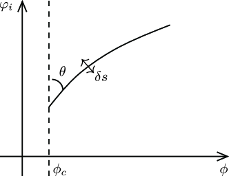
Figure 1: Free light scalar fields ($\varphi_{i}$) are added to the conventional hybrid-type potential. $\delta s$ is the entropy perturbation, and $\theta$ measures the velocity ratio between $\phi$ and the others. Note that $\theta=\pi/2$ is assumed in the original hybrid inflation, but the assumption is not quite obvious when there are many light scalar fields in the model, even if they are decoupled from the hybrid-type potential.

In this paper we consider the perturbation caused by the entropy perturbation $\delta s$. The angled trajectory ($\theta\neq\pi/2$) causes significant creation of the curvature perturbation at the end.

II Free light scalars in hybrid inflation

One might be skeptical about the generation of the curvature perturbation at the end, if it is realized just by adding free scalar fields to the model. To illustrate what happens in this model, we show the simplest calculation, in which one “standard” inflaton $\phi$ and one additional light field $\varphi$ have the same quadratic potential with the same mass $m_{\phi}=m_{\varphi}\equiv m$. Therefore, the potential is given by

$$V(\phi,\sigma)=\frac{\lambda^{2}}{4}\left(\chi^{2}-M^{2}\right)^{2}+\frac{g^{2}}{2}\chi^{2}\phi^{2}+\frac{1}{2}m^{2}(\phi^{2}+\varphi^{2}).$$ (7)

This assumption makes the trajectory straight, and removes ambiguities related to the possible non-trivial evolution of the perturbations during inflation. (See Fig.2.)

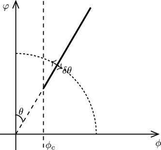
Figure 2: The entropy perturbation leads to $\delta\theta$, which appears along the uniform density hypersurfaces (dotted circle).

Defining the adiabatic field $\sigma^{2}\equiv\phi^{2}+\varphi^{2}$, we find

$$\phi = \sigma\sin\theta$$ (8)

$$\varphi = \sigma\cos\theta.$$ (9)

In this model, the end of inflation defined by the constant $\phi=\phi_{c}$ does not coincide with the uniform density hypersurfaces defined by constant $\sigma$. We find the end is given by

$$\sigma_{e}(\theta)\equiv\frac{\phi_{c}}{\sin\theta},$$ (10)

which is perturbed by $\delta\theta\neq 0$. Therefore, although $\phi_{c}$ is not perturbed in this model, the entropy perturbation ($\delta\theta\neq 0$) causes $\delta N_{e}\neq 0$ at the end of inflation.

The inhomogeneous end of inflation caused by the entropy perturbation is thus given by

$$\delta\sigma_{e} \equiv \frac{\partial\sigma}{\partial\theta}\delta\theta+\frac{1}{2}\frac{\partial^{2}\sigma}{\partial\theta^{2}}(\delta\theta)^{2}+...$$ (11)

$$= -\left[\frac{\cos\theta}{\sin^{2}\theta}\right]\phi_{c}\delta\theta+\frac{1}{2}\left[\frac{1+\cos^{2}\theta}{\sin^{3}\theta}\right]\phi_{c}\left(\delta\theta\right)^{2}+..,$$

$$\simeq -\frac{\cos\theta\phi_{c}}{\sin^{2}\theta}\left(\frac{\delta s}{\sigma}\right)_{*}+\frac{1}{2}\frac{(1+\cos^{2}\theta)\phi_{c}}{\sin^{3}\theta}\left(\frac{\delta s}{\sigma}\right)_{*}^{2}$$

$$= -\frac{1}{\tan\theta}\frac{\sigma_{e}}{\sigma_{*}}\delta s_{*}+\frac{1+\cos^{2}\theta}{2\sin^{2}\theta}\frac{\sigma_{e}}{\sigma_{*}^{2}}\left(\delta s_{*}\right)^{2},$$

where the subscripts “$e$” and “$*$” denote the value at the end of inflation and at the epoch when the perturbation leaves the horizon, respectively. In this simplest example, the relation $\delta\theta=\left[\frac{\delta s}{\sigma}\right]_{*}$ is exact and $\delta\theta$ is constant after the horizon exit. Note that in this formalism $\delta s_{*}$ is Gaussian but $\delta\sigma_{e}$ is not always a Gaussian perturbation.

The curvature perturbation generated at the end of inflation is thus given by

$$\delta N_{e} \equiv H\frac{\delta\sigma_{e}}{\dot{\sigma}_{e}}=-\left[\frac{1}{\eta}\frac{\delta\sigma}{\sigma}\right]_{e}$$ (12)

$$\simeq \frac{1}{\eta_{e}}\frac{1}{\tan\theta}\left(\frac{\delta s}{\sigma}\right)_{*}-\frac{1+\cos^{2}\theta}{2\eta_{e}\sin^{2}\theta}\left(\frac{\delta s}{\sigma}\right)_{*}^{2}.$$

Since the perturbation of the inflation generated at the horizon exit is given by

$$\delta N_{*}=\left[\frac{1}{\eta}\frac{\delta\sigma}{\sigma}\right]_{*},$$ (13)

we find the ratio between the “initial” and “at the end” perturbations;

$$r \equiv \left|\frac{\delta N_{e}}{\delta N_{*}}\right|=\left|\frac{\dot{\sigma}_{*}}{\dot{\sigma}_{e}}\frac{\delta\sigma_{e}}{\delta\sigma_{*}}\right|$$ (14)

$$\simeq \frac{\eta_{*}}{\eta_{e}}\frac{1}{\tan\theta}=\frac{1}{\tan\theta},$$

where the ratio is for the first order perturbations and $\delta s_{*}=\delta\sigma_{*}$ is used for the calculation. We can see that $\delta N_{e}$ dominates (i.e, $r>1$ is realized) when $\tan\theta<1$.

The spectral index $n-1\equiv\partial{\cal P}_{\zeta}/\partial\ln k$ for the perturbation $\delta N_{e}$ is At-the-end

$$n-1\simeq-2\epsilon_{H}+2\eta_{s},$$ (15)

where $\eta_{s}\simeq\eta_{\sigma}\equiv V_{\sigma\sigma}/3H_{*}^{2}$ and $\epsilon_{H}\equiv\dot{H}_{*}/H^{2}_{*}$ are defined at the horizon exit. The spectral index is obviously different from the standard hybrid inflation scenario.

Using the second order perturbation, we can estimate the non-Gaussianity parameter

$$f_{NL}\sim\frac{\eta_{e}}{\cos^{2}\theta},$$ (16)

where $\theta\ll 1$ and $\eta_{e}\ll 1$ suggest $f_{NL}\ll 1$. Here the definition of $f_{NL}$ is

$$f_{NL}\simeq\frac{5}{6}\frac{N_{i}N_{j}N_{ij}}{(N_{m}N_{m})2}+\cdots,$$ (17)

where a subscript $i$ denotes the derivative with respect to the $i$-th field, and “$\cdots$” includes loop corrections that are usually negligible.

Since $f_{NL}$ is obviously small for the quadratic potential, in which $\eta_{*}=\eta_{e}$ is mandatory, we need to consider non-quadratic potential for the enhancement.

One way to enhance $f_{NL}$ is to consider the effective potential that is dominated by the higher polynomial;

$$V(\phi,\varphi)\simeq M^{4}+\alpha_{n}\sigma^{p}.$$ (18)

This potential may allow $\eta_{*}\gg\eta_{e}$, which makes it possible to find $r>1$ and $f_{NL}>1$ at the same time.

II.1 More fields

If there are $N_{f}$ light scalar fields ($\varphi_{i}$, $i=1,...N_{f}$) in the inflationary Universe, a naive statistical expectation is $\theta\sim 1/N_{f}\ll 1$. To avoid the significant creation of $\delta N_{e}$ at the end, these scalar fields must be settled in their minima before the end of inflation, or should have very flat potential compared with the inflaton, so that $\sum_{i=1}^{N_{f}}\dot{\varphi}_{i}^{2}\simeq 0$ is a plausible approximation during inflation.

If there are too many fields in the Universe, N-flation N-flation-paper may start before the onset of hybrid inflation. Then hybrid inflation may begin when $M^{4}$ starts dominating the Universe.

III Free light fields in the spectrum

Above we considered the simplest set-up for the model, in which only one field (adiabatic field) appears in the effective potential during inflation, while the end is caused by the coupling between $\phi$ and $\chi$. However, in more general cases there may be many fields that may have positive/negative mass terms or higher polynomials. Even in that case, the first order perturbation requires very simple parameters. From Fig.3, we can see that for $\delta\theta\ll\theta$ the perturbation at the end of inflation is given by

$$\delta\sigma_{e}\simeq\frac{\delta s_{e}}{\tan\theta},$$ (19)

where we assume $\delta s_{e}\sim\delta s_{*}$. Here $\theta$ is defined by

$$\tan\theta\equiv\frac{|\dot{\phi}|}{\sqrt{\sum_{i=1}^{N_{f}}\dot{\varphi}_{i}^{2}}},$$ (20)

and the adiabatic field $\sigma$ is

$$\dot{\sigma}^{2}\equiv\dot{\phi}^{2}+\sum_{i=1}^{N_{f}}\dot{\varphi}_{i}^{2}.$$ (21)

More general definitions of the adiabatic field (probably including non-canonical kinetic terms matsuda-non-cano ) would be interesting, but they are not the topic in this paper.

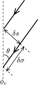
Figure 3: Closer look at the intersection in Fig.1. The perturbed trajectory is approximately parallel when $\delta\theta\ll\theta$.

The curvature perturbation generated at the end of inflation is thus given by

$$\delta N_{e} \simeq H\frac{\delta\sigma_{e}}{\dot{\sigma}_{e}}$$ (22)

$$\simeq \left[\frac{1}{\sqrt{8\pi^{2}\epsilon_{e}}}\frac{H}{M_{p}}\right]\times\frac{1}{\tan\theta_{e}}.$$

Comparing the result with the curvature perturbation generated at the horizon exit ($\delta N_{*}$), we find that $\delta N_{e}$ is enhanced by the factor $1/\tan\theta_{e}\gg 1$.

If one compares this result with the “standard” calculation

$$\delta N_{0}\equiv\left[H\frac{\delta\phi}{\dot{\phi}}\right]_{*}\simeq\left[\frac{1}{\sqrt{8\pi^{2}\epsilon_{\phi}}}\frac{H}{M_{p}}\right],$$ (23)

where the slow-roll parameter $\epsilon_{\phi}$ is defined by $\epsilon_{\phi}\equiv\frac{1}{2}M_{p}^{2}\left(\frac{V_{\phi}}{V}\right)^{2}$, one finds

$$\frac{\delta N_{e}}{\delta N_{0}} \simeq \sqrt{\frac{\epsilon_{\phi}}{\epsilon_{e}}}\frac{1}{\tan\theta_{e}}.$$ (24)

For the simplest (two field, equal mass) model we find

$$\sqrt{\frac{\epsilon_{\phi}}{\epsilon_{e}}}\simeq\sin\theta,$$ (25)

which leads to

$$\frac{\delta N_{e}}{\delta N_{0}} \simeq \cos\theta<1,$$ (26)

or

$$\frac{\delta N_{*}}{\delta N_{0}} \simeq \sin\theta<1.$$ (27)

The minimum ratio $\frac{\delta N_{e}}{\delta N_{0}}\simeq\frac{\delta N_{*}}{\delta N_{0}}\simeq 1/\sqrt{2}$ is obtained when $\tan\theta=1$, where both perturbations contribute (i.e, $\delta N_{*}\simeq\delta N_{e}$). Obviously, the additional light field changes the spectrum.

IV Conclusions and discussions

In the inflationary Universe we may expect many light scalar fields $\varphi_{i}$. Since the adiabatic field during inflation must be defined using all the fields that are moving during inflation, the mismatch between the end of hybrid inflation (usually defined by $\phi$ that is coupled to the waterfall field) and the uniform density hypersurfaces (always defined by the adiabatic field) causes creation of $\delta N$ at the end of inflation. Using the conventional $\delta N$ formalism, we showed that the fields that are decoupled from the inflaton sector can play significant role in creating the curvature perturbation.

The signs of the light fields may appear in the spectral index and/or in the non-Gaussianity, which can be used to discriminate the origin of the perturbation. The precise calculation of these parameters is quite difficult when there are many fields during inflation, but our modest prediction is that the deviation from the standard prediction may indicate the presence of light scalar fields in the early Universe.

In this paper hybrid inflation is simplified assuming that it ends with an instantaneous waterfall starting at the critical instability point $\phi_{c}$. This simplification is not valid if inflation can continue for more than 60 e-folds during the waterfall hyb-alt . However, the model that spends more than 60 e-folds during the waterfall should correspond to hilltop inflation (with probably some modulation caused by the interaction with $\phi$ modulated-inflation ) that should be discriminated from the conventional hybrid inflation scenario.

We discussed the physics related to the evolution before the waterfall using the simplification of the instantaneous waterfall. Our simplification is valid only when the end of inflation mechanism At-the-end is valid for the hybrid inflation model.

V Acknowledgment

We wish to thank K.Shima for encouragement, and our colleagues at Nagoya university and Lancaster university for their kind hospitality.

References

- (1) D. H. Lyth and A. R. Liddle, The primordial density perturbation, Cambridge University Press, 2009.
- (2) F. Bernardeau, L. Kofman and J. -P. Uzan, Phys. Rev. D 70, 083004 (2004) [astro-ph/0403315]; D. H. Lyth, JCAP 0511, 006 (2005) [astro-ph/0510443]; M. P. Salem, Phys. Rev. D 72, 123516 (2005) [astro-ph/0511146].
- (3) M. Sasaki, Prog. Theor. Phys. 120, 159 (2008) [arXiv:0805.0974 [astro-ph]]; A. Naruko and M. Sasaki, Prog. Theor. Phys. 121, 193 (2009) [arXiv:0807.0180 [astro-ph]].
- (4) T. Matsuda, JCAP 0906, 002 (2009) [arXiv:0905.0308 [astro-ph.CO]];
- (5) T. Matsuda, Class. Quant. Grav. 26, 145016 (2009) [arXiv:0906.0643 [hep-th]];
- (6) K. Dimopoulos, K. Kohri, D. H. Lyth and T. Matsuda, arXiv:1110.2951 [astro-ph.CO]; K. Dimopoulos, K. Kohri and T. Matsuda, arXiv:1201.6037 [hep-ph].
- (7) A. R. Liddle, A. Mazumdar, F. E. Schunck, Phys. Rev. D58, 061301 (1998). [astro-ph/9804177]; S. Dimopoulos, S. Kachru, J. McGreevy, J. G. Wacker, JCAP 0808, 003 (2008). [hep-th/0507205].
- (8) T. Matsuda, Phys. Lett. B 682, 163 (2009) [arXiv:0906.2525 [hep-th]]; T. Matsuda, JHEP 0810, 089 (2008) [arXiv:0810.3291 [hep-ph]].
- (9) S. Clesse, Phys. Rev. D 83, 063518 (2011) [arXiv:1006.4522 [gr-qc]].
- (10) T. Matsuda, Phys. Lett. B 665, 338 (2008) [arXiv:0801.2648 [hep-ph]]; T. Matsuda, JCAP 0805, 022 (2008) [arXiv:0804.3268 [hep-th]].