Scalar and Pseudoscalar Glueball Masses within
a Gaussian Wavefunctional Approximation

Abstract

The lowest scalar and pseudoscalar glueball masses are evaluated by means of the time-dependent variational approach to the Yang-Mills gauge theory without fermions in the Hamiltonian formalism within a Gaussian wavefunctional approximation. The glueball mass is calculated as a pole of the propagator for a composite glueball field which consists of two massless gluons. The glueball propagator is here evaluated by using the linear response theory for the composite external glueball field. As a result, a finite glueball mass is obtained through the interaction between two massless gluons, in which the glueball mass depends on the QCD coupling constant $g$ in the nonperturbative form.

1 Introduction

The hadronic and/or quark-gluonic world governed by mainly the strong interaction reveals very fruitful physics such as existence of various possible phases, characteristic dynamical symmetries and various pattern of their symmetry breaking and so on in the hadronic and/or the quark-gluon matter.[1] In the hadronic world which should be basically described by the quantum chromodynamics (QCD), the color confinement is essential and the observed hadrons are mainly ordinary ($3q$)-baryons and ($q{\bar{q}}$)-mesons. However, it is possible that the so-called color-singlet exotic hadrons exist such as ($3q(q{\bar{q}}))$-hadron like pentaquark hadron.[2] It is believed that the color confinement occurs in QCD due to the non-Abelian nature[3] of the gauge interaction. This non-Abelian nature leads to the interaction between gauge fields themselves which represent gluons. Thus, it is interesting to consider a possible color-singlet state which only consists of gluons. This state is called the glueball.

The investigation about glueball has been performed widely in the theoretical side,[4] for example, by using the bag model, the flux tube model, QCD sum rule method, the lattice QCD simulation and so on. Especially, some lattice QCD simulations have given the glueball masses with certain spins and parties. On the other hand, in the experimental side,[5] some candidates of glueball states have been reported. However, the glueball states mix with the normal ($q{\bar{q}}$)-meson states with the same spin and parity. Therefore, the definite information about glueballs such as masses and decay widths is not extracted experimentally until now. Thus, the information about glueballs may be compared with the results obtained by the lattice QCD simulation.

The many theoretical investigations about glueball have been carried out by the use of the effective model of QCD. In their several investigation, the finite gluon mass is assumed in a certain treatment and the background of the model is not so clear because the gluon does not appear explicitly in a certain model. Thus, it may be necessary and interesting to deal with the glueball starting from the QCD Lagrangian itself.

In our previous paper which is refereed to as (I), the time-dependent variational method has been formulated for the Yang-Mills gauge theory without fermions in the Hamiltonian formalism, in which a Gaussian wavefunctional has been adopted as a possible trial state. This method presents an approximate treatment for the Yang-Mills gauge theory within the Gaussian wavefunctional approximation which corresponds to the Hartree approximation. Further, by the help of the linear response theory,[7] it may be possible that an approximation beyond the Hartree approximation, which may correspond to the random phase approximation (RPA) in many-body physics, is obtained in a non-perturbative way. In Ref.TVM00, it was shown that the Goldstone theorem is satisfied in the time-dependent variational approach to the linear sigma model by the help of the linear response theory, while the Goldstone theorem breaks down in the tree-level approximation. Further, in Ref.TsueMatsuda, the pion and sigma meson masses have been calculated by using the linear response theory in the linear sigma model. The same approach is possible to calculate the glueball masses in the QCD without quarks. Since the time-dependent variational method may be suitable for the use of the linear response theory in the quantum field theory, the Hamiltonian formalism is applied. In this paper, starting from the QCD Lagrangian density without quarks, the lowest scalar $(0^{+})$ and pseudoscalar $(0^{-})$ glueball masses are investigated. Then, the glueball masses are obtained reasonably compared with the results of the lattice QCD simulation. The glueball in this paper consists of two massless gluons which interact by the self-interaction due to the characteristic feature of QCD. As a result, through the interaction, the glueball gets mass.

This paper is organized as follows: In the next section, the time-dependent variational approach to the Yang-Mills gauge theory without fermions is summarized following (I). The formalism partially owes to Ref.Vautherin. In §3, the method to calculate the glueball mass is explained. In §4, the lowest scalar and pseudoscalar glueball masses are evaluated in the modified minimal subtraction scheme which is described in detail in Appendix A. Also, the dependence of the glueball masses on the QCD coupling constant is shown. The last section is devoted to a summary and concluding remarks. In Appendix B, it is shown that the decay width may appear if an imaginary part of a response function investigated in this paper is considered seriously. In Appendix C, it is verified that the gluon mass is zero under the approximation used here in this formalism.

2 Recapitulation of the time-dependent variational approach to the Yang-Mills gauge theory without fermions

In this section, the time-dependent variational approach to the $su(N_{c})$ Yang-Mills gauge theory, which has been developed in our paper, is given and summarized following (I) to make this paper be self-contained. In order to formulate the time-dependent variational method, the Hamiltonian formalism is adopted,[11] in which a Gaussian wavefunctional is applied as one of possible trial states. This trial state includes a mean field and quantum fluctuations around it as variational functions. The time-development of the mean field and quantum fluctuations can be described under this Gaussian approximation. The Gaussian state used here corresponds to a squeezed state.

2.1 Hamiltonian formalism of Yang-Mills gauge theory without fermions

As is well known, the $su(N_{c})$ Yang-Mills gauge theory leads to a constrained system. Therefore, it is necessary to impose a constraint conditions. As was discussed in (I), as a result, the Hamiltonian density can be simply expressed[12] so as to be in Eq.(I$\cdot$2$\cdot$10). Namely

$${\cal H}_{0}=\frac{1}{2}\left[\left({\mib E}^{a}\right)^{2}+\left({\mib B}^{a}\right)^{2}\right]\ ,$$ (1)

where roman letters $a$ denotes color indices. Here, we define ${\mib E}^{a}\equiv(E_{x}^{a},E_{y}^{a},E_{z}^{a})$ and so on and

$${\mib E}^{a}=-i\frac{\delta}{\delta{\mib A}^{a}}\ .$$

$${\mib B}^{a}={\mib\nabla}\times{\mib A}^{a}-\frac{1}{2}gf^{abc}{\mib A}^{b}\times{\mib A}^{c}\ ,$$ (2)

where ${\mib A}^{a}$ is a gauge field and its conjugate field is identical with a color-electric field ${\mib E}^{a}$. Also, the color-magnetic field ${\mib B}^{a}$ is introduced and $f^{abc}$ is a structure constant of $su(N_{c})$ Lie algebra. In the functional Schrödinger representation[13] for a field theory,[11] the conjugate momentum field ${\mib E}^{a}$ in the gauge theory is represented as a functional derivative with respect to a gauge field ${\mib A}^{a}$, in which they obey canonical commutation relations: $[\ A_{i}^{a}({\mib x}),\ E_{j}^{b}({\mib y})\ ]=i\delta_{ij}\delta_{ab}\delta^{3}({\mib x}-{\mib y})$.

We formulate the time-dependent variational method for the Yang-Mils gauge theory. Then, it is necessary to introduce a trial state $|{\Phi}\rangle$ for variation. Here, in this paper, the trial wavefunctional is adopted as a Gaussian form as follows:

$$\Phi({\mib A}^{a}) \equiv \langle{{\mib A}^{a}}|\Phi\rangle$$ (3)

$$= {\cal N}^{-1}\exp\left(i\langle{\overline{\mib E}}|{{\mib A}-{\overline{\mib A}}}\rangle\right)\exp\left(-\langle{{\mib A}-{\overline{\mib A}}}|\frac{1}{4G}-i\Sigma|{{\mib A}-{\overline{\mib A}}}\rangle\right)\ ,$$

where ${\cal N}$ is a normalization factor and we use abbreviated notations as

$$\langle{\overline{\mib E}}|{{\mib A}}\rangle=\int d^{3}{\mib x}{\overline{\mib E}}^{a}({\mib x},t)\cdot{\mib A}^{a}({\mib x})\ ,$$

$$\langle{{\mib A}}|\frac{1}{4G}|{{\mib A}}\rangle=\int\!\int\!d^{3}{\mib x}\ d^{3}{\mib y}\ A^{a}_{i}({\mib x})\frac{1}{4}G^{-1}{}^{ab}_{ij}({\mib x},{\mib y},t)A^{b}_{j}({\mib y})\ .$$ (4)

Here, ${\overline{A}}_{i}^{a}({\mib x},t)$, ${\overline{E}}_{i}^{a}({\mib x},t)$, $G_{ij}^{ab}({\mib x},{\mib y},t)$ and $\Sigma_{ij}^{ab}({\mib x},{\mib y},t)$ are the variational functions in which ${\overline{A}}_{i}^{a}({\mib x},t)$ and ${\overline{E}}_{i}^{a}({\mib x},t)$ correspond to the expectation values of the field operators ${A}_{i}^{a}({\mib x})$ and $E_{i}^{a}({\mib x})$, respectively, and two-point functions $G_{ij}^{ab}({\mib x},{\mib y},t)$ and $\Sigma_{ij}^{ab}({\mib x},{\mib y},t)$ are related to the expectation values of the composite operators as follows:

$$\langle{\Phi}|A_{i}^{a}({\mib x})|{\Phi}\rangle={\overline{A}}_{i}^{a}({\mib x},t)\ ,$$

$$\langle{\Phi}|E_{i}^{a}({\mib x})|{\Phi}\rangle={\overline{E}}_{i}^{a}({\mib x},t)\ ,$$

$$\langle{\Phi}|A_{i}^{a}({\mib x})A_{j}^{b}({\mib y})|{\Phi}\rangle={\overline{A}}_{i}^{a}({\mib x},t){\overline{A}}_{j}^{b}({\mib y},t)+G_{ij}^{ab}({\mib x},{\mib y},t)\ ,$$

$$\langle{\Phi}|E_{i}^{a}({\mib x})E_{j}^{b}({\mib y})|{\Phi}\rangle={\overline{E}}_{i}^{a}({\mib x},t){\overline{E}}_{j}^{b}({\mib y},t)+\frac{1}{4}G^{-1}{}_{ij}^{ab}({\mib x},{\mib y},t)+4(\Sigma G\Sigma)_{ij}^{ab}({\mib x},{\mib y},t)\ ,$$

$$\langle{\Phi}|{A}_{i}^{a}({\mib x}){E}_{j}^{b}({\mib y})|{\Phi}\rangle={\overline{A}}_{i}^{a}({\mib x},t){\overline{E}}_{j}^{b}({\mib y},t)+2(G\Sigma)_{ij}^{ab}({\mib x},{\mib y},t)\ .$$ (5)

Thus, it is understood that ${\overline{A}}_{i}^{a}({\mib x},t)$ represents a mean field for the field $A_{i}^{a}({\mib x})$ and a diagonal element of two-point function $G_{ij}^{ab}({\mib x},{\mib y},t)$, namely $G_{ii}^{aa}({\mib x},{\mib x},t)$, represents a quantum fluctuations around the mean field ${\overline{A}}_{i}^{a}({\mib x},t)$. The state $|{\Phi}\rangle$ in (3) is identical with the squeezed state.[14] Thus, in this paper, the lowest excitation mode with a certain quantum number around vacuum is only treated.[9]

To determine the time-dependence of the state $|{\Phi}\rangle$ or a Gaussian wavefunctional $\Phi({\mib A}^{a})$, it is necessary to determine the time-dependence of the variational functions ${\overline{A}}_{i}^{a}({\mib x},t)$, ${\overline{E}}_{i}^{a}({\mib x},t)$, $G_{ij}^{ab}({\mib x},{\mib y},t)$ and $\Sigma_{ij}^{ab}({\mib x},{\mib y},t)$. The time-development of the state under the Hamiltonian density ${\cal H}$ is governed by the time-dependent variational principle in general:

$$\delta\int\!dt\langle{\Phi}|i\frac{\partial}{\partial t}-\int\!d^{3}{\mib x}{\cal H}|{\Phi}\rangle=0\ .$$ (6)

Here, the Hamiltonian derived from the Hamiltonian density (1) can be expressed as

$$\langle H_{0}\rangle \equiv \int d^{3}{\mib x}\langle{\Phi}|{\cal H}_{0}|{\Phi}\rangle$$ (7)

$$= \int d^{3}{\mib x}\biggl{(}\frac{1}{2}{\overline{\mib B}}^{a}({\mib x})\cdot{\overline{\mib B}}^{a}({\mib x})+\frac{1}{2}{\overline{\mib E}}^{a}({\mib x})\cdot{\overline{\mib E}}^{a}({\mib x})+\frac{1}{8}{\rm Tr}\langle{\mib x}|G^{-1}|{\mib x}\rangle$$

$$\qquad\quad+2{\rm Tr}\langle{\mib x}|\Sigma G\Sigma|{\mib x}\rangle+\frac{1}{2}{\rm Tr}\langle{\mib x}|KG|{\mib x}\rangle+\frac{g^{2}}{8}\left({\rm Tr}[S_{i}T^{a}\langle{\mib x}|G|{\mib x}\rangle]\right)^{2}$$

$$\qquad\quad+\frac{g^{2}}{4}{\rm Tr}\left[S_{i}T^{a}\langle{\mib x}|G|{\mib x}\rangle S_{i}T^{a}\langle{\mib x}|G|{\mib x}\rangle\right]\biggl{)}\ ,$$

where

$${\overline{B}}_{i}^{a}=\epsilon_{ijk}\partial_{j}{\overline{A}}_{k}^{a}-\frac{1}{2}gf^{abc}\epsilon_{ijk}{\overline{A}}_{j}^{b}{\overline{A}}_{k}^{c}\ ,$$

$$(S_{i})_{jk}=i\epsilon_{ijk}\ ,\qquad(T^{a})^{bc}=-if^{abc}\ ,$$

$$K=(-i{\mib S}\cdot{\mib D})^{2}-g{\mib S}\cdot{\overline{\mib B}}\ ,$$

$${\mib D}=\nabla-ig{\overline{\mib A}}\ ,\qquad{\overline{A}}_{i}={\overline{A}}_{i}^{a}T^{a}\ ,\quad{\overline{B}}_{i}={\overline{B}}_{i}^{a}T^{a}\ .$$ (8)

Here, $\epsilon_{ijk}$ is a complete antisymmetric tensor and ${\mib S}$ implies a spin 1 matrix. The time-dependent variational principle (6) leads to the following equations of motion:

$${\dot{\overline{\mib A}}}^{a}({\mib x},t)=\frac{\delta\langle H\rangle}{\delta{\overline{\mib E}}^{a}({\mib x},t)}\ ,\qquad{\dot{\overline{\mib E}}}^{a}({\mib x},t)=-\frac{\delta\langle H\rangle}{\delta{\overline{\mib A}}^{a}({\mib x},t)}\ ,$$ (9a)

$${\dot{G}}_{ij}^{ab}({\mib x},{\mib y},t)=\frac{\delta\langle H\rangle}{\delta\Sigma_{ij}^{ab}({\mib x},{\mib y},t)}\ ,\qquad{\dot{\Sigma}}_{ij}^{ab}({\mib x},{\mib y},t)=-\frac{\delta\langle H\rangle}{\delta G_{ij}^{ab}({\mib x},{\mib y},t)}\ ,$$ (9b)

where the dot represents a time-derivative, that is, ${\dot{\overline{\mib A}}}^{a}({\mib x},t)\equiv{\partial{\overline{\mib A}}^{a}({\mib x},t)}/\partial t$ and so on. These equations of motion are identical with the canonical equations of motion since the canonicity conditions,[15] which are developed in the theory of collective motion in nuclei, for the variational functions are implicitly imposed. Under the Hamiltonian density ${\cal H}_{0}$, a possible set of solutions with respect to ${\overline{\mib A}}^{a}$ and ${\overline{\mib E}}^{a}$ is given by

$${\overline{\mib A}}^{a}({\mib x},t)={\overline{\mib E}}^{a}({\mib x},t)={\mib 0}\ .$$ (10)

Instead of the equations of motion for the two-point function $G_{ij}^{ab}({\mib x},{\mib y},t)$ and $\Sigma_{ij}^{ab}({\mib x},{\mib y},t)$ in Eq.(9b), we can reformulate the equations of motion by introducing the reduced density matrix.[16] The reduced density matrix ${\cal M}$ is defined as

$${\cal M}_{ij}^{ab}({\mib x},{\mib y},t) = \left(\begin{array}[]{@{\,}cc@{\,}}-i\langle{\hat{A}}_{i}^{a}({\mib x},t){\hat{E}}_{j}^{b}({\mib y},t)\rangle-\frac{1}{2}&\langle{\hat{A}}_{i}^{a}({\mib x},t){\hat{A}}_{j}^{b}({\mib y},t)\rangle\\ \langle{\hat{E}}_{i}^{a}({\mib x},t){\hat{E}}_{j}^{b}({\mib y},t)\rangle&i\langle{\hat{E}}_{i}^{a}({\mib x},t){\hat{A}}_{j}^{b}({\mib y},t)\rangle-\frac{1}{2}\end{array}\right)$$ (13)

$$= \left(\begin{array}[]{@{\,}cc@{\,}}-2i(G\Sigma)_{ij}^{ab}({\mib x},{\mib y},t)&G_{ij}^{ab}({\mib x},{\mib y},t)\\ \frac{1}{4}(G^{-1})_{ij}^{ab}({\mib x},{\mib y},t)+4(\Sigma G\Sigma)_{ij}^{ab}({\mib x},{\mib y},t)&2i(\Sigma G)_{ij}^{ab}({\mib x},{\mib y},t)\end{array}\right),\qquad\ \$$ (16)

where ${\hat{A}}_{i}^{a}$ and ${\hat{E}}_{i}^{a}$ represent the quantum fluctuations around mean fields, which are defined by

$${\hat{A}}_{i}^{a}({\mib x},t) \equiv A_{i}^{a}({\mib x})-\langle A_{i}^{a}({\mib x})\rangle=A_{i}^{a}({\mib x})-{\overline{A}}_{i}^{a}({\mib x},t)\ ,$$

$${\hat{E}}_{i}^{a}({\mib x},t) \equiv E_{i}^{a}({\mib x})-\langle E_{i}^{a}({\mib x})\rangle=E_{i}^{a}({\mib x})-{\overline{E}}_{i}^{a}({\mib x},t)\ .$$ (17)

As for the reduced density matrix, it has been shown that the time-development of the reduced density matrix is governed by the following Liouville-von Neumann type equation of motion:

$$i{\dot{\cal M}}_{ij}^{ab}({\mib x},{\mib y},t) = [\ {\widetilde{\cal H}}_{0}\ ,\ {\cal M}\ ]_{ij}^{ab}({\mib x},{\mib y},t)\ ,\qquad\qquad\qquad\qquad\qquad\qquad$$ (18a)

where the Hamiltonian matrix $${\widetilde{\cal H}}_{0} {\cal H}_{0}$$ corresponding to is introduced as

$${\widetilde{\cal H}}_{0}{}_{ij}^{ab}({\mib x},{\mib y},t) = \left(\begin{array}[]{@{\,}cc@{\,}}0&\delta_{ij}\delta_{ab}\\ \Gamma_{ij}^{ab}({\mib x},t)&0\end{array}\right)\delta^{3}({\mib x}-{\mib y})\ ,$$ (18d)

$$\Gamma_{ij}^{ab}({\mib x},t) = K_{ij}^{ab}+g^{2}\left(S_{k}T^{c}\langle{{\mib x}}|G|{\mib x}\rangle S_{k}T^{c}\right)_{ij}^{ab}+\frac{g^{2}}{2}\left(S_{k}T^{c}\right)_{ij}^{ab}{\rm Tr}\left[S_{k}T^{c}\langle{\mib x}|G|{\mib x}\rangle\right]\ .$$

The reduced density matrix (13) satisfies the following relation:

$${\cal M}^{2}=\left(\begin{array}[]{@{\,}cc@{\,}}\frac{1}{4}&0\\ 0&\frac{1}{4}\end{array}\right)\ .$$ (21)

Therefore, it is concluded that the eigenvalue of the reduced density matrix ${\cal M}$ itself is $+1/2$ or $-1/2$. Let the eigenstate for ${\cal M}$ be $|{\sigma 1/2,n,a,i}\rangle$ where $\sigma=\pm$ and $n$ represents a certain quantum number. Thus, the eigenvalue equation for ${\cal M}$ is written as

$${\cal M}_{ij}^{ab}|{\sigma 1/2,n,b,j}\rangle=\sigma\frac{1}{2}|{\sigma 1/2,n,a,i}\rangle\ .$$ (22)

Then, let us introduce the mode functions $u$ and $v$ in the coordinate representation by using the eigenstates for ${\cal M}$:

$$\langle{\mib x}|+1/2,n,a,i\rangle=\left(\begin{array}[]{@{\,}c@{\,}}u_{n}{}_{i}^{a}({\mib x},t)\\ v_{n}{}_{i}^{a}({\mib x},t)\end{array}\right)\ .$$ (23)

Then, it is possible to express the reduced density matrix in terms of the above mode functions, namely, the spectral decomposition can be carried out:

$${\cal M}_{ij}^{ab}({\mib x},{\mib y},t) = \sum_{n(\sigma>0)}f_{n}\biggl{[}\left(\begin{array}[]{@{\,}c@{\,}}u_{n}{}_{i}^{a}({\mib y},t)\\ v_{n}{}_{i}^{a}({\mib y},t)\end{array}\right)(\ v_{n}^{*}{}_{j}^{b}({\mib y})\ ,\ u_{n}^{*}{}_{j}^{b}({\mib y})\ )$$ (29)

$$\qquad\qquad+\left(\begin{array}[]{@{\,}c@{\,}}u^{*}_{n}{}_{i}^{a}({\mib y},t)\\ -v^{*}_{n}{}_{i}^{a}({\mib y},t)\end{array}\right)(\ -v_{n}{}_{j}^{b}({\mib y})\ ,\ u_{n}{}_{j}^{b}({\mib y})\ )\biggl{]}\ ,$$

where $f_{n}=1/2$. Here, the mode functions satisfy the following orthonormalized conditions as

$$\sum_{a,i}\int d^{3}{\mib x}\left(v^{*}_{n^{\prime}}{}_{i}^{a}({\mib x})u_{n}{}_{i}^{a}({\mib x})+u^{*}_{n^{\prime}}{}_{i}^{a}({\mib x})v_{n}{}_{i}^{a}({\mib x})\right)=\delta_{nn^{\prime}}\ ,$$

$$\sum_{a,i}\int d^{3}{\mib x}\left(u^{*}_{n^{\prime}}{}_{i}^{a}({\mib x})v^{*}_{n}{}_{i}^{a}({\mib x})-v^{*}_{n^{\prime}}{}_{i}^{a}({\mib x})u^{*}_{n}{}_{i}^{a}({\mib x})\right)=0\ ,$$

$$\sum_{a,i}\int d^{3}{\mib x}\left(u_{n^{\prime}}{}_{i}^{a}({\mib x})v_{n}{}_{i}^{a}({\mib x})-v_{n^{\prime}}{}_{i}^{a}({\mib x})u_{n}{}_{i}^{a}({\mib x})\right)=0\ .$$ (30)

For the equation of motion (18a), if the reduced density matrix ${\cal M}={\cal M}_{0}$ has no time-dependence, the equation of motion is reduced to $[\ {\widetilde{\cal H}}_{0}\ ,\ {\cal M}_{0}\ ]=0$, namely, the reduced density matrix and the Hamiltonian matrix is commutable each other. In this situation, it is possible to diagonalize ${\cal M}_{0}$ and ${\widetilde{\cal H}}_{0}$ simultaneously. Thus, the diagonal basis $|{ai{\mib k}\sigma}\rangle$ can be introduced, where the following relations are satisfied:

$${\hat{\cal H}}_{0}|{ai{\mib k}\sigma}\rangle=E_{\bf k}^{\sigma}|{ai{\mib k}\sigma}\rangle\ ,\qquad{\hat{\cal M}}_{0}|{ai{\mib k}\sigma}\rangle=f_{\bf k}^{\sigma}|{ai{\mib k}\sigma}\rangle\ ,$$

$$\qquad E_{\bf k}^{\sigma}=\sigma E_{\bf k}\ ,\qquad f_{\bf k}^{\sigma}=\sigma\cdot\frac{1}{2}\ ,\qquad\sigma=\pm\ .$$

Here, the second equation in Eq.(2.1) is identical with Eq.(22), so the diagonal basis is nothing but $|{\sigma 1/2,n={\mib k},a,i}\rangle$:

$$|{ai{\mib k}\sigma}\rangle=|{\sigma 1/2,{\mib k},a,i}\rangle\ .$$ (32)

The Hamiltonian matrix and the reduced density matrix are diagonalized by using the mode functions in the momentum representation such as

$$U^{-1}{\cal H}_{0}U=\left(\begin{array}[]{@{\,}cc@{\,}}E_{\bf k}&0\\ 0&-E_{\bf k}\end{array}\right)\ ,\qquad U^{-1}{\cal M}_{0}U=\left(\begin{array}[]{@{\,}cc@{\,}}\frac{1}{2}&0\\ 0&-\frac{1}{2}\end{array}\right)\ .$$ (37)

Here, a unitary matrix $U$ in the momentum space is obtained as

$$U({\mib k})_{ij}^{ab}=\left(\begin{array}[]{@{\,}cc@{\,}}u({\mib k})_{ij}^{ab}&u^{*}({\mib k}){}_{ij}^{ab}\\ v({\mib k})_{ij}^{ab}&-v^{*}({\mib k}){}_{ij}^{ab}\end{array}\right)\ ,\qquad U^{-1}({\mib k})_{ij}^{ab}=\left(\begin{array}[]{@{\,}cc@{\,}}v^{*}({\mib k}){}_{ij}^{ab}&u^{*}({\mib k}){}_{ij}^{ab}\\ v({\mib k})_{ij}^{ab}&-u({\mib k}){}_{ij}^{ab}\end{array}\right)\ ,\qquad$$ (42)

where

$$u({\mib k})_{ij}^{ab}=u_{{\bf k}}{}_{i}^{a}\delta_{ij}\delta_{ab}\ ,\qquad v({\mib k})_{ij}^{ab}=v_{{\bf k}}{}_{i}^{a}\delta_{ij}\delta_{ab}\ ,$$ (43)

$$\left(\begin{array}[]{@{\,}c@{\,}}u_{\bf k}{}_{i}^{a}\ ,v_{\bf k}{}_{i}^{a}\end{array}\right)=\langle{\mib k}|1/2,{\mib k},a,i\rangle=\left(\frac{1}{\sqrt{2E_{\bf k}}}\ ,\sqrt{\frac{E_{\bf k}}{2}}\ \right)\ ,$$ (45)

$$E_{\bf k}=|{\mib k}|\ .$$

In the diagonal basis, the Hamiltonian matrix and the reduced density matrix are expressed in the forms of the diagonal matrices as (37). Originally, both are expressed in the form of Eqs.(18d) and (13), respectively. The relation between the original basis $\{|\!|{\alpha}\rangle\}$, which we implicitly used in Eqs.(18d) and (13), and the diagonal basis $\{|{ai{\mib k}\sigma}\rangle\}$ is given by the relation

$$|\!|{\alpha}\rangle\equiv U^{-1}|{ai{\mib k}\sigma}\rangle\ .$$ (46)

3 Scalar and pseudoscalar glueball masses

In this section, a scalar and pseudoscalar glueball masses are calculated in the framework of the time-dependent variational method within the Gaussian approximation developed in the previous section. In general, the propagator $S$ can be obtained by using the generating function of the connected Green function, $W[J]$, as

$$S=\frac{\delta^{2}W[J]}{\delta J\delta J}\ ,$$ (47)

where $J$ represents a source current. Here, since the expectation value of the field operator $\varphi$ is obtained as $\varphi=\delta W[J]/\delta J$, the propagator can be expressed as

$$S_{IJ}=\frac{\delta\varphi_{I}}{\delta J_{J}}\ ,$$ (48)

where the subscripts $I$ and $J$ imply certain indices. In our Hamiltonian formalism, we introduce the external field $\varphi_{I}({\mib x})$ with a source current $J_{I}(x)$, and the external Hamiltonian $H_{\rm ext}$ should be added to the Hamiltonian $H_{0}$:

$$H_{\rm ext}=\int d^{3}{\mib x}J_{I}({\mib x},t)\varphi_{I}({\mib x})=\epsilon e^{-i\omega t}\int d^{3}{\mib x}e^{i{\bf q}\cdot{\bf x}}{J}_{I}{\varphi}_{I}({\mib x})\ ,$$ (49)

where the source current $J_{I}(x)$ is assumed as $J_{I}(x)=\epsilon e^{-iqx}J_{I}$. Thus, as for the expectation value of the field operator $\varphi_{I}$ which we write $\langle\varphi_{I}\rangle$, the same time- and coordinate-dependence as that of the source current is expected:

$$\langle{\varphi}_{I}({\mib x})\rangle=\beta_{I}e^{-i\omega t+i{\bf q}\cdot{\bf x}}\ .$$ (50)

Therefore, the propagator $S_{IJ}$ is evaluated by

$$S_{IJ}=\lim_{\epsilon\rightarrow 0}\frac{\beta_{I}}{\epsilon J_{J}}\ .$$ (51)

Namely, a mass of particle represented by the field operator $\varphi_{I}$ is calculated as a pole of the propagator, namely, the pole of $\lim_{\epsilon\rightarrow 0}\beta_{I}/\epsilon$.[8]

Under the existence of the source current $J_{I}$, the reduced density matrix ${\cal M}$ is shifted from ${\cal M}_{0}$ which means the reduced density matrix without the source term. Of course, the Hamiltonian matrix ${\widetilde{\cal H}}$ is also shifted:

$${\widetilde{\cal H}}={\widetilde{\cal H}}_{0}+\delta{\widetilde{\cal H}}\ ,$$

$${\cal M}={\cal M}_{0}+\delta{\cal M}\ ,$$ (52)

where the quantities with subscript 0 represent those without the source term. Since the change of the reduced density matrix leads to the change of its (1,2)-component, $G_{ij}^{ab}$ in Eq.(13), then the Hamiltonian matrix which contains $G_{ij}^{ab}$ is also changed through $\Gamma_{ij}^{ab}$ in Eqs.(18d) and (LABEL:2-13c), namely $\Gamma_{ij}^{ab}\rightarrow\Gamma_{ij}^{ab}+\delta\Gamma_{ij}^{ab}$. Thus, up to the order of $\epsilon$, the Liouville von-Neumann type equation of motion for the reduced density matrix can be expressed as

$$i\delta{\dot{\cal M}}=[\ {\widetilde{\cal H}}_{0}\ ,\ \delta{\cal M}\ ]+[\ \delta{\widetilde{\cal H}}_{\rm ext}\ ,\ {\cal M}_{0}\ ]+[\ \delta{\widetilde{\cal H}}_{\rm ind}\ ,\ {\cal M}_{0}\ ]\ ,$$ (53)

$$\delta{\widetilde{\cal H}}_{\rm ind}=\left(\begin{array}[]{@{\,}cc@{\,}}0&\delta_{ij}\delta_{ab}\\ \delta\Gamma_{ij}^{ab}&0\end{array}\right)\ .$$ (56)

Here, the shift of the Hamiltonian matrix, $\delta{\widetilde{\cal H}}$, is divided into two parts, namely $\delta{\widetilde{\cal H}}=\delta{\widetilde{\cal H}}_{\rm ind}+\delta{\widetilde{\cal H}}_{\rm ext}$, in which $\delta{\widetilde{\cal H}}_{\rm ind}$ represents the shift due to $\delta\Gamma$ and $\delta{\widetilde{\cal H}}_{\rm ext}$ represents the shift occurring directly from the introduction of the external Hamiltonian $H_{\rm ext}$.

3.1 Scalar glueball mass: $0^{+}$

The scalar glueball field is constructed as the following composite operator:

$$\varphi_{I}\equiv\frac{1}{2}F_{\mu\nu}^{a}F_{a}^{\mu\nu}={E}_{i}^{a}{E}_{i}^{a}+B_{i}^{a}B_{i}^{a}\ .$$ (57)

As for the external field $B_{i}^{a}B_{i}^{a}$, the response $\delta{\cal M}$ has the same form as that for $E_{i}^{a}E_{i}^{a}$ in our Gaussian approximation. Thus, we adopt the external Hamiltonian simply as follows:

$$H_{\rm ext}=\int d^{3}{\mib x}\int d^{3}{\mib y}{J}_{ij}^{ab}({\mib x},{\mib y},t)E_{i}^{a}({\mib x})E_{j}^{b}({\mib y})\ ,$$ (58)

where the source current $J_{ij}^{ab}({\mib x},{\mib y},t)$ is proportional to $\delta_{ij}\delta_{ab}\delta^{3}({\mib x}-{\mib y})$ for $0^{+}$ glueball state. We can derive the Liouville-von Neumann type equation of motion for the reduced density matrix as is similar to Eq.(18a).

$$i{\dot{\cal M}}_{ij}^{ab}({\mib x},{\mib y},t) = [\ {\widetilde{\cal H}}_{J}\ ,\ {\cal M}\ ]_{ij}^{ab}({\mib x},{\mib y},t)\ ,$$ (59)

$${\widetilde{\cal H}}_{J} = {\widetilde{\cal H}}_{0}+\delta{\widetilde{\cal H}}_{\rm ext}+\delta{\widetilde{\cal H}}_{\rm ind}\ ,$$

where

$$\delta{\widetilde{\cal H}}_{\rm ext}{}_{ij}^{ab}({\mib x},{\mib y},t)=\left(\begin{array}[]{@{\,}cc@{\,}}0&2J_{ij}^{ab}({\mib x},{\mib y},t)\\ 0&0\end{array}\right)\ .$$ (62)

By using the equation $[\ {\widetilde{\cal H}}_{0}\ ,\ {\cal M}_{0}\ ]=0$ and, first, omitting the induced term $\delta{\widetilde{\cal H}}_{\rm ind}$, the following equation of motion is obtained:

$$i\delta{\dot{\cal M}}=[\ {\widetilde{\cal H}}_{0}\ \ ,\ \delta{\cal M}\ ]+[\ \delta{\widetilde{\cal H}}_{\rm ext}\ ,\ {\cal M}_{0}\ ]\ .$$ (63)

We call $\delta{\cal M}$ derived by neglecting the induced term the bare response.

Let us take the source current in the form

$$J_{ij}^{ab}({\mib x},{\mib y},t)={\widetilde{J}}_{ij}^{ab}e^{-i\omega t+i{\bf q}\cdot{\bf x}}\delta^{3}({\mib x}-{\mib y})\ .$$ (64)

Since $\delta{\widetilde{\cal H}}_{\rm ext}$ is proportional to $e^{-i\omega t+i{\mib q}\cdot{\mib x}}$, then, the bare response $\delta{\cal M}$ is also proportional to $e^{-i\omega t+i{\mib q}\cdot{\mib x}}$, which leads to $i\delta{\dot{\cal M}}=\omega\delta{\cal M}$. Thus, by using the diagonal basis $\{|{ai{\mib k}\sigma}\rangle\}$ which obeys the eigenvalue equations in (2.1), Eq.(63) is recast into

$$\langle{ai{\mib k}\sigma}|\delta{\cal M}|{bj{\mib k}^{\prime}\sigma^{\prime}}\rangle=\frac{f_{{\bf k}^{\prime}}^{{\sigma}^{\prime}}-f_{{\bf k}}^{\sigma}}{\omega-(E_{\bf k}^{\sigma}-E_{{\bf k}^{\prime}}^{{\sigma}^{\prime}})}\langle{ai{\mib k}\sigma}|\delta{\widetilde{\cal H}}_{\rm ext}|{bj{\mib k}^{\prime}\sigma^{\prime}}\rangle\ .$$ (65)

Here, we can rewrite the matrix elements in terms of the original basis as

$$\langle{ai{\mib k}\sigma}|\delta{\widetilde{\cal H}}_{\rm ext}|{bj{\mib k}^{\prime}\sigma^{\prime}}\rangle = \sum_{\alpha,\beta}\langle{ai{\mib k}\sigma}|\alpha\rangle\!\rangle\langle\!\langle{\alpha}|\delta{\widetilde{\cal H}}_{\rm ext}|{\beta}\rangle\!\rangle\langle\!\langle\beta|{bj{\mib k}^{\prime}\sigma^{\prime}}\rangle$$ (68)

$$= U^{-1}({\mib k})_{il}^{ae}\left(\begin{array}[]{@{\,}cc@{\,}}0&2J_{lm}^{ef}\\ 0&0\end{array}\right)U({\mib k}^{\prime})_{mj}^{fb}$$

$$= \left(\begin{array}[]{@{\,}cc@{\,}}2v({\bf k})^{*}{}_{il}^{ae}{\widetilde{J}}_{lm}^{ef}v({{\bf k}^{\prime}}){}_{mj}^{fb}&-2v({\bf k})^{*}{}_{il}^{ae}{\widetilde{J}}_{lm}^{ef}v({{\bf k}^{\prime}})^{*}{}_{mj}^{fb}\\ 2v({\bf k}){}_{il}^{ae}{\widetilde{J}}_{lm}^{ef}v({{\bf k}^{\prime}}){}_{mj}^{fb}&-2v({\bf k}){}_{il}^{ae}{\widetilde{J}}_{lm}^{ef}v({{\bf k}^{\prime}})^{*}{}_{mj}^{fb}\end{array}\right)_{\!\!\sigma\sigma^{\prime}}\!\!\!\!\langle{\mib k}|e^{-iqx}|{{\mib k}^{\prime}}\rangle$$ (71)

$$= \left[\left(\begin{array}[]{@{\,}c@{\,}}v_{\bf k}^{*}{}_{i}^{a}\\ v_{\bf k}{}_{i}^{a}\end{array}\right)2{\widetilde{J}}_{ij}^{ab}(q)\left(\begin{array}[]{@{\,}cc@{\,}}v_{{\bf k}^{\prime}}{}_{j}^{b}&-v_{{\bf k}^{\prime}}^{*}{}_{j}^{b}\end{array}\right)\right]_{\sigma\sigma^{\prime}}\!\!\delta^{3}({\mib k}^{\prime}-{\mib k}+{\mib q})e^{-i\omega t}.$$ (75)

As is similar to the above transformation, inversely, the shift of the reduced density matrix $\delta{\cal M}$ can be expressed in terms of the diagonal basis as

$$\delta{\cal M} = \left(\begin{array}[]{@{\,}cc@{\,}}-i\delta\langle{\hat{A}}_{i}^{a}{\hat{E}}_{j}^{b}\rangle&\delta\langle{\hat{A}}_{i}^{a}{\hat{A}}_{j}^{b}\rangle\\ \delta\langle{\hat{E}}_{i}^{a}{\hat{E}}_{j}^{b}\rangle&i\delta\langle{\hat{E}}_{i}^{a}{\hat{A}}_{j}^{b}\rangle\end{array}\right)$$ (78)

$$= U({\mib k})_{il}^{ae}\left(\begin{array}[]{@{\,}cc@{\,}}\langle{el{\mib k}+}|\delta{\cal M}|{mf{\mib k}^{\prime}+}\rangle&\langle{el{\mib k}+}|\delta{\cal M}|{mf{\mib k}^{\prime}-}\rangle\\ \langle{el{\mib k}-}|\delta{\cal M}|{mf{\mib k}^{\prime}+}\rangle&\langle{el{\mib k}-}|\delta{\cal M}|{mf{\mib k}^{\prime}-}\rangle\end{array}\right)U^{-1}({\mib k}^{\prime})_{mj}^{fb}\ .\quad$$ (81)

Thus, we obtain the shift of $G_{ij}^{ab}$ and so on such as

$$\delta\langle{\hat{A}}_{i}^{a}{\hat{A}}_{j}^{b}\rangle = u_{\bf k}{}_{i}^{a}\langle{ai{\mib k}+}|\delta{\cal M}|{bj{\mib k}^{\prime}+}\rangle u_{{\bf k}^{\prime}}^{*}{}_{j}^{b}+u_{\bf k}^{*}{}_{i}^{a}\langle{ai{\mib k}-}|\delta{\cal M}|{bj{\mib k}^{\prime}+}\rangle u_{{\bf k}^{\prime}}^{*}{}_{j}^{b}$$

$$-u_{\bf k}{}_{i}^{a}\langle{ai{\mib k}+}|\delta{\cal M}|{bj{\mib k}^{\prime}-}\rangle u_{{\bf k}^{\prime}}{}_{j}^{b}-u_{\bf k}^{*}{}_{i}^{a}\langle{ai{\mib k}-}|\delta{\cal M}|{bj{\mib k}^{\prime}-}\rangle u_{{\bf k}^{\prime}}{}_{j}^{b}\ ,$$

$$\equiv \delta{\cal G}_{+-}{}_{ij}^{ab}({\mib k},{\mib k}-{\mib q})\delta^{3}({\mib k}^{\prime}-{\mib k}+{\mib q})e^{-i\omega t}$$

$$\delta\langle{\hat{E}}_{i}^{a}{\hat{E}}_{j}^{b}\rangle = v_{\bf k}{}_{i}^{a}\langle{ai{\mib k}+}|\delta{\cal M}|{bj{\mib k}^{\prime}+}\rangle v_{{\bf k}^{\prime}}^{*}{}_{j}^{b}-v_{\bf k}^{*}{}_{i}^{a}\langle{ai{\mib k}-}|\delta{\cal M}|{bj{\mib k}^{\prime}+}\rangle v_{{\bf k}^{\prime}}^{*}{}_{j}^{b}$$ (82)

$$+v_{\bf k}{}_{i}^{a}\langle{ai{\mib k}+}|\delta{\cal M}|{bj{\mib k}^{\prime}-}\rangle v_{{\bf k}^{\prime}}{}_{j}^{b}-v_{\bf k}^{*}{}_{i}^{a}\langle{ai{\mib k}-}|\delta{\cal M}|{bj{\mib k}^{\prime}-}\rangle v_{{\bf k}^{\prime}}{}_{j}^{b}$$

$$\equiv \delta{\cal G}_{-+}{}_{ij}^{ab}({\mib k},{\mib k}-{\mib q})\delta^{3}({\mib k}^{\prime}-{\mib k}+{\mib q})e^{-i\omega t}$$

with (65) and (68).

Next, let us include the induced term $\delta{\widetilde{\cal H}}_{\rm ind}$. First, the shift of $G_{ij}^{ab}({\mib x},{\mib x})$ is calculated from Eq.(3.1) as

$$\delta G_{ij}^{ab}({\mib x},{\mib x}) = \langle{\mib x}|\delta({\hat{A}}_{i}^{a}{\hat{A}}_{j}^{b})|{\mib x}\rangle=\int d^{3}{\mib k}\int d^{3}{\mib k}^{\prime}\langle{\mib x}|{\mib k}\rangle\langle{\mib k}|\delta({\hat{A}}_{i}^{a}{\hat{A}}_{j}^{b})|{{\mib k}^{\prime}}\rangle\langle{{\mib k}^{\prime}}|{\mib x}\rangle$$ (83)

$$= \int d^{3}{\mib k}\int d^{3}{\mib k}^{\prime}\frac{e^{{i({\bf k}-{\bf k}^{\prime}})\cdot{\bf x}}}{(2\pi)^{3}}\langle{\mib k}|\delta({\hat{A}}_{i}^{a}{\hat{A}}_{j}^{b})|{{\mib k}^{\prime}}\rangle$$

$$= e^{i{\bf q}\cdot{\bf x}}\int\frac{d^{3}{\mib k}}{(2\pi)^{3}}\delta{\cal G}_{+-}{}_{ij}^{ab}({\mib k},{\mib k}-{\mib q})e^{-i\omega t}$$

$$\equiv \alpha_{ij}^{ab}(q)e^{-iqx}\ .$$

Similarly,

$$\delta S_{ij}^{ab}({\mib x},{\mib x}) \equiv \langle{\mib x}|\delta({\hat{E}}_{i}^{a}{\hat{E}}_{j}^{b})|{\mib x}\rangle=\int d^{3}{\mib k}\int d^{3}{\mib k}^{\prime}\langle{\mib x}|{\mib k}\rangle\langle{\mib k}|\delta({\hat{E}}_{i}^{a}{\hat{E}}_{j}^{b})|{{\mib k}^{\prime}}\rangle\langle{{\mib k}^{\prime}}|{\mib x}\rangle$$ (84)

$$= \int d^{3}{\mib k}\int d^{3}{\mib k}^{\prime}\frac{e^{{i({\bf k}-{\bf k}^{\prime}})\cdot{\bf x}}}{(2\pi)^{3}}\langle{\mib k}|\delta({\hat{E}}_{i}^{a}{\hat{E}}_{j}^{b})|{{\mib k}^{\prime}}\rangle$$

$$= e^{i{\bf q}\cdot{\bf x}}\int\frac{d^{3}{\mib k}}{(2\pi)^{3}}\delta{\cal G}_{-+}{}_{ij}^{ab}({\mib k},{\mib k}-{\mib q})e^{-i\omega t}$$

$$\equiv \beta_{ij}^{ab}(q)e^{-iqx}\ .$$

Thus, the shift of $\Gamma_{ij}^{ab}$ in the Hamiltonian matrix, $\delta\Gamma_{ij}^{ab}$ in Eq.(53), is given in the momentum representation as

$$\langle{\mib k}|\delta\Gamma_{ij}^{ab}|{{\mib k}^{\prime}}\rangle = \delta\Gamma_{ij}^{ab}(\omega,{\mib q})\delta^{3}({\mib k}^{\prime}-{\mib k}+{\mib q})e^{-i\omega t}$$

$$\delta\Gamma_{ij}^{ab}(\omega,{\mib q}) = \int\frac{d^{3}{\mib k}}{(2\pi)^{3}}\biggl{[}g^{2}\left(S_{k}T^{c}\cdot\delta{\cal G}_{+-}({\mib k},{\mib k}-{\mib q})\cdot S_{k}T^{c}\right)_{ij}^{ab}$$ (85)

$$\qquad\qquad\qquad+\frac{g^{2}}{2}(S_{k}T^{c})_{ij}^{ab}{\rm Tr}\ \left[S_{k}T^{c}\cdot\delta{\cal G}_{+-}({\mib k},{\mib k}-{\mib q})\right]\biggl{]}\ .$$

Here, from Eq.(83), we obtain $\alpha_{ij}^{ab}(q)\equiv\int\frac{d^{3}{\bf k}}{(2\pi)^{3}}\delta{\cal G}_{+-}{}_{ij}^{ab}({\bf k},{\bf k}-{\bf q})$. Thus, $\delta\Gamma_{ij}^{ab}(q)$ can be expressed as follows:

$$\delta\Gamma_{ij}^{ab}(\omega,{\mib q}) = g^{2}(S_{k})_{il}(T^{c})^{ae}\alpha_{lm}^{ef}(q)(S_{k})_{mj}(T^{c})^{fb}$$ (86)

$$+\frac{g^{2}}{2}(S_{k})_{ij}(T^{c})^{ab}\left[(S_{k})_{lm}(T^{c})^{ef}\alpha_{ml}^{fe}(q)\right]\ .$$

Further, the induced term of the Hamiltonian matrix is obtained in the diagonal basis as

$$\langle{ai{\mib k}\sigma}|\delta{\widetilde{\cal H}}_{\rm ind}|{bj{\mib k}^{\prime}\sigma^{\prime}}\rangle = U^{-1}({\mib k})_{il}^{ae}\left(\begin{array}[]{@{\,}cc@{\,}}0&0\\ \delta\Gamma_{lm}^{ef}&0\end{array}\right)U({\mib k}^{\prime})_{mj}^{fb}$$ (89)

$$= \left(\begin{array}[]{@{\,}cc@{\,}}u({\bf k})^{*}{}_{il}^{ae}{\delta\Gamma}(q)_{lm}^{ef}u({{\bf k}^{\prime}}){}_{mj}^{fb}&u({\bf k})^{*}{}_{il}^{ae}{\delta\Gamma}(q)_{lm}^{ef}u({{\bf k}^{\prime}})^{*}{}_{mj}^{fb}\\ -u({\bf k}){}_{il}^{ae}{\delta\Gamma}(q)_{lm}^{ef}u({\bf k}^{\prime}){}_{mj}^{fb}&-u({\bf k}){}_{il}^{ae}{\delta\Gamma}(q)_{lm}^{ef}u({{\bf k}^{\prime}})^{*}{}_{mj}^{fb}\end{array}\right)_{\sigma\sigma^{\prime}}$$

$$\qquad\qquad\qquad\qquad\qquad\qquad\qquad\qquad\times\delta^{3}({\mib k}^{\prime}-{\mib k}+{\mib q})e^{-i\omega t}$$

$$= \left[\left(\begin{array}[]{@{\,}c@{\,}}u_{\bf k}^{*}{}_{i}^{a}\\ -u_{\bf k}{}_{i}^{a}\end{array}\right)\delta\Gamma_{ij}^{ab}(q)\left(\begin{array}[]{@{\,}cc@{\,}}u_{{\bf k}^{\prime}}{}_{j}^{b}&u_{{\bf k}^{\prime}}^{*}{}_{j}^{b}\end{array}\right)\right]_{\sigma\sigma^{\prime}}\!\!\delta^{3}({\mib k}^{\prime}-{\mib k}+{\mib q})e^{-i\omega t}\ .$$ (96)

Thus, from the equation of motion (53), we can obtain the response $\delta{\cal M}$ in the diagonal basis in the same way that the bare response was derived in Eq.(78):

$$\langle{ai{\mib k}\sigma}|\delta{\cal M}|{bj{\mib k}^{\prime}\sigma^{\prime}}\rangle$$ (105)

$$= \frac{f_{{\bf k}^{\prime}}^{{\sigma}^{\prime}}-f_{\bf k}^{\sigma}}{\omega-(E_{\bf k}^{\sigma}-E_{{\bf k}^{\prime}}^{\sigma^{\prime}})}\left[\langle{ai{\mib k}\sigma}|\delta{\widetilde{\cal H}}_{\rm ind}|{bj{\mib k}^{\prime}\sigma^{\prime}}\rangle+\langle{ai{\mib k}\sigma}|\delta{\widetilde{\cal H}}_{\rm ext}|{bj{\mib k}^{\prime}\sigma^{\prime}}\rangle\right]$$

$$= \frac{f_{{\bf k}^{\prime}}^{{\sigma}^{\prime}}-f_{\bf k}^{\sigma}}{\omega-(E_{\bf k}^{\sigma}-E_{{\bf k}^{\prime}}^{\sigma^{\prime}})}$$

$$\times\left[\left(\begin{array}[]{@{\,}c@{\,}}u_{\bf k}^{*}{}_{i}^{a}\\ -u_{\bf k}{}_{i}^{a}\end{array}\right)\delta\Gamma_{ij}^{ab}(q)\left(\begin{array}[]{@{\,}cc@{\,}}u_{{\bf k}^{\prime}}{}_{j}^{b}&u_{{\bf k}^{\prime}}^{*}{}_{j}^{b}\end{array}\right)+\left(\begin{array}[]{@{\,}c@{\,}}v_{\bf k}^{*}{}_{i}^{a}\\ v_{\bf k}{}_{i}^{a}\end{array}\right)2{\widetilde{J}}_{ij}^{ab}(q)\left(\begin{array}[]{@{\,}cc@{\,}}v_{{\bf k}^{\prime}}{}_{j}^{b}&-v_{{\bf k}^{\prime}}^{*}{}_{j}^{b}\end{array}\right)\right]_{\sigma\sigma^{\prime}}$$

$$\qquad\qquad\qquad\qquad\qquad\qquad\qquad\qquad\qquad\times\delta^{3}({\mib k}^{\prime}-{\mib k}+{\mib q})e^{-i\omega t}\ .$$

Now, let us return to evaluating the scalar glueball mass. Since the field operator representing the scalar glueball is in Eq.(57), the source current (64) should be applied as follows:

$${\widetilde{J}}_{ij}^{ab}=\epsilon\delta_{ij}\delta_{ab}\ .$$ (106)

In this case, the structure of the Lorentz and color indices of the response is the same one as ${\widetilde{J}}_{ij}^{ab}$ such as $\alpha_{ij}^{ab}\propto\delta_{ij}\delta_{ab}$. Namely,

$$\delta G_{ij}^{ab}(\omega,{\mib q})=\alpha_{ij}^{ab}(q)=\alpha_{i}(q)\delta_{ij}\delta^{ab}\ ,\qquad\beta_{ij}^{ab}(q)=\beta_{i}(q)\delta_{ij}\delta^{ab}\ .$$ (107)

Then, the shift $\delta\Gamma_{ij}^{ab}$ in Eq.(86) is simply written as

$$\delta\Gamma_{ij}^{ab}(\omega,{\mib q}) = g^{2}(S_{k})_{il}(T^{c})^{ae}\alpha_{l}(S_{k})_{lj}(T^{c})^{eb}$$ (108)

$$= g^{2}c_{3}\left(\sum_{l}\alpha_{l}-\alpha_{i}\right)\delta_{ij}\delta_{ab}\ .$$

Here, we used $(S_{k})_{ll}=0$, $(T^{c})^{ee}=0$ and $\sum_{c}(T^{c})^{ae}(T^{c})^{eb}=c_{3}\delta_{ab}$ with $c_{3}=3$ for $su(3)$-algebra. Further, it should be noticed that $f_{+}=1/2$ and $f_{-}=-1/2$, which leads to $\langle{ai{\mib k}+}|\delta{\cal M}|{bj{\mib k}^{\prime}+}\rangle=\langle{ai{\mib k}-}|\delta{\cal M}|{bj{\mib k}^{\prime}-}\rangle=0$. Substituting (3.1) into (83) with $\langle{ai{\mib k}\sigma}|\delta{\cal M}|{bj{\mib k}^{\prime}\sigma^{\prime}}\rangle$ obtained in Eq.(105), we can express $\alpha_{i}$ in terms of $\delta\Gamma_{ij}^{ab}$ and ${\widetilde{J}}_{ij}^{ab}$ or $\epsilon$. However, $\delta\Gamma_{ij}^{ab}$ is also expressed by $\alpha_{j}$ in Eq.(108). As a result, we obtain

$$\alpha_{i}(q)=g^{2}c_{3}\left(\sum_{l}\alpha_{l}(q)-\alpha_{i}(q)\right){\widetilde{\Pi}}_{0}(\omega,{\mib q})-\epsilon{\widetilde{\Sigma}}_{0}(\omega,{\mib q})\ ,$$ (109)

where we defined

$${\widetilde{\Pi}}_{0}(\omega,{\mib q})={\widetilde{\Pi}}_{0}^{(-)}(\omega,{\mib q})-{\widetilde{\Pi}}_{0}^{(+)}(\omega,{\mib q})\ ,$$

$${\widetilde{\Sigma}}_{0}(\omega,{\mib q})={\widetilde{\Sigma}}_{0}^{(-)}(\omega,{\mib q})-{\widetilde{\Sigma}}_{0}^{(+)}(\omega,{\mib q})\ ,$$

$${\widetilde{\Pi}}_{0}^{(\pm)}(\omega,{\mib q})=\int\frac{d^{3}{\mib k}}{(2\pi)^{3}}\frac{1}{4E_{\bf k}E_{{\bf k}-{\bf q}}}\frac{1}{\omega\pm(E_{\bf k}+E_{{\bf k}-{\bf q}})}\ ,$$

$${\widetilde{\Sigma}}_{0}^{(\pm)}(\omega,{\mib q})=\int\frac{d^{3}{\mib k}}{(2\pi)^{3}}\frac{1}{2}\frac{1}{\omega\pm(E_{\bf k}+E_{{\bf k}-{\bf q}})}\ .$$ (110)

Thus, we can solve Eq.(109) with respect to $\alpha_{i}(q)$:

$$\alpha_{i}(q)=\frac{\epsilon{\widetilde{\Sigma}}_{0}(\omega,{\mib q})}{2g^{2}c_{3}{\widetilde{\Pi}}_{0}(\omega,{\mib q})-1}\ .$$ (111)

In the same way, we can obtain $\beta_{i}(q)$ as

$$\beta_{i}(q)=\frac{\epsilon}{1-2g^{2}c_{3}{\widetilde{\Pi}}_{0}(\omega,{\mib q})}\left[g^{2}c_{3}{\widetilde{\Sigma}}_{0}(\omega,{\mib q})^{2}+{\widetilde{\Xi}}_{0}(\omega,{\mib q})(1-2g^{2}c_{3}{\widetilde{\Pi}}_{0}(\omega,{\mib q}))\right],\ \$$ (112)

$${\widetilde{\Xi}}_{0}(\omega,{\mib q})\equiv{\widetilde{\Xi}}_{0}^{(-)}(\omega,{\mib q})-{\widetilde{\Xi}}_{0}^{(+)}(\omega,{\mib q})\ ,$$

$${\widetilde{\Xi}}_{0}^{(\pm)}(\omega,{\mib q})=\int\frac{d^{3}{\mib k}}{(2\pi)^{3}}\frac{E_{\bf k}E_{{\bf k}-{\bf q}}}{2}\frac{1}{\omega\pm(E_{\bf k}+E_{{\bf k}-{\bf q}})}\ .$$

Thus, the scalar glueball propagator $S_{ii}^{aa}(\omega,{\mib q})$ is obtained in the general manner given in (51):

$$S_{ii}^{aa}(q)=\lim_{\epsilon\rightarrow 0}\frac{\beta_{i}(q)}{\epsilon}\ .$$ (113)

From the relation (113) with (112), the pole of propagator $S_{ii}^{aa}(q)$ gives the scalar glueball mass $M_{0^{+}}$:

$$1-2g^{2}c_{3}{\widetilde{\Pi}}_{0}(M_{0^{+}},{\mib 0})=0\ .$$ (114)

3.2 Pseudoscalar glueball mass: $0^{-}$

The field operator of the pseudoscalar glueball is given by

$$\varphi_{I}\equiv\frac{1}{2}F_{\mu\nu}^{a}{\widetilde{F}}_{a}^{\mu\nu}=\frac{1}{2}\left({E}_{i}^{a}{B}_{i}^{a}+B_{i}^{a}E_{i}^{a}\right)\ ,$$ (115)

where ${\widetilde{F}}_{a}^{\mu\nu}=(1/2)\epsilon^{\mu\nu\rho\sigma}F_{\rho\sigma}^{a}$. Thus, let us consider the external Hamiltonian with external current $J_{ij}^{ab}$ as

$$H_{\rm ext}=\int d^{3}{\mib x}\int d^{3}{\mib y}{J}_{ij}^{ab}({\mib x},{\mib y},t)\cdot\frac{1}{2}\left(E_{i}^{a}({\mib x})B_{j}^{b}({\mib y})+B_{i}^{a}({\mib x})E_{j}^{b}({\mib y})\right)\ .$$ (116)

Here, the relation $J_{ij}^{ab}({\mib x},{\mib y},t)=J_{ji}^{ba}({\mib y},{\mib x},t)$ is satisfied. As is similar to the case of the scalar glueball, the external Hamiltonian matrix in the equation of motion for the reduced density matrix is obtained like Eq.(62):

$$\delta{\widetilde{\cal H}}_{\rm ext}{}_{ij}^{ab}({\mib x},{\mib y},t)=\left(\begin{array}[]{@{\,}cc@{\,}}{\overline{J}}^{\dagger}{}_{ij}^{ab}({\mib x},{\mib y},t)&0\\ 0&{\overline{J}}_{ij}^{ab}({\mib x},{\mib y},t)\end{array}\right)\ ,$$ (119)

where we define

$${\overline{J}}_{ij}^{ab}({\mib x},{\mib y},t)\equiv({\mib S})_{ii^{\prime}}\cdot{\overrightarrow{\mib\nabla}}^{\bf x}J_{i^{\prime}j}^{ab}({\mib x},{\mib y},t)\ ,$$

$${\overline{J}}^{\dagger}{}_{ij}^{ab}({\mib x},{\mib y},t)\equiv J_{ij^{\prime}}^{ab}({\mib x},{\mib y},t){\overleftarrow{\mib\nabla}}^{\bf y}\cdot({\mib S})_{j^{\prime}j}\ .$$ (120)

Here, ${\overrightarrow{\mib\nabla}}^{\bf x}$ (${\overleftarrow{\mib\nabla}}^{\bf y}$) means the derivative with respect to ${\mib x}$ (${\mib y}$) for the quantity on the right-hand (left-hand) side. As the same way deriving the external Hamiltonian matrix in the diagonal basis in Eq.(68), we obtain

$$\langle{ai{\mib k}\sigma}|\delta{\widetilde{\cal H}}_{\rm ext}|{bj{\mib k}^{\prime}\sigma^{\prime}}\rangle$$ (128)

$$= \left[\left(\begin{array}[]{@{\,}c@{\,}}v_{\bf k}^{*}{}_{i}^{a}\\ v_{\bf k}{}_{i}^{a}\end{array}\right){\cal J}^{\dagger}{}_{ij}^{ab}(q)\left(\begin{array}[]{@{\,}cc@{\,}}u_{{\bf k}^{\prime}}{}_{j}^{b}&u_{{\bf k}^{\prime}}^{*}{}_{j}^{b}\end{array}\right)+\left(\begin{array}[]{@{\,}c@{\,}}u_{\bf k}^{*}{}_{i}^{a}\\ -u_{\bf k}{}_{i}^{a}\end{array}\right){\cal J}_{ij}^{ab}(q)\left(\begin{array}[]{@{\,}cc@{\,}}v_{{\bf k}^{\prime}}{}_{j}^{b}&-v_{{\bf k}^{\prime}}^{*}{}_{j}^{b}\end{array}\right)\right]_{\sigma\sigma^{\prime}}$$

$$\qquad\qquad\qquad\qquad\qquad\qquad\qquad\qquad\qquad\qquad\times\delta^{3}({\mib k}^{\prime}-{\mib k}+{\mib q})e^{-i\omega t}\ ,$$

where

$${\cal J}_{ij}^{ab}(q)=i({\mib S})_{ii^{\prime}}\cdot{\mib q}{\widetilde{J}}_{i^{\prime}j}^{ab}\ ,\qquad{\cal J}^{\dagger}{}_{ij}^{ab}=-i{\widetilde{J}}_{ij^{\prime}}^{ab}({\mib S})_{j^{\prime}j}\cdot{\mib q}\ ,$$ (129)

$$J_{ij}^{ab}({\mib x},{\mib y},t)=\int d^{3}{\mib q}{\widetilde{J}}_{ij}^{ab}(q)e^{-i\omega t}e^{i{\bf q}\cdot{\bf x}}\delta^{3}({\mib x}-{\mib y})\ .$$

Including the induced term $\delta{\widetilde{\cal H}}_{\rm ind}$, the shift of the reduced density matrix is calculated in the same manner deriving Eq.(89). As a result, we obtain

$$\langle{ai{\mib k}\sigma}|\delta{\cal M}|{bj{\mib k}^{\prime}\sigma^{\prime}}\rangle$$ (141)

$$= \frac{f_{{\bf k}^{\prime}}^{{\sigma}^{\prime}}-f_{\bf k}^{\sigma}}{\omega-(E_{\bf k}^{\sigma}-E_{{\bf k}^{\prime}}^{\sigma^{\prime}})}\biggl{[}\left(\begin{array}[]{@{\,}c@{\,}}u_{\bf k}^{*}{}_{i}^{a}\\ -u_{\bf k}{}_{i}^{a}\end{array}\right)\delta\Gamma_{ij}^{ab}(q)\left(\begin{array}[]{@{\,}cc@{\,}}u_{{\bf k}^{\prime}}{}_{j}^{b}&u_{{\bf k}^{\prime}}^{*}{}_{j}^{b}\end{array}\right)$$

$$\qquad\qquad+\left(\begin{array}[]{@{\,}c@{\,}}v_{\bf k}^{*}{}_{i}^{a}\\ v_{\bf k}{}_{i}^{a}\end{array}\right){\cal J}^{\dagger}{}_{ij}^{ab}(q)\left(\begin{array}[]{@{\,}cc@{\,}}u_{{\bf k}^{\prime}}{}_{j}^{b}&u_{{\bf k}^{\prime}}^{*}{}_{j}^{b}\end{array}\right)+\left(\begin{array}[]{@{\,}c@{\,}}u_{\bf k}^{*}{}_{i}^{a}\\ -u_{\bf k}{}_{i}^{a}\end{array}\right){\cal J}_{ij}^{ab}(q)\left(\begin{array}[]{@{\,}cc@{\,}}v_{{\bf k}^{\prime}}{}_{j}^{b}&-v_{{\bf k}^{\prime}}^{*}{}_{j}^{b}\end{array}\right)\biggl{]}_{\sigma\sigma^{\prime}}$$

$$\qquad\qquad\qquad\qquad\qquad\qquad\qquad\qquad\qquad\qquad\qquad\times\delta^{3}({\mib k}^{\prime}-{\mib k}+{\mib q})e^{-i\omega t}\ .$$

As for the pseudoscalar glueball, let us take ${\widetilde{J}}_{ij}^{ab}$ in the form

$${\widetilde{J}}_{ij}^{ab}=\epsilon\delta_{ij}\delta_{ab}\ .$$ (142)

Under this form, the source current appearing in Eq.(128) has the following form:

$${\cal J}_{ij}^{ab}(q)=i\epsilon({\mib S})_{ij}\cdot{\mib q}\delta_{ab}=-\epsilon\epsilon_{kij}q_{k}\delta_{ab}\ ,$$ (143)

$${\cal J}^{\dagger}{}_{ij}^{ab}(q)=-{\cal J}_{ij}^{ab}(q)\ .$$

The response $\alpha_{ij}^{ab}(q)$in Eq.(83) has the same structure with respect to the Lorentz and color indices as that of ${\cal J}_{ij}^{ab}(q)$, namely

$$\alpha_{ij}^{ab}(q)={\mib\alpha}\cdot({\mib S})_{ij}\delta_{ab}=\alpha_{k}(q)\epsilon_{ijk}\delta_{ab}\ ,$$ (144)

where $\alpha_{k}(q)$ is introduced. Following the same procedure in which $\alpha_{i}(q)$ in Eq.(109) was derived, we can obtain the following relation as

$$\alpha_{ij}^{ab}(q)=\delta\Gamma_{ij}^{ab}(q){\widetilde{\Pi}}_{0}(q)+\left({\cal J}^{\dagger}{}_{ij}^{ab}(q)-{\cal J}_{ij}^{ab}(q)\right){\widetilde{\Upsilon}}_{0}(q)\ ,$$ (145)

where

$$\delta\Gamma_{ij}^{ab}(q)=g^{2}c_{3}\alpha_{ij}^{ab}(q)$$ (146)

and we defined

$${\widetilde{\Upsilon}}_{0}(q)={\widetilde{\Upsilon}}_{0}^{(-)}(q)+{\widetilde{\Upsilon}}_{0}^{(+)}(q)\ ,$$

$${\widetilde{\Upsilon}}_{0}^{(\pm)}(q)=\int\frac{d^{3}{\mib k}}{(2\pi)^{3}}\frac{1}{4E_{\bf k}}\frac{1}{\omega\pm(E_{\bf k}+E_{{\bf k}-{\bf q}})}\ .$$ (147)

Thus, $\alpha_{i}(q)$ which was introduced in Eq.(144) is determined:

$$\alpha_{k}=\frac{2\epsilon q_{k}{\widetilde{\Upsilon}}_{0}(q)}{1-g^{2}c_{3}{\widetilde{\Pi}}_{0}(q)}\ .$$ (148)

Instead of (84), we should investigate the following quantity:

$$\delta S_{ij}^{ab} \equiv \langle{\mib x}|\delta({\hat{E}}_{i}^{a}{\hat{B}}_{j}^{b})|{\mib x}\rangle=\epsilon_{jlm}q_{l}e^{i{\bf q}\cdot{\bf x}}\int\frac{d^{3}{\mib k}}{(2\pi)^{3}}\delta{\cal G}_{--}{}_{im}^{ab}({\mib k},{\mib k}-{\mib q})e^{-i\omega t}$$ (149)

$$\equiv \epsilon_{jlm}q_{l}e^{-iqx}\beta_{im}^{ab}(q)\ ,$$

where

$$\beta_{im}^{ab}(q) \equiv \int\frac{d^{3}{\mib k}}{(2\pi)^{3}}\Bigl{[}v_{\bf k}{}_{i}^{a}\langle{ai{\mib k}+}|\delta{\cal M}|{bm{\mib k}-{\mib q}+}\rangle u_{{\mib k}-{\mib q}}^{*}{}_{m}^{b}$$ (150)

$$\qquad-v_{\bf k}^{*}{}_{i}^{a}\langle{ai{\mib k}-}|\delta{\cal M}|{bm{\mib k}-{\mib q}+}\rangle u_{{\mib k}-{\mib q}}^{*}{}_{m}^{b}-v_{\bf k}{}_{i}^{a}\langle{ai{\mib k}+}|\delta{\cal M}|{bm{\mib k}-{\mib q}-}\rangle u_{{\mib k}-{\mib q}}{}_{m}^{b}$$

$$\qquad+v_{\bf k}^{*}{}_{i}^{a}\langle{ai{\mib k}-}|\delta{\cal M}|{bm{\mib k}-{\mib q}-}\rangle u_{{\mib k}-{\mib q}}{}_{m}^{b}\Bigl{]}$$

$$= \delta\Gamma_{im}^{ab}(q){\widetilde{\Upsilon}}_{0}(q)+{\cal J}^{\dagger}{}_{im}^{ab}{\widetilde{\Psi}}_{0}(q)-{\cal J}_{im}^{ab}{\widetilde{\Psi}}^{\prime}_{0}(q)\ .$$

Here, we define

$${\widetilde{\Psi}}_{0}(q)=\int\frac{d^{3}{\mib k}}{(2\pi)^{3}}\frac{E_{\bf k}}{4E_{{\bf k}-{\bf q}}}\left(\frac{1}{\omega-(E_{\bf k}+E_{{\bf k}-{\bf q}})}-\frac{1}{\omega+(E_{\bf k}+E_{{\bf k}-{\bf q}})}\right)\ ,$$

$${\widetilde{\Psi}}^{\prime}_{0}(q)=\int\frac{d^{3}{\mib k}}{(2\pi)^{3}}\frac{1}{4}\left(\frac{1}{\omega-(E_{\bf k}+E_{{\bf k}-{\bf q}})}-\frac{1}{\omega+(E_{\bf k}+E_{{\bf k}-{\bf q}})}\right)\ .$$ (151)

Finally, from Eqs.(146) and (148), we obtain the following response:

$$\beta_{im}^{ab}(q)=\epsilon\epsilon_{imk}q_{k}\cdot\frac{2g^{2}c_{3}{\widetilde{\Upsilon}}_{0}^{2}(q)+(1-g^{2}c_{3}{\widetilde{\Pi}}_{0}(q))({\widetilde{\Psi}}_{0}(q)+{\widetilde{\Psi}}^{\prime}_{0})}{1-g^{2}c_{3}{\widetilde{\Pi}}_{0}(q)}\delta_{ab}\ .$$ (152)

The pseudoscalar glueball propagator is given as $\beta_{im}^{ab}/\epsilon$, so the pseudoscalar glueball mass $M_{0^{-}}$ is evaluated from the following:

$$1-g^{2}c_{3}{\widetilde{\Pi}}_{0}(M_{0^{-}},{\mib 0})=0\ .$$ (153)

From Eq.(114) and (153), our final task is to calculate ${\widetilde{\Pi}}_{0}(q)$, which we call the polarization tensor, in order to get the glueball masses.

4 Dependence of glueball masses on the QCD coupling constant

The polarization tensor is rewritten in the form with the 4-momentum integration:

$$g^{2}{\widetilde{\Pi}}_{0}(\omega,{\mib q}) \equiv \Pi_{0}(\omega,{\mib q})$$ (154)

$$= g^{2}\int\frac{d^{3}{\mib k}}{(2\pi)^{3}}\frac{1}{4E_{\bf k}E_{{\bf k}-{\bf q}}}\left[\frac{1}{\omega-(E_{\bf k}+E_{{\bf k}-{\bf q}})}-\frac{1}{\omega+(E_{\bf k}+E_{{\bf k}-{\bf q}})}\right]$$

$$= g^{2}\int\frac{d^{4}k}{i(2\pi)^{4}}S_{k}S_{k-q}\ ,$$

$$S_{k} = \frac{-i}{k^{2}+i\epsilon}\ .$$

The integral diverges. Thus, it is necessary to regularize the divergent integral to get a finite result. We here apply the dimensional regularization method. First, we introduce a momentum scale $\mu$ and define the dimensionless coupling $g_{R}$ instead of $g$ because the space-time dimension is now $n$. The detail calculation is given in Appendix A. As a result, we finally obtain the finite result for the polarization tensor:

$$\Pi_{0}(q)\equiv g^{2}{\widetilde{\Pi}}_{0}(q)=\frac{g_{R}^{2}}{16\pi^{2}}\left(\ln\frac{q^{2}}{e^{2}\mu^{2}}-i\pi\right)\ .$$ (155)

The imaginary part of the polarization tensor leads to the decay of glueball, namely, it gives the decay width of glueball. However, in this treatment in this paper, only gluon is contained in the theory. Then, it is only possible that the glueball can decay to the color-octet gluon, which should be forbidden due to the color confinement. Thus, we here neglect the imaginary part of the polarization tensor by hand because the color confinement is not fully taken into account in this treatment. It is shown in Appendix B that the imaginary part of the polarization tensor gives a rather large decay width under the same parameter set. Thus, under omitting the imaginary part, the scalar glueball mass $M_{0^{+}}$ and the pseudoscalar glueball mass $M_{0^{-}}$ are determined by the following relations given in Eqs.(114) and (153), respectively, as

$$1-a_{\pm}c_{3}{\Pi}_{0}(M_{0^{\pm}},{\mib 0})=0\ ,$$ (156)

where $a_{+}=2$ for $0^{+}$ and $a_{-}=1$ for $0^{-}$ glueball. From Eq.(155) under ignoring the imaginary part, the glueball masses are derived as a function of the QCD coupling constant $g_{R}$ as

$$M_{0^{+}}=\mu e\cdot e^{\frac{4\pi^{2}}{3g_{R}^{2}}}=\Lambda_{\rm QCD}\cdot\exp\left(1+\frac{4\pi^{2}}{g_{R}(\mu)^{2}}\left(\frac{1}{3}+\frac{1}{4\pi^{2}b_{0}}\right)\right)\ ,$$ (157)

$$M_{0^{-}}=\mu e\cdot e^{\frac{8\pi^{2}}{3g_{R}^{2}}}=\Lambda_{\rm QCD}\cdot\exp\left(1+\frac{4\pi^{2}}{g_{R}(\mu)^{2}}\left(\frac{2}{3}+\frac{1}{4\pi^{2}b_{0}}\right)\right)\ ,$$ (158)

where the renormalization-group-invariant QCD scale parameter $\Lambda_{\rm QCD}$ is introduced. Although it may not be necessary to regard $g_{R}$ as a running coupling in the nonperturbative variational treatment, it is known that the running coupling can be derived in the lowest order approximation in this variational formalism.[10] Thus, let the QCD coupling constant $g_{R}(\mu)$ be regarded as a running coupling constant depending on the momentum scale $\mu$:

$$\Lambda_{\rm QCD}=\mu e^{-\frac{1}{b_{0}g_{R}^{2}(\mu)}}\ ,\qquad g_{R}^{2}(\mu)=\frac{1}{\frac{b_{0}}{2}\ln\frac{\mu^{2}}{\Lambda_{\rm QCD}^{2}}}\ ,\qquad b_{0}\equiv\frac{1}{8\pi^{2}}\cdot\frac{11N_{c}-2N_{f}}{3}\ .\ \$$ (159)

Here, $N_{c}$ and $N_{f}$ are the number of color and flavor, respectively. We here adopt $N_{c}=3$ and $N_{f}=0$ for the pure gauge theory, which leads to $b_{0}=11/8\pi^{2}$.

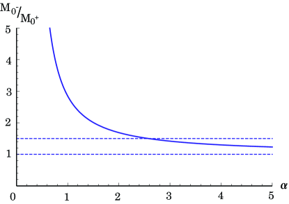
Figure 1: The mass ratio between the scalar $(M_{0^{+}})$ and pseudoscalar ($M_{0^{-}})$ glueball masses is shown as a function of the QCD running coupling $\alpha_{\rm QCD}=g_{R}(\mu)^{2}/(4\pi)$. The dotted lines represent the ratio 1 and 1.5, respectively.

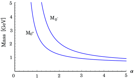
Figure 2: The scalar glueball mass $(M_{0^{+}})$ and the pseudoscalar glueball mass ($M_{0^{-}})$ are shown as a function of the QCD running coupling $\alpha_{\rm QCD}=g_{R}(\mu)^{2}/(4\pi)$. The QCD scale parameter is taken as $\Lambda_{\rm QCD}=0.20$ GeV.

In Fig.1, the mass ratio is shown as a function of the QCD coupling $\alpha_{\rm QCD}=g_{R}(\mu)^{2}/(4\pi)$. The glueball masses themselves are shown in Fig.2 as a function of $\alpha_{\rm QCD}$. Here, the QCD scale parameter is adopted as $\Lambda_{\rm QCD}=0.20$ GeV. For example, if the QCD coupling $\alpha_{\rm QCD}$ is roughly taken as $\alpha_{\rm QCD}=1.6$, then the glueball masses are obtained as

$$M_{0^{+}}=1.50\ {\rm GeV}\ ,\qquad M_{0^{-}}=2.88\ {\rm GeV}\ .$$ (160)

We cannot compare these values with experimental meson masses directly because the glueball must mix the scalar or pseudoscalar $q{\bar{q}}$-mesons, while there exist glueball candidates in particle data. So, the glueball masses obtained in our framework should be compared with the lattice QCD calculation such as $M_{0^{+}}=1.71$ GeV and $M_{0^{-}}=2.56$ GeV.[17] Further, if we take $\Lambda_{\rm QCD}=0.25$ GeV, then, $M_{0^{+}}=1.53$ GeV and $M_{0^{-}}=2.58$ GeV for $\alpha_{\rm QCD}=2.0$ are obtained. Roughly speaking, the result in this paper is not so bad.

5 Summary and concluding remarks

The scalar and the pseudoscalar glueball masses have been investigated in the framework of the time-dependent variational method and the linear response theory. We have started with the Hamiltonian of the $su(3)$ Yang-Mills gauge theory without fermions, namely QCD Hamiltonian without quarks. The time-dependent variational method within the Gaussian wavefunctional, which includes the mean field and quantum fluctuations around it, has been formulated in order to evaluate the glueball mass. The glueball mass has been calculated as the pole mass of the propagator of glueball. Here, the glueball propagator has been derived from the response with respect to the external composite field representing the glueball, which consists of two massless gluons.

The gluon mass itself is zero in this method. Thus, it is shown that the finite glueball mass is properly generated through the interaction between massless gluons. Further, since the dependence of the glueball masses on the QCD coupling constant $g$ reveals the form $1/g^{2}$, the results may not be arrived by the perturbation theory with respect to $g$.

In this paper, the coupling dependence of glueball masses was given. In the renormalization group calculation, the glueball masses $m_{G}$ are expressed as

$$m_{G}=c_{G}\mu\exp\left(\int\frac{dg}{\beta(g)}\right)=c_{G}\Lambda_{\rm QCD}\ ,$$ (161)

where $c_{G}$ is a constant.[20] Further, the similar expression was obtained in the context of the asymptotic limit in the lattice gauge theory.[21] In the strong coupling expansion of the lattice QCD, it was obtained that the glueball masses decrease when the coupling $g$ decreases,[21] while the change of mass ratio between $0^{+}$ state and $1^{+}$ or $2^{+}$ state, instead of $0^{-}$ state, is similar to our result, namely the mass ratio increases when $g$ decreases.[22] Further, in the large $N_{c}$ limit in the gauge/string duality, it seems that there is a tendency that the glueball masses decrease as $g$ decreases.[23] These results seem to be different from our result in which the glueball masses increase when $g$ decreases. However, it may be natural that, in our result, the glueball masses become very large in the asymptotic region with very small $g$, namely in the quark-gluon phase, because it may be impossible that the glueballs are excited and produced in the deconfined phase. The investigation of the implication to the strong coupling expansion or gauge/string duality is an interesting future problem.

Experimentally, it is difficult to extract the glueball masses properly because the glueball states mix the other $(q{\bar{q}})$-meson states with same quantum numbers. Thus, the glueball masses are not fixed at present. The glueball masses obtained here have been compared with the results obtained by the lattice QCD simulation. The reasonable results are included under a certain strength of QCD coupling constant. However, it should be necessary to investigate other glueball states such as $2^{+}$ state. In addition to the glueballs with the other quantum numbers, it is interesting to study the excited glueball states. In order to calculate the excited glueball masses, the other trial states $|{\Phi^{\prime}}\rangle$ may be introduced in which $\langle\Phi^{\prime}|{\Phi}\rangle=0$ should be satisfied. This treatment is similar to that of the Hartree-Fock method to calculate the excited states in the nuclear many-body problem. Another possibility is to consider the three gluon states,[24] where the external source term consists of three gluons. These investigations rest future problems. Further, in this paper, the glueball masses at zero temperature were considered because $f_{n}$ is adopted as $1/2$ in Eq.(29) or (2.1). However, if the eigenvalue of the reduced density matrix is calculated in the finite temperature $T$ in which $f_{\bf k}^{\sigma}=\sigma\cdot(n_{\bf k}^{\sigma}+1/2)$ is obtained where $n_{\bf k}^{\sigma}=1/(e^{\sigma E_{\bf k}/T}-1)$ is the bose distribution function, then, it may be possible to evaluate the glueball masses at finite temperature. These are future problems.

Appendix A Evaluation of the polarization tensor $\Pi_{0}(\omega,{\mib q})$ in the dimensional regularization scheme

Let us show the polarization tensor in Eq.(154) again:

$$\Pi_{0}(\omega,{\mib q}) \equiv g^{2}{\widetilde{\Pi}}_{0}(\omega,{\mib q})$$ (162)

$$= g^{2}\int\frac{d^{3}{\mib k}}{(2\pi)^{3}}\frac{1}{4E_{\bf k}E_{{\bf k}-{\bf q}}}\left[\frac{1}{\omega-(E_{\bf k}+E_{{\bf k}-{\bf q}})}-\frac{1}{\omega+(E_{\bf k}+E_{{\bf k}-{\bf q}})}\right]$$

$$= g^{2}\int\frac{d^{4}k}{i(2\pi)^{4}}S_{k}S_{k-q}\ ,$$

$$S_{k} = \frac{-i}{k^{2}+i\epsilon}\ .$$

Here, the 4-momentum integration is rewritten in the following form by using the Feynman parameter formula:

$$\Pi_{0}(\omega,{\mib q}) = -g^{2}\int\frac{d^{4}k}{i(2\pi)^{4}}\frac{1}{k^{2}+i\epsilon}\frac{1}{(k-q)^{2}+i\epsilon}$$ (163)

$$= -g^{2}\int_{0}^{1}dx\int\frac{d^{4}k}{i(2\pi)^{4}}\frac{1}{\left[(k-q)^{2}x+k^{2}(1-x)\right]^{2}}\ .$$

The integration of the right-hand side diverges. Thus, one needs to regularize the divergent integral to get the finite result. In this paper, the dimensional regularization method is applied and so-called modified minimal subtraction (${\overline{\rm MS}}$) scheme is adopted with the consistency to the evaluation of the QCD running coupling constant $g_{R}^{2}$.[10] Thus, the integration is regarded as the $n$-dimensional integration and is calculated as

$$\Pi_{0}(\omega,{\mib q}) = -g^{2}\int_{0}^{1}dx\int\frac{d^{n}k}{i(2\pi)^{n}}\frac{1}{\left[(k-q)^{2}x+k^{2}(1-x)\right]^{2}}$$

$$= -\frac{g^{2}\Gamma(2-n/2)}{(4\pi)^{n/2}}\int_{0}^{1}dx\frac{1}{\left[q^{2}x(x-1)\right]^{2-n/2}}$$

$$= -g^{2}(\mu^{2})^{-(2-\frac{n}{2})}\cdot(-1)^{-(2-\frac{n}{2})}\cdot\frac{\Gamma(2-n/2)}{(4\pi)^{n/2}}$$

$$\qquad\times\int_{0}^{1}dx\frac{(\mu^{2})^{2-n/2}}{(q^{2})^{2-n/2}}\cdot\frac{(-1)^{2-n/2}}{\left[x(x-1)\right]^{2-n/2}}\ ,$$

where $\Gamma(z)$ is the Gamma function. Here, we introduce a momentum scale $\mu$ to define the dimensionless coupling as follows. In $n$-dimension, QCD coupling $g$ has a dimension. Thus, the dimensionless coupling $g_{R}$ should be introduced. Then, we can further rewrite the above result as

$$\Pi_{0}(q)=-g_{R}^{2}\frac{\Gamma(\epsilon)}{(4\pi)^{2}}(-1)^{-\epsilon}\left(\frac{\mu^{2}}{q^{2}}\right)^{\epsilon}\int_{0}^{1}dx\left[\frac{4\pi}{x(1-x)}\right]^{\epsilon}\ \ ,$$ (165)

where we define the dimensionless coupling[19] as

$$g_{R}^{2}=g^{2}(\mu^{2})^{-\epsilon}\ ,$$

$$\epsilon=2-\frac{n}{2}\ .$$ (166)

Of course, if $n=4$, then $\epsilon=0$. Therefore, for infinitesimal value of $\epsilon$, we get

$$\Gamma(\epsilon) = \frac{1}{\epsilon}-\gamma+O(\epsilon)\ ,$$

$$(4\pi)^{\epsilon} = 1+\epsilon\ln 4\pi+O(\epsilon^{2})\ ,$$

$$(-1)^{-\epsilon} = 1+i\epsilon\pi+O(\epsilon^{2})\ ,$$

$$\left(\frac{\mu^{2}}{q^{2}}\right)^{\epsilon} = 1-\epsilon\ln\left(\frac{q^{2}}{\mu^{2}}\right)+O(\epsilon^{2})\ ,$$

$$\int_{0}^{1}dx\frac{1}{[x(1-x)]^{\epsilon}} = \int_{0}^{1}dx\left[1-\epsilon\ln[x(1-x)]\right]+O(\epsilon^{2})$$ (167)

$$= 1+2\epsilon+O(\epsilon^{2})\ .$$

Thus, the polarization tensor $\Pi_{0}(q)\equiv g^{2}{\widetilde{\Pi}}_{0}(q)$ can be evaluated as

$$\Pi_{0}(q) = \frac{g_{R}^{2}}{16\pi^{2}}\left[-\left(\frac{1}{\epsilon}-\gamma+\ln 4\pi\right)+\ln\frac{q^{2}}{e^{2}\mu^{2}}-i\pi+{O}(\epsilon)\right]\ .$$ (168)

Since we apply the ${\overline{\rm MS}}$-scheme in order to get a finite value by subtracting the divergent term, we subtract a part proportional to the following set:

$$\frac{1}{\overline{\epsilon}}\equiv\frac{1}{\epsilon}-\gamma+\ln 4\pi\ .$$ (169)

Finally, as a result, we get the polarization tensor as

$${\rm Re}\ \Pi_{0}(q)=\frac{g_{R}^{2}}{16\pi^{2}}\ln\frac{q^{2}}{e^{2}\mu^{2}}\ ,\qquad{\rm Im}\ \Pi_{0}(q)=-\frac{g_{R}^{2}}{16\pi}\ .$$ (170)

Appendix B Decay width

In this Appendix, the glueball mass is reconsidered by taking into account the imaginary part of the polarization tensor which may lead to the decay width of the glueball. In general, when a mass function $\Sigma(p)$ has an imaginary part, the propagator has a form

$$S_{IJ}\propto\frac{1}{p^{2}-\Sigma^{2}}=\left[p^{2}-\left(M^{2}-\frac{\Gamma^{2}}{4}\right)+iM\Gamma\right]^{-1}\ ,$$ (171)

where the mass function $\Sigma$ is divided into a real and an imaginary part as $\Sigma=M-i\Gamma/2$. Thus, the relations

$${\rm Re}\ S^{-1}(\omega,{\mib p}={\mib 0})=0\ ,$$

$${\rm Im}\ S^{-1}(\omega,{\mib p}={\mib 0})=M\Gamma$$ (172)

give the mass $M$ and $\Gamma$ that may be regarded as a decay width.

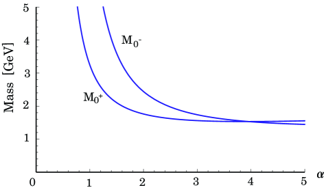
Figure 3: The scalar glueball mass $(M_{0^{+}})$ and the pseudoscalar glueball mass ($M_{0^{-}})$ are shown as a function of the QCD running coupling $\alpha_{\rm QCD}=g_{R}(\mu)^{2}/(4\pi)$, in which the imaginary part of the response function is taken into account. The QCD scale parameter is taken as $\Lambda_{\rm QCD}=0.20$ GeV.

In the treatment developed in this paper, the above relations are rewritten for the scalar $0^{+}$ and pseudoscalar $0^{-}$ glueballs as

$$1-a_{\pm}c_{3}{\rm Re}\ {\Pi}_{0}(\omega_{0^{\pm}},{\mib 0})=0\ ,\qquad\left(\omega_{0^{\pm}}^{2}=M_{0^{\pm}}^{2}-\frac{\Gamma_{0^{\pm}}^{2}}{4}\right)$$

$$-a_{\pm}c_{3}{\rm Im}\ {\Pi}_{0}(\omega_{0^{\pm}},{\mib 0})=\frac{M_{0^{\pm}}\Gamma_{0^{\pm}}}{\omega_{0^{\pm}}^{2}}$$ (173)

with $a_{+}=2$ for $0^{+}$ and $a_{-}=1$ for $0^{-}$ glueball. Here,

$$\Pi_{0}(q)\equiv g^{2}{\widetilde{\Pi}}_{0}(q)=\frac{g_{R}^{2}}{16\pi^{2}}\left(\ln\frac{q^{2}}{e^{2}\mu^{2}}-i\pi\right)\ .$$ (174)

From Eq.(B), $M$ and $\Gamma$ are obtained as

$$M_{0^{\pm}} = \frac{\mu e\cdot e^{\frac{8\pi^{2}}{3a_{\pm}g_{R}^{2}}}}{\sqrt{1-\!\left(\frac{16\pi}{3a_{\pm}g_{R}^{2}}\right)^{2}\!\left(\!\!\sqrt{1+\left(\frac{3a_{\pm}g_{R}^{2}}{16\pi}\right)^{2}}-1\!\!\right)^{2}}}$$ (175)

$$= \frac{\Lambda_{\rm QCD}\cdot\exp\left(1+\frac{\pi}{\alpha_{\rm QCD}}\left(\frac{2}{3a_{\pm}}+\frac{1}{4\pi^{2}b_{0}}\right)\right)}{\sqrt{1-\!\left(\frac{4}{3a_{\pm}\alpha_{\rm QCD}}\right)^{2}\!\left(\!\!\sqrt{1+\left(\frac{3a_{\pm}\alpha_{\rm QCD}}{4}\right)^{2}}-1\!\!\right)^{2}}}$$

$$\Gamma_{0^{\pm}} = \frac{8M_{0^{\pm}}}{3a_{\pm}\alpha_{\rm QCD}}\left(\sqrt{1+\left(\frac{3a_{\pm}\alpha_{\rm QCD}}{4}\right)^{2}}-1\right)\ .$$ (176)

In Fig.3, the glueball masses are shown as a function of $\alpha_{\rm QCD}=g_{R}^{2}/4\pi$ with $\Lambda_{\rm QCD}=0.2$ GeV. If the QCD coupling constant $\alpha_{\rm QCD}$ is roughly taken as $\alpha_{\rm QCD}=2.0$, then the glueball masses are obtained as

$$M_{0^{+}}=1.76\ {\rm GeV}\ ,\qquad M_{0^{-}}=2.44\ {\rm GeV}\ .$$ (177)

Under the above parameter set, from the imaginary part of the polarization tensor, the decay width may be evaluated, which results $\Gamma_{0^{+}}=2.54$ GeV and $\Gamma_{0^{-}}=2.61$ GeV. These values are rather large, while a large decay width is reported by using a chiral quark model.[18] As is mentioned in §4, only gluons are contained in this framework. Then, it is only possible that the glueball decays to color-octet gluons, which should be forbidden due to the color confinement. However, in our treatment, the color confinement is not considered explicitly, so the glueballs easily decay to gluons. Thus, the rather large decay width, which means a decay from the color-singlet glueball to the color-octet gluons, may be obtained unavoidably. Thus, the investigation of the decay of glueball is still remained as an open question.

Appendix C Gluon mass

In this appendix, we show that the gluon mass itself is zero in the framework developed in this paper under the Gaussian approximation used there. First, the canonical equations of motion for ${\overline{A}}_{i}^{a}({\mib x},t)$ and ${\overline{E}}_{i}^{a}({\mib x},t)$ in Eq.(9a) with (7) are given as

$${\dot{\overline{A}}}_{i}^{a}(x) = {\overline{E}}_{i}^{a}(x)\ ,$$

$${\ddot{\overline{A}}}_{i}^{a}(x) = {\dot{\overline{E}}}_{i}^{a}(x)$$ (178)

$$= -\epsilon_{ijk}\partial_{j}{\overline{B}}_{k}^{a}(x)+g\epsilon_{ijk}f^{abc}{\overline{B}}_{j}^{b}(x){\overline{A}}_{k}^{c}(x)-\frac{1}{2}\int d^{3}{\mib y}\frac{{\delta K}_{jl}^{bc}({\mib y})}{\delta{\overline{A}}_{i}^{a}({\mib x},t)}G_{lj}^{cb}({\mib y},{\mib y}),\ \quad$$

where we define

$$\frac{{\delta K}_{jl}^{bc}({\mib y})}{\delta{\overline{A}}_{i}^{a}({\mib x},t)} = -g\epsilon_{ijm}\epsilon_{mlk}f^{abd}\delta^{3}({\mib x}-{\mib y})\left(\delta_{dc}\partial_{k}^{\bf y}-gf^{dce}{\overline{A}}_{k}^{e}({\mib y},t)\right)$$ (179)

$$-g\epsilon_{lim}\epsilon_{mjk}f^{cad}\left(-\delta_{db}\partial_{k}^{\bf y}-gf^{dbe}{\overline{A}}_{k}^{e}({\mib y},t)\right)\delta^{3}({\mib x}-{\mib y})$$

$$-g\epsilon_{jlm}\epsilon_{mik}f^{bcd}\left(-\delta_{da}\partial_{k}^{\bf y}-gf^{dae}{\overline{A}}_{k}^{e}({\mib y},t)\right)\delta^{3}({\mib x}-{\mib y})\ .$$

In order to get the gluon propagator, we have to introduce the external term $H_{\rm ext}$ in the Hamiltonian as

$$H_{\rm ext}=\int d^{3}{\mib x}J_{i}^{a}({\mib x},t){A}_{i}^{a}({\mib x})=J_{i}^{a}e^{-i\omega t}\int d^{3}{\mib x}e^{i{\bf q}\cdot{\mib x}}A_{i}^{a}({\mib x})\ .$$ (180)

Thus, the gluon propagator $S_{ij}^{ab}$ can be derived by $\delta\langle A_{i}^{a}\rangle/\delta J_{j}^{b}$ following the general discussion.

Let us start with solutions ${\overline{A}}_{i}^{a}({\mib x},t)={\overline{E}}_{i}^{a}({\mib x},t)=0$ under the Hamiltonian $H_{0}$. With the external term, the solutions should be shifted. Here, we denote them as

$${\overline{A}}_{i}^{a}({\mib x},t)=0+\delta{\overline{A}}_{i}^{a}({\mib x},t)\ ,\qquad{\dot{\overline{E}}}_{i}^{a}({\mib x},t)=-\frac{\delta\langle H\rangle}{\delta{\overline{A}}_{i}^{a}({\mib x})}=-J_{i}^{a}({\mib x})\ .$$ (181)

From the equation of motion in (C), we can get the equation of motion for $\delta{\overline{A}}_{i}^{a}({\mib x},t)$ with a linear approximation for $\delta{\overline{A}}_{i}^{a}({\mib x},t)$ under small source current $J_{i}^{a}$:

$$\left((\partial_{t}^{2}-{\mib\nabla}^{2})\delta_{ij}+\partial_{i}\partial_{j}\right)\delta{\overline{A}}_{j}^{a}({\mib x},t)-\frac{c_{3}}{2}g^{2}(\delta_{il}\delta_{jk}-2\delta_{ik}\delta_{jl}+\delta_{ij}\delta_{kl})G_{lj}({\mib x})\delta{\overline{A}}_{k}^{a}({\mib x},t)$$ (182)

$$= -J_{i}^{a}({\mib x})\ ,$$

where we introduced a new notation $G_{lj}({\mib x})$ through $G_{lj}^{ab}({\mib x},{\mib x})\equiv\delta_{ab}G_{lj}({\mib x})$. In the above equation of motion, the second term, $G_{lj}({\mib x})$, is diagrammatically represented by so-called tadpole diagram. It is well known that there is no tadpole contribution in pure Yang-Mills gauge theory in the dimensional regularization scheme, namely,

$$G_{lj}({\mib x}) \propto \int\frac{d^{3}{\mib k}}{(2\pi)^{3}}\frac{1}{2|{\mib k}|}=\int\frac{d^{4}k}{i(2\pi)^{4}}\frac{-1}{k_{0}^{2}-|{\mib k}|^{2}+i\epsilon}$$ (183)

$$\rightarrow \left.\int\frac{d^{n}k}{i(2\pi)^{n}}\frac{1}{m^{2}-k^{2}}\right|_{m^{2}\rightarrow 0}$$

$$= \left.\frac{1}{(4\pi)^{\frac{n}{2}}}\frac{\Gamma(\varepsilon)}{1-\frac{n}{2}}m^{2}(m^{2}-i\epsilon)^{-\varepsilon}\right|_{m^{2}\rightarrow 0}$$

$$= -\left.\frac{1}{(4\pi)^{2}}\left[\left(\frac{1}{\varepsilon}-\gamma\right)m^{2}-m^{2}\ln m^{2}+O(\varepsilon)\right]\right|_{m^{2}\rightarrow 0}$$

$$= 0\ .$$

Thus, from the equation of motion in Eq.(182), the following equation in the momentum space is obtained:

$$\left[\omega^{2}\delta_{ij}-|{\mib q}|^{2}\left(\delta_{ij}-\frac{q_{i}q_{j}}{|{\mib q}|^{2}}\right)\right]\delta{\overline{A}}_{j}^{a}=J_{i}^{a}\ .$$ (184)

Finally, the gluon mass is given by the pole of the gluon propagator $S_{ij}^{ab}(\omega,{\mib q})={\delta{\overline{A}}_{i}^{a}}/{J_{j}^{b}}$, namely, gluon mass is exactly zero in this framework.

References

• [1] See, for example, K. Fukushima and T. Hatsuda, Rep. Prog. Phys. 74 (2011), 014001.
• [2] T. Nakano, et al., Phys. Rev. Lett. 91 (2003), 012002.
• [3] D. J. Gross and F. Wilczek, Phys. Rev. Lett. 30 (1973), 1343.
H. D. Politzer, Phys. Rev. Lett. 30 (1973), 1346.
• [4] V. Mathieu, N. Kochelev and V. Vento, Int. J. Mod. Phys. E 18 (2009), 1.
• [5] V. Crede and C. A. Meyer, Prog. Part. Nucl. Phys. 63 (2009), 74.
• [6] Y. Tsue, T.-G. Lee and H. Ishii, Prog. Theor. Phys. 122 (2009), 116.
• [7] D. Vautherin, Many-Body Methods at Finite Temperature, Advances in Nuclear Physics, Vol. 22 (Plenum Press, New York, 1996), Chap. 4.
• [8] Y. Tsue, D. Vautherin and T. Matsui, Phys. Rev. D 61 (2000), 076006.
• [9] Y. Tsue and K. Matsuda, Prog. Theor. Phys. 121 (2009), 577.
• [10] C. Heinemann, E. Iancu, C. Martin and D. Vautherin, Phys. Rev. D 61 (2000), 116008.
• [11] A. Kerman and D. Vautherin, Ann. Phys. 192 (1989), 408.
• [12] T. D. Lee, Particle Physics and Introduction to Field Theory, Reprinted by Routledge, London (2003).
• [13] R. Jackiw and A. Kerman, Phys. Lett. 71A (1979), 158.
O. Γ‰boli, R. Jackiw and S.-Y. Pi, Phys. Rev. D 37 (1988), 3557.
R. Jackiw, Physica A 158 (1989), 269.
• [14] Y. Tsue and Y. Fujiwara, Prog. Theor. Phys. 86 (1991), 443: ibid 86 (1991), 469.
• [15] T. Marumori, T. Maskawa, F. Sakata and A. Kuriyama, Prog. Theor. Phys. 64 (1980), 1294.
M. Yamamura and A. Kuriyama, Prog. Theor. Phys. Suppl. No.93 (1987), 1.
• [16] Y. Tsue, D. Vautherin and T. Matsui, Prog. Theor. Phys. 102 (1999), 313.
• [17] Y.Chen et al., Phys. Rev. D 73 (2006), 014516.
• [18] M. K. Volkov and V. L. Yudichev, Phys. Atomic Nuclei 64 (2001), 2006.
• [19] T. Muta, Foundations of Quantum Chromodynamics, World Scientific, Singapore, (1998).
• [20] G. B. West, Nucl. Phys. B 54A (1997), 353.
• [21] G. MΓΌnster, Nucl. Phys. B 190 (1981), 439.
• [22] J. Smit, Nucl. Phys. B 206 (1982), 309.
• [23] D. J. Gross and H. Ooguri, Phys. Rev. D 58 (1998), 106002.
C. CsΓ‘ki, H. Ooguri, Y. Oz and J. Terning, JHEP 01 (1997), 017.
• [24] R. L. Jaffe, K. Johnson and Z. Ryzak, Ann. of Phys. 168 (1986), 344.