Evolution of magnetic protection in potentially habitable terrestrial planets

Abstract

We present here a comprehensive model for the evolution of the magnetic properties of habitable terrestrial planets (Earth-like planets, $M\sim 1\,M_{\oplus}$ and super-Earths $M\sim\,1-10\,M_{\oplus}$) and their effects on the long-term protection against the atmospheric erosive action of stellar wind. Using up-to-date thermal evolution models and dynamo scaling laws we predict the evolution of the planetary dipole moment as a function of planetary mass and rotation rate. Combining these results with models for the evolution of the stellar wind, stellar XUV fluxes and exosphere properties of highly irradiated planets, we determine the properties of the planetary magnetosphere and the expected scale height of the atmosphere that together determine the level of thermal and non-thermal atmospheric mass losses. We have used this model to evaluate the early magnetic protection of the Earth and the already discovered potentially habitable super-Earths GJ 667Cc, Gl 581d and HD 85512b. We confirm that Earth-like planets, even under the highest attainable dynamo-generated magnetic field strengths, will lose a significant fraction of their atmospheres or their content of critical volatiles (e.g. H₂O) if they are tidally locked in the HZ of dM stars. Planets in this mass-range with N/O-rich atmospheres, even under the best conditions of magnetic protection, will probably lose their atmospheres or their water content if they are in habitable zones closer than $\sim$ 0.8 AU ($M_{\star}\lesssim 0.7-0.9M_{\odot}$). Super-Earths $M_{p}\gtrsim 3M_{\oplus}$ seem to have better chances of preserving their atmospheres even if they are tidally locked around dM stars. Under similar conditions of thermal and magnetic field evolution there seems to exist a planetary mass-dependent inner limit inside the HZ itself, below which large atmospheric mass-losses in super-Earths are expected. With the nominal value of the physical parameters in our conservative model this limit is, for example, $\sim$0.1 AU for $4M_{\oplus}$ and $\sim$0.04 AU for $8M_{\oplus}$. Under these conditions we predict that the atmosphere of GJ 667Cc has probably already been obliterated and it is presently uninhabitable. On the other hand, our model predicts that the atmospheres of Gl 581d and HD 85512b would be well protected by dynamo-generated magnetic fields even under the worst expected conditions of stellar aggression.

1. Introduction

The discovery of extrasolar habitable planets is one of the most ambitious challenges in the exoplanetary research. At the time of writing, there are almost 760 confirmed exoplanets including 55 classified as Earth-like planets (EPs, $M\sim 1\,M_{\oplus}$) and super-Earths (SEs, $M\sim\,1-10\,M_{\oplus}$, Valencia et al. 2006). Although the composition of most of these planets is unknown, many of them should have similar compositions to the Earth which would make them the first extrasolar terrestrial planets (TPs) discovered so far.

Among these low mass planets already discovered there are three confirmed SEs, GJ 667Cc, Gl 581d and HD 85512b (Selsis et al. 2007; Pepe et al. 2011; Kaltenegger et al. 2011) and tens of Kepler candidates (Borucki et al. 2011; Batalha et al. 2012) that are close or inside the habitable zone (HZ) of their host stars If we include the possibility that extra-solar-system giant planets could harbour habitable exomoons, the number of already discovered potentially habitable planetary environments beyond the Solar System could be rised to several tens (Kaltenegger 2010; Underwood et al. 2003). Moreover, the case for the existence of a plethora of other TPs and exomoons in the Galaxy is rapidly gaining evidence (Borucki et al. 2011; Catanzarite & Shao 2011; Kipping et al. 2012) and the chances that a large number of potentially habitable extrasolar bodies could be discovered in the near future are encouraging.

The question of which properties a planetary environment needs in order to allow the appearance, evolution and diversification of life has been extensively studied (for recent reviews see Lammer et al. 2009 and Kasting 2010). Two basic and complimentary physical conditions must be fulfilled: the presence of an atmosphere and the existence of surface liquid water (Kasting et al. 1993). However, the fulfilment of these basic conditions depends on many complex and diverse endogenous and exogenous factors (for a comprehensive enumeration of these factors see e.g. Ward & Brownlee 2000 or Lammer et al. 2010)

The existence and long-term stability of an intense planetary magnetic field (PMF) is one of these additional factors (see e.g. Grießmeier et al. 2010 and references therein). It has been shown that a strong enough PMF would protect the atmosphere of potentially habitable planets, especially its valuable content of water and other volatiles, against the erosive action of the stellar wind (Lammer et al. 2003, 2007; Khodachenko et al. 2007; Chaufray et al. 2007). Planetary magnetospheres would also act as shields against the potentially harmful effects that the stellar and galactic cosmic rays (CR) could produce in the life-forms evolving on its surface (see e.g. Grießmeier et al. 2005). Even in the case that life could arise and evolve on unmagnetized planets, the detection of atmospheric biosignatures would be also affected by a higher flux of stellar and galactic CR, especially if the planet is around very active M-dwarfs (dM) (Grenfell et al. 2007; Segura et al. 2010). In summary, a PMF would not only protect the atmosphere of the planet and the life growing on its surface, but also give us the possibility to confirm the habitability of future discovered planets around dM stars.

But find suitable conditions to have TPs with strong enough PMFs in the HZ of the most abundant stars seems more problematic than previously thought. It has been recently predicted that most of the TPs in our Galaxy could be found around dM stars (Boss 2006; Mayor & Udry 2008; Scalo et al. 2007; Rauer et al. 2011). Actually $\sim 20\%$ of the presently confirmed super-Earths belong to planetary systems around stars of this type, including Gl 581d one of the best candidate for habitability presently known (Selsis et al. 2007). Planets inside the HZ of low mass stars ($M_{\star}\lesssim 0.6M_{\odot}$) would be tidally locked (Joshi et al. 1997; Heller et al. 2011) a condition that poses serious limitations to their potential habitability (see e.g. Kite et al. 2011 and references therein). Tidally locked planets inside the HZ of dMs will have periods in the range of $5-100$ days, a condition has commonly been associated with the almost complete lack of a protective magnetic field (Grießmeier et al. 2004). However, the relation between rotation and PMF properties, that is critical to assess the magnetic protection of slowly rotating planets, is more complex than previously thought (Zuluaga & Cuartas 2012). In particular a detailed knowledge of the thermal evolution of the planet is required to predict not only the intensity but also the regime (dipolar or multipolar) of the PMF for a given planetary mass and rotation rate.

Several authors have extensively studied the protection that intrinsic PMF would provide to extrasolar planets (Grießmeier et al. 2005; Khodachenko et al. 2007; Lammer et al. 2007; Grießmeier et al. 2009, 2010). Independently the effects of X-Ray and EUV radiation (XUV) on the thermal escape processes in weakly magnetized planets have also been studied (Kulikov et al. 2006; Lammer et al. 2007, 2009; Tian et al. 2008; Tian 2009; Sanz-Forcada et al. 2010). All these works have however neglected the evolving nature of the PMF and have systematically predicted field intensities using scaling-laws that have been revised in the last couple of years (see Christensen 2010 and references therein). More importantly the role of rotation in determining the PMF properties that is critical in assessing the case of tidally locked planets has been overlooked (Zuluaga & Cuartas 2012).

In this work we present a model of the evolution of the magnetic protection of potentially habitable TPs around GKM main sequence stars. To achieve this goal we integrate in a single framework the most recent thermal evolution models for this type of planets (Gaidos et al. 2010; Tachinami et al. 2011), up-to-date dynamo scaling-laws (Christensen 2010; Zuluaga & Cuartas 2012), models for the evolution of the stellar wind and XUV luminosity of low mass-stars (Grießmeier et al. 2010; Sanz-Forcada et al. 2011) and the most recent results describing the expansion and hydrodynamical escape of volatiles from highly irradiated atmospheres of low mass planets (Kulikov et al. 2006; Tian et al. 2008; Tian 2009). This is the first time that all these pieces have been put together to produce a global picture of the magnetic protection of potentially habitable TPs.

But this is not only a model integration effort. Several novel features have been added to our comprehensive model: 1) we include a new treatment of the role of rotation in determining the PMF properties, eespecially important in assessing the magnetic protection of tidally locked planets, 2) we propose a phenomenological formula to estimate a magnetic-constrained thermal mass-loss rate from atmospheres protected with a strong PMF, and 3) we address the magnetic protection of already discovered habitable planets and compare it with the case of an early magnetized Venus and the Earth in its current state.

This paper is organized as follows: section 2 describes the model used here to calculate the evolution of magnetosphere properties. For that purpose we use a set of analytical fits of recently published models for the thermal evolution of TPs (section 2.1) and up-to-date power-based dynamo scaling laws (section 2.2). Several stellar key properties are required to calculate the evolution of the magnetopshere (stellar wind properties, HZ distances and tidally locking limits). The way we obtain these properties and their evolution are described in section 2.3. Atmospheric expansion models and the proposed phenomenological formula to model the atmospheric mass-loss rate are described in section 3. Section 4 presents the results of applying this model to hypothetical and already discovered habitable TPs. A discussion about the hypothesis on which the model relies and the possible sources of uncertainties are presented in section 5. Finally several conclusions and the future prospects of this work are summarized in section 6.

2. A model for an evolving magnetosphere

The interaction between the PMF, the interplanetary magnetic field (IMF) and the stellar wind creates a magnetic cavity around the planet known as the magnetosphere. Magnetospheres are very complex systems but its basic properties are continuous functions of two basic variables (Siscoe & Christopher 1975): the planetary magnetic dipole moment ${\cal M}$ and the dynamical pressure of the stellar wind $P_{\rm sw}$:

$${\cal M}=\frac{4\pi r^{3}B_{p}^{\rm dip}(r)}{\sqrt{2}\mu_{0}},$$ (1)

$$P_{\rm sw}=mnv_{\rm eff}^{2}+2nk_{B}T.$$ (2)

Here $B_{p}^{\rm dip}(r)$ is the dipolar component of the field as measured at distance $r$ from the planet center. $m$ and $n$ are the typical mass of a wind particle (mostly protons) and its number density, respectively. $v_{\rm eff}=(v_{\rm sw}^{2}+v_{p}^{2})^{1/2}$ is the effective average velocity of the stellar wind as measured in the reference frame of the planet whose orbital velocity is $v_{p}$. And $T$ is the local temperature of the plasma. $\mu_{0}=4\pi\times 10^{-7}\,\rm{H/m}$ and $k_{B}$ are the vacuum permeability and Boltzmann constant respectively.

There are three basic properties of planetary magnetospheres we are interested in: 1) the maximum magnetopause field intensity $B_{mp}$, a proxy to the flux of high energy particles into the magnetospheric cavity, 2) the standoff or stagnation radius, $R_{S}$, a measure of the size of the dayside magnetosphere, and 3) the area of the polar cap $A_{pc}$ that measures the total area of the planetary atmosphere exposed to open field lines through which particles can escape to interplanetary space. The value of these three quantities provides information about the level of exposure that a habitable planet has to the erosive effects of stellar wind and the potentially harmful effects of the CR.

The maximum value of the magnetopause field intensity $B_{\rm mp}$ is estimated by equating the magnetic pressure $P_{\rm mp}=B_{\rm mp}^{2}/(2\mu_{0})$ and the dynamical stellar wind pressure $P_{\rm sw}$ (eq. 2),

$$B_{\rm mp}=(2\mu_{0})^{1/2}P_{\rm sw}^{1/2}$$ (3)

Although the magnetopause fields arise from very complex processes (Chapman-Ferraro and other currents at the magnetosphere boundary), in simplified models $B_{\rm mp}$ is parametrized as a multiple of the planetary field intensity $B_{\rm p}$ as measured at the substellar point $r=R_{S}$ (Mead 1964; Voigt 1995),

$$B_{\rm mp}=2f_{0}B_{\rm p}(r=R_{S})=\left(\frac{f_{0}\mu_{0}}{2\pi}\right)\sqrt{2}{\cal M}R_{S}^{-3}$$ (4)

where $f_{0}$ is a numerical enhancement factor of order 1. We are assuming here that the dipolar component of the intrinsic field dominates at magnetopause distances even in slightly dipolar PMF. Combining equation 3 and 4 we obtain an estimate of the standoff distance:

$$R_{S}=\left(\frac{\mu_{0}f_{0}^{2}}{8\pi^{2}}\right)^{1/6}\mathcal{M}^{1/3}P_{\rm sw}^{-1/6}$$ (5)

It is important to stress here that the $R_{S}$ given by eq. (5) assumes that the pressure exerted by the gasses trapped inside the magentosphere cavity is negligible. This is a good approximation only if the planetary magnetic field is very intense or the stellar wind is weak or the planetary atmosphere is not too bloated by the XUV radiation. In the case when any or none of these condition are fulfilled we will refer to the $R_{S}$ estimated with eq. (5) as the magnetic standoff distance.

The last but not least important property in which we are interested is the area of the polar cap. The polar cap is the region in the magnetosphere where open field lines could transport ions into or from the interplanetary space. Siscoe & Chen (1975) showed that the area of the polar cap $A_{\rm pc}$ scales with the dipole moment and the dynamical pressure of the stellar wind as:

$$A_{\rm pc}=4.63\times 10^{-2}\left(\frac{\cal M}{{\cal M}_{\oplus}}\right)^{-1/3}\left(\frac{P_{\rm sw}}{P_{\rm sw\odot}}\right)^{1/6}$$ (6)

where ${\cal M}_{\oplus}=7.768\times 10^{22}\,\rm{Am}^{2}$ and $P_{\rm sw\odot}=2.24\,\rm{nPa}$ are the present values of the dipole moment of the Earth and the average dynamic pressure of the solar wind as measured at the Earth distance (Stacey 1992; Grießmeier et al. 2005).

In order to model the evolution of the magnetosphere properties we need to calculate reliable values of the surface dipolar component of the PMF $B_{\rm p}^{dip}$, the average number density $n$, the velocity $v_{\rm eff}$ and the temperature $T$ of the stellar wind. These quantities depend in general on time and also on different planetary and stellar properties. In the following sections we describe the models used in this work to calculate the evolving values of these critical quantities.

2.1. Planetary thermal evolution

We assume here that the main source of a global PMFs in TPs is the action of a dynamo powered by convection in a liquid iron core. Other possible sources of PMFs, dynamo action in a mantle of ice, water or magma or stellar induced magnetic fields, are not considered here.

The properties and evolution of a core dynamo will depend on the internal structure and thermal history of the planet. Two recent works have built and solved detailed interior and thermal evolution models intended to study the generation of intrinsic PMF in super Earths (Gaidos et al. 2010; Tachinami et al. 2011) . These works have paid attention to different and complimentary aspects of the problem: while Gaidos et al. (2010) have concentrated on the thermodynamics of the core, Tachinami et al. (2011) have developed a detailed treatment of mantle rheology and convection. From these works a robust picture of the thermal evolution of SEs is starting to arise. More recently Zuluaga & Cuartas (2012) have shown how by combining the results of these thermal evolution models and the rotational properties of the planets it is possible to predict not only the mean intensity of the magnetic field, but also its regime (dipolar or multipolar). This last property is important in predicting the intensity of the dipolar component of the field at the planetary surface and from there the dipole moment of the planet.

There are three key properties that should be predicted by any thermal evolution model in order to calculate the magnetic properties of the planet: 1) the total convective power $Q_{\rm conv}$ providing the energy to be dissipated through dynamo action, 2) the radius of the solid inner core $R_{\rm ic}$ and thus the height $D$ of the convecting shell where the dynamo action takes place ($D=R_{c}-R_{\rm ic}$) and 3) the total dynamo life-time $t_{\rm dyn}$. Figure 1 shows the values of these quantities as predicted by the model by Gaidos et al. (2010) for planets with the same composition as the Earth in the mass range 1.0-4.8 $M_{\oplus}$.

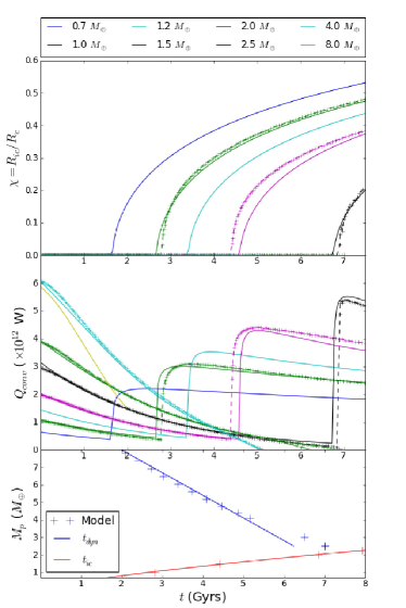
Figure 1.— Results of the thermal evolution model by Gaidos et al. (2010) for TPs with the same composition as the Earth. Upper panel, radius of the solid inner core. Middle panel, total convective power. Lower panel, time of the inner core nucleation (red) and dynamo lifetime (blue). Numerical results are indicated as crosses joined by dashed lines. Continuous lines correspond to the analytical fit used in this work to interpolate and extrapolate the model results (see text).

We have selected the model results obtained for planets with mobile lids and habitable surface temperatures $T_{\rm surf}$=288 K. We assume that the potentially habitable planets described with our magnetic protection model fulfill this condition at least for the time during which they have a dense enough atmosphere and an available inventory of water.

In this model all planets start their thermal history with a liquid iron core with radius $R_{c}$. The iron core cools down through the release of heat stored during the early phases of the formation of the planet (sensible heat) and generated by the decay of radionuclides. The contribution of tidal heat in this process has, however, been negelected. When the temperature at the center of the planet has decreased below a critical level, an inner solid core starts to form and suddenly new sources of energy arise (release of latent heat and buoyancy generated by the release of light elements). This change produces a strong “rebounce” of $Q_{\rm conv}$ after the initiation of inner core growing (see middle panel in figure 1). However, this phenomenon is restricted to planets with masses $M_{p}\lesssim M_{\rm crit}\approx 2-2.5\,M_{\oplus}$ (a threshold predicted independently by Tachinami et al. 2011). On planets with a larger mass than this limit the dynamo shuts down before the inner core starts to grow, either because iron snow is formed at the core mantle boundary (CMB) or the temperature contrast through the CMB falls below the value required to ensure convection.

The model by Gaidos et al. 2010 is restricted to a discrete set of masses between 1 and 4.8 $M_{\oplus}$. In order to interpolate the thermal evolution properties to other planetary masses we have developed analytical fits for $R_{\rm ic}$, $Q_{\rm conv}$ and $t_{\rm dyn}$. We have found that $R_{\rm ic}$ and $Q_{\rm conv}$ could be fitted using a combination of double exponential functions $f(x)\sim\exp(x^{a})$. It has been observed that other complex thermodynamic phenomena could be fitted well by double exponential functions. This could imply that our analytical fits more than having a mere practical value could also have some phenomenological roots.

The rising of $R_{\rm ic}$ for planets below the critical mass $M_{\rm crit}=2\,M_{\oplus}$ could be computed analytically using:

$$\chi(t)={\chi}_{\infty}\left(1-\exp\left[-(t-t_{\rm ic})^{1/4}\right]\right)^{3}.$$ (7)

Here $\chi_{\infty}$ is a fitting parameter that depends on planetary mass. The exponents 1/4 and 3 are found almost independently of planetary mass. We have additionally found that $\chi_{\infty}$ scales with planetary mass $M_{p}$ follow a simple power law,

$$\chi_{\infty}(M_{p})=1.008\,(M_{p}/M_{\oplus})^{-7/5},$$ (8)

where we have approximated the exponent to the nearest rational value (-7/5). Using eq. (7) and (8) we can calculate analytical approximations of the inner core radius for any planetary mass and at any given time after the inner core nucleation (solid lines in the upper panel of figure 1). As expected the combined fit of $\chi_{\infty}$ and $\chi(t)$ have some discrepancies with the numerical results. However, we have verified that most of them come from the difference between the actual value of the time of inner-core nucletion $t_{\rm ic}$ and the fitted value of this quantity (red line in the lower panel of figure 1). The observed differences, as measured on the time axis, are no larger than $0.1$ Gyr, i.e. they are below the resolution of the magnetosphere evolution model presented here.

$Q_{\rm conv}$ is more complex. We have fitted the decaying initial phase (release of sensible heat) and the rebounce phase after inner core nucleation (release of combined sensible and latent heat) independently. The resulting piecewise fitting function reads as:

$$\frac{Q_{\rm conv}}{10^{12}\,{W}}=\left\{\begin{array}[]{ll}q_{\rm Sl}\,\exp(t/t_{\rm Sl})^{1},&M<M_{\rm crit},t<t_{\rm ic}\\ q_{\rm L}\,(t-t_{\rm ic})^{1/3}\times\\ \;\;\times\exp[(t-t_{\rm ic})/t_{\rm L}]^{1/4},&M<M_{\rm crit},t>t_{\rm ic}\\ q_{\rm Sh}\,\exp[(t-t_{\rm oh})/t_{\rm Sh}]^{2},&M>M_{\rm crit},\forall\;t\end{array}\right.$$ (9)

The fitting parameters $q_{\rm Sl}$, $q_{\rm Sh}$, $q_{\rm L}$, $t_{\rm Sl}$, $t_{\rm L}$, $t_{\rm oh}$ and $t_{\rm Sh}$ scale also with planetary mass and the scaling coefficients are presented in table 1.

$x$	$\alpha_{x}$	$\beta_{x}$	Mass Range
			$M_{\oplus}$
Planetary Properties
$R_{p}$	6378 km	0.265	0.7-10
$R_{c}$	1370 km	0.243	”
$\rho_{c}$	11 g/cm3	0.271	”
$R_{\rm ic}$
$t_{\rm ic}$	2.620 Gyr	1.360	”
$\chi_{\infty}$	1.008	-0.140	”
$Q_{\rm conv}$
$q_{\rm Sl}$	1.090	1.528	0.7-$M_{\rm crit}$
$t_{\rm Sl}$	2.907 Gyr	-0.155	”
$q_{\rm L}$	13.529	1.170	”
$t_{\rm L}$	0.190 Gyr	-0.883	”
$q_{\rm Sh}$	12.616	-0.350	$M_{\rm crit}$-10
$t_{\rm oh}$	-46.096 Gyr	-2.272	”
$t_{\rm Sh}$	15.105 Gyr	-0.965	”

Table 1Scaling coefficients for planetary properties and thermal evolution fitting parameters. Property $x$ is scaled using a simple power law function $x=\alpha_{x}(M_{p}/M_{\oplus})^{\beta_{x}}$ where $\alpha_{x}$ is the reference value for $x$ (the value at $M_{p}=1\,M_{\oplus}$) and $\beta_{x}$ is the scaling exponent. $M_{\rm crit}$ is the maximum mass for planets to develop a solid inner core before the shutting down of the core dynamo.

The combination of analytical fits and power-law scaling of the fitting parameters allows us also to extrapolate the thermal evolution results to other planetary masses. Gaidos et al. 2010 used their model to study the case of planets with a larger mass than 4.8 $M_{\oplus}$ focusing on the dynamo lifetime. On the other hand, Tachinami et al. 2011 also applied their model for planets with a smaller mass than the Earth. We assume here that there are no other critical phenomena that avoid the extrapolation of the behavior observed in the reported mass-range to higher and lower planetary masses. We will model here planets in the mass range $0.7-10M_{\oplus}$.

Other application of the analytical fitting functions to the thermal evolution of TPs is that it provides a way to test the impact that different parameters of the thermal evolution have on the protective properties of the evolving PMF. We can check, for example, what would happen if an improved thermal evolution model predicted a different critical mass $M_{\rm crit}$ or different values for the time of inner core nucleation $t_{\rm ic}$. We will return to this sensitivity check in section 5.

2.2. Planetary magnetic field

In recent years improved numerical experiments have constrained the full set of possible scaling laws used to predict the properties of planetary and stellar convection-driven dynamos (see Christensen 2010 and references therein). It has been found that in a wide range of physical conditions the global properties of convection-driven dynamos can be expressed in terms of simple power-law functions of the total convective power $Q_{\rm conv}$ available for dynamo action.

One of the most important results of power-based scaling laws is the fact that the volume averaged magnetic field intensity inside the convecting shell $B_{\rm rms}^{2}=(1/V)\int B^{2}dV$ does not depend on the rotation rate (eq. 6 in Zuluaga & Cuartas 2012),

$$B_{\rm rms}\approx C_{\rm Brms}\;\mu_{0}^{1/2}{\overline{\rho}_{c}}^{1/6}(D/V)^{1/3},Q_{\rm conv}^{1/3}$$ (10)

where $C_{\rm Brms}=0.24$ for dipolar dominated dynamos and $C_{\rm Brms}=0.18$ for multipolar dynamos. $\overline{\rho}_{c}$, $D\approx R_{c}(1-\chi)$ and $V\approx 4/3\pi R_{c}^{3}(1-\chi^{3})$ are the average density, height and volume of the convective shell. We are assuming that the whole external liquid iron core is convecting. In a real case only a fraction of the core volume is involved in dynamo action and therefore the magnetic fields predicted with equation 10 and with our assumption will underestimate the actual field strenght (Gaidos, E. 2011). We have, however, verified that this effect is only important for time periods much longer than the time it takes to start the inner core nucleation. For a planet with the same mass as the Earth the time during which the stellar aggression is the largest is much less than that time for inner core nucleation (see section 4).

The dipolar field intensity at the planetary surface, and hence the dipole moment of the PMF, can be estimated if we have information about the power spectrum of the magnetic field at the core surface. Although we cannot predict the relative contribution of each mode to the total core field strength, numerical dynamos exhibit an interesting property: there is a scalable adimensional quantity, the local Rossby number $Ro^{*}_{l}$, that could be used to distinguish dipolar dominated from multipolar dynamos. The scaling relation for $Ro^{*}_{l}$ is (eq. 5 in Zuluaga & Cuartas 2012):

$$Ro^{*}_{l}=C_{\rm Rol}\;{\overline{\rho}_{c}}^{-1/6}R_{c}^{-2/3}D^{-1/3}V^{-1/2}Q_{\rm conv}^{1/2}P^{7/6}.$$ (11)

Here $C_{\rm Rol}=0.67$ is a fitting constant and $P$ is the period of rotation. It has been found that dipolar dominated fields arise systematically when dynamos have $Ro^{*}_{l}<0.1$. Multipolar fields arise in dynamos with values of the local Rossby number close to and larger than this critical value. From eq. (11) we see that in general fast rotating dynamos (low $P$) will have dipolar dominated core fields while slowly rotating ones (large $P$) will produce multipolar fields and hence fields with a much lower dipole moment.

It is important to stress that the almost independence of $B_{\rm rms}$ on rotation rate, together with the role that rotation has in the determination of the core field regime, implies that even very slowly rotating planets, for example those whose rotation is locked by the action of the tidal effect of its host star (tidally locked planets), could have a comparable magnetic energy budget to rapidly rotating planets with similar size and thermal histories. In the former case the magnetic energy will be redistributed among other multipolar modes rendering the core field more complex in space and probably also in time. Together all these facts introduce a non-trivial dependence of dipole moment on rotation rate very different than that obtained with the traditional scaling laws used by previous works (see e.g. Grießmeier et al. 2004 and Khodachenko et al. 2007).

Using the value of $B_{\rm rms}$ and $Ro^{*}_{l}$ we can compute the maximum dipolar component of the field at core surface. For this purpose we use the maximum dipolarity fraction $f_{\rm dip}$ (the ratio of the dipolar component to the total field strength at core surface) that for dipolar dominated dynamos $f_{\rm dip}^{max}\approx 1.0$ and for multipolar ones $f_{\rm dip}^{max}\approx 0.35$ (see Zuluaga & Cuartas 2012 for details). To connect this ratio to the volumetric averaged magnetic field $B_{\rm rms}$ we use the volumetric dipolarity fraction $b_{\rm dip}$ that it is found, as shown by numerical experiments, conveniently related with the maxium value of $f_{\rm dip}$ through eq. (12) in Zuluaga & Cuartas 2012,

$$b_{\rm dip}^{min}=c_{\rm bdip}{f_{\rm dip}^{max}}^{-11/10}$$ (12)

where $c_{\rm bdip}\approx 2.5$ is again a fitting constant. Finally by combining eqs. (10-12) we can compute an upper bound to the dipolar component of the field at the CMB:

$$B_{c}^{dip}\lesssim\frac{1}{b_{\rm dip}^{min}}B_{\rm rms}=\frac{{f_{\rm dip}^{max}}^{11/10}}{c_{\rm bdip}}\;B_{\rm rms}$$ (13)

The surface dipolar field strength is estimated using,

$$B_{p}^{dip}(R_{p})=B_{c}^{dip}\left(\frac{R_{p}}{R_{c}}\right)^{3}$$ (14)

and finally the total dipole moment is calculated using eq. (1) for $r=R_{p}$.

It should be emphasized that the surface magnetic field intensity determined using eq. (14) overestimates the actual PMF dipole component. The actual field could be much more complex spatially. Using our model we can only predict the maximum level of protection a given planet could have from a dynamo-generated intrinsic PMF.

We show in figure 2 the result of applying the previously described method to calculate the dipole moment for TPs. We compare them with the static value of the same quantity as computed by the rotation dependent dynamo scaling law by Sano 1993 that has been commonly used in previous works. The differences between both approaches are significant. Not only the estimated values of the dipole moment are quite different but the general dependence on planetary mass and rotation period is much more rich and complex. Those differences have important and previously unknown consequences in the magnetic protection of tidally locked and unlocked habitable planets. We will return to this point in section 4.

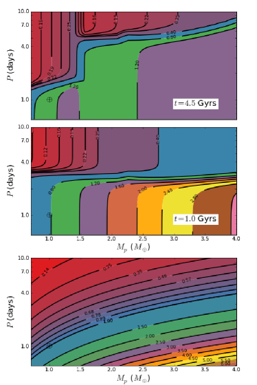
Figure 2.— Maximum dipole moment predicted with the power-based scaling laws used in this work (upper and middle panels) and the rotation dependent scaling law by Sano 1993 (lower panel).

2.3. Stellar properties

Once we have determined the PMF intensity, the other element required to estimate the magnetosphere properties is the dynamical pressure of the stellar wind. However, magnetic protection does not only depend on the size of the magnetosphere. The scale height of the atmosphere should be also estimated and compared with the magnetopause distance. Highly irradiated atmospheres, such as those of close-in planets at early phases of the stellar evolution, could be expanded enough to be exposed to the direct action of stellar wind. In this case we will therfore also need to estimate the level of high energy flux at the top of the atmopshere of our habitable planets. In this section we describe the models used in this work to calculate all the relevant properties concerning the interaction between the star and the planetary magnetosphere and atmosphere.

The properties of low-mass stars are still very uncertain (see e.g. Engle & Guinan 2011). However, since our magnetic field model is able only to determine the maximum intensity of the PMF we will only be interested in limits of the stellar properties providing the lower level of “stellar aggression” (the minimum stellar wind pressure and XUV irradiation). Combining upper bounds for the magnetic properties of the planet and lower bounds for the stellar aggression will give us an overestimation of the overall magnetic protection of the planet. In this way if, under our conservative model, a planet results endangered or unprotected, the actual case will be even worse.

2.3.1 Habitable zones and tidally locking limits

The effects a star has on the planetary environment depend on three basic factors: 1) the fundamental properties of the star, luminosity $L_{\star}$, effective temperature $T_{\rm\star}$ and radius $R_{\star}$, 2) the average distance of the planet from the star (distance to the HZ) and 3) the relation between the rotation and orbital period, in particular if they are conmensurable (tidally locked planet) or not5D (unlocked planet).

For the stellar properties we are using the results obtained by Baraffe et al. 1998 (thereafter BCAH98) who calculated the evolution of low-mass stars in a wide range of metallicities including the solar value. In all cases we assume the same metallicity for the stars as the Sun. For simplicity we are also assuming that the basic stellar properties, temperature, luminosity and radius, are constant during the range of time in which we are calculating the magnetosphere properties $t=0.7-3$ Gyr (see section 2.3.2). To be consistent with the purpose of computing the best case for magnetic protection, we take the stellar properties predicted by the model at the end of the time interval, i.e. $t=3.0$ Gyr. At that time the HZ will be placed at the greatest distance from the star especially for stars in the mass range $M_{\star}=0.8-1.0$ and therefore the stellar wind pressure and XUV irradiation will be minimum.

To determine the distance to the HZ we use here the results obtained by Kasting et al. 1993. Although the detailed atmospheric models by Kasting et al. 1993 were calculated for only three stellar masses, we use the parabolic fitting developed by Selsis et al. 2007 to calculate the inner $a_{\rm in}$ and outer edges $a_{\rm out}$ of the HZ of arbitrary GKM stars:

$$\begin{array}[]{lll}a_{\rm in}&=&(a_{in\odot}-\alpha_{\rm in}\Delta T-\beta_{\rm in}\Delta T^{2})\sqrt{L/L_{\odot}}\\ a_{\rm out}&=&(a_{out\odot}-\alpha_{\rm out}\Delta T-\beta_{\rm out}\Delta T^{2})\sqrt{L/L_{\odot}}\end{array}$$ (15)

where $a_{in\odot}$ and $a_{out\odot}$ are the inner and outer edges of the HZ for the present sun, $\Delta T=T-T_{\odot}$ and $\alpha$ and $\beta$ are fitting constants. To define our HZ we use the conservative limits given by the criteria of “recent Venus” and “early Mars” (Kasting et al. 1993). In this case $a_{in\odot}=0.72$, $\alpha_{\rm in}=2.7619\times 10^{-5}$, $\beta_{\rm in}=3.8095\times 10^{-9}$, $a_{in\odot}=1.77$, $\alpha_{\rm out}=1.3786\times 10^{-4}$, $\beta_{\rm out}=1.4286\times 10^{-9}$ (Selsis et al. 2007).

Planets at close-in orbits are affected by the tidal interaction with the host star. This interaction dampens the primordial rotation of the planets leaving them in a resonant rotational state where the period of rotation $P$ becomes commensurable with the orbital period $P_{o}$,

$$P:P_{o}=n:2$$ (16)

Where $n$ is an integer larger than or equal to 2. The value of $n$ is determined by multiple dynamical factors one the most important being the orbital eccentricity. The maximum distance $a_{\rm tid}$ at which a solid planet in a circular orbit becomes tidally locked before a given time $t$ is given by (Peale 1977),

$$a_{\rm tid}(t)=0.5\,\rm{AU}\,\left[\frac{(M_{\star}/M_{\odot})^{2}P_{\rm prim}}{Q}\right]^{1/6}t^{1/6}$$ (17)

Where the primordial period of rotation $P_{\rm prim}$ should be expressed in hours, $t$ in Gyr and $Q$ is an adimensional dissipation function. For the purposes of this work we assume the same value of the estimated primordial rotation period of the Earth for all planets, $P_{\rm prim}\approx 17\,\rm{hours}$ (Varga et al. 1998; Denis et al. 2011) and a dissipation function $Q=100$ typical for terrestrial planets.

In figure 3 we depict the value of the stellar properties, HZ and tidally locked limits for the stars in the mass-range studied in this work.

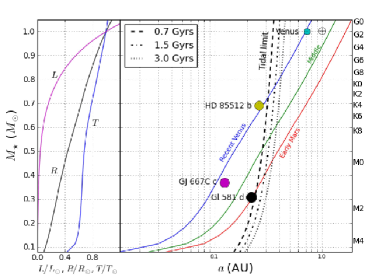
Figure 3.— Stellar properties, HZ and tidally locking limits for solar metallicity GKM stars. Stellar properties are computed from the BCAH98 model at $t=3$ Gyr. Tidally locking limits assume $P_{\rm prim}=17$ hours, and $Q=100$.

2.3.2 Stellar wind

The properties of the stellar wind change in time and vary with the distance from the host star. Dur to this dependence on distance and for the sake of simplicity we have used here the pure hydrodynamical isothermal model developed by Parker 1958 (hereafter the Parker’s model). It has been shown that this simple model reliably predicts the stellar wind properties of stars with periods of rotation of the same order as the present solar value, i.e. $P\sim 30$ days (Preusse et al. 2005). For rapidly rotating stars, i.e. young stars and/or active dM stars, the Parker’s model underestimates the stellar wind properties by a factor up to 2 (Preusse et al. 2005). Given the dependence of the magnetosphere properties on the stellar wind pressure (equations 3-6) the rotation-independent model will give us values for the magnetopause fields, standoff distances and polar cap areas, between 10-40% off the values obtained with a more detailed model (e.g. the extended model by Weber & Davis 1967). Magnetopause fields have the largest uncertainties ($\sim 40\%$) while standoff distances and polar cap areas, that as we will also shown are the most critical parameters, are off by just $\sim 10\%$ (standoff radius will be overestimated while polar cap areas are underestimated).

According to the Parker’s model the stellar wind average particle velocity $v$ at distance $d$ from the host star is obtained by solving the Parker’s wind equation:

$$u^{2}-\log u=4\log\rho+\frac{4}{\rho}-3$$ (18)

where $u=v/v_{c}$ and $\rho=d/d_{c}$ are a normalized velocity and distance and $v_{c}=\sqrt{k_{B}T/m}$ and $d_{c}=GM_{\star}m/(4k_{B}T)$ are respectively the local sound velocity and critical distance where the stellar wind becomes subsonic. In this model $T$ is the temperature of the stellar corona and appears here as the key parameter that determines the properties of the stellar wind. The number density $n$ is determined from the velocity at each distance using the continuity equation,

$$n=\frac{\dot{M_{\star}}}{4\pi d^{2}vm}$$ (19)

The time dependence of the stellar wind properties is much harder to estimate. We have used here the formulas derived by Grießmeier et al. 2004 and Lammer et al. 2004 and that were originally based on the observational estimates of the stellar mass-loss rate by Wood et al. 2002 and the theoretical evolution models by Newkirk 1980. For main-sequence stars and times $t>0.7$ Gyr, the long-term averaged stellar wind velocity and number density as measured at a distance of 1 AU is estimated by:

$$v_{1\rm{AU}}(t)=v_{0}\left(1+\frac{t}{\tau}\right)^{\alpha_{v}}$$ (20)

$$n_{1\rm{AU}}(t)=n_{0}\left(1+\frac{t}{\tau}\right)^{\alpha_{n}}$$ (21)

Where $\alpha_{v}=-0.43$, $\alpha_{n}=-1.86\pm 0.6$ and $\tau=25.6\,\rm{Myr}$ (Grießmeier et al. 2009). $v_{0}=3971$ km/s and $n_{0}=1.04\times 10^{11}\,\rm{m}^{-3}$ were estimated assuming present long-term averages of the solar wind as measured at the distance of the Earth, i.e. $n(4.6\,\rm{Gyr},1\,M_{\odot},1\,\rm{AU})=6.59\times 10^{6}\,\rm{m}^{-3}$ and $v(4.6\,\rm{Gyr},1\,M_{\odot},1\,\rm{AU})=425\,\rm{km/s}$ (Schwenn 1990). For times $t<0.7$ Gyr stellar wind models are too uncertain and the estimates provided by eqs. (20) and (21) become unreliable (Wood et al. 2002).

Grießmeier et al. 2007 devised a clever way to combine the distance dependent estimation of the stellar wind properties, given for example by the Parker’s model, with the time variation of the reference number density and velocity given by eqs. (20) and (21). For the sake of completeness in this work we summarize the procedure by Grießmeier et al. 2007 but for further details we refer to section 2.4 of that work.

The stellar wind properties at time $t$ and distance $d$ for a given stellar mass are calculated by estimating first the coronal temperature $T(t)$ for which the velocity obtained with the Parker’s equation evaluated at $d=1$ AU coincides with the reference velocity obtained by eq. (20) evaluated at time t. Using the coronal temperature $T(t)$ the Parker’s equation provides the velocity at any distance from the star at that time. The number density is obtained from the continuity equation (19) assuming that the stellar mass-loss rate scales with the stellar radius as $\dot{M}_{\star}(t)=\dot{M}_{\odot}(t)(R_{\star}/R_{\odot})^{2}$, where the solar reference mass-loss rate $\dot{M}_{\odot}$ is computed using:

$$\dot{M}_{\odot}(t)=4\pi(1\,\rm AU)^{2}\;m\;n_{1\rm{AU}}(t)v_{1\rm{AU}}(t)$$ (22)

The values of the stellar wind dynamical pressure $P_{\rm dyn}=mnv^{2}$ inside the HZ of four different stars as computed using the procedure described before are plotted in the upper panel of figure 4.

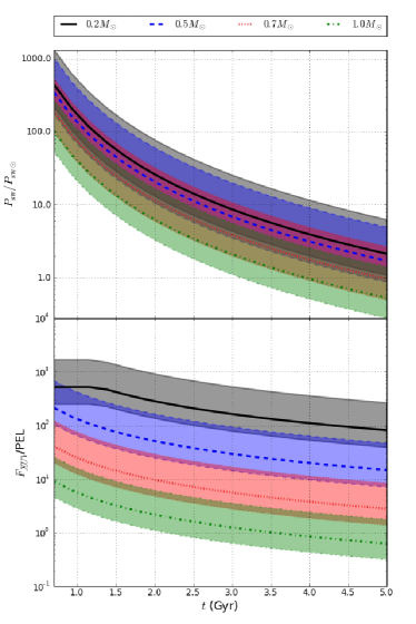
Figure 4.— Evolution of the stellar wind dynamical pressure (upper panel) and the XUV flux (lower panel) inside the HZ of a selected set of stellar masses.

2.3.3 Stellar XUV fluxes

The XUV luminosity of a star depends on its level of chromospheric and coronal activity which in turn depend on the rotation rate of the star. It is now well known that the rotation of main sequence stars slows down with age. It follows from there that the XUV luminosity should also decrease monotonically in time. Estimating the variation in time of the XUV luminosity for stars of different spectral types is harder than thought. There is a large dispersion of rotation periods and hence in the XUV luminosity of stars of the same spectral type (Pizzolato et al. 2003). Differences in one order of magnitude have been observed in stars with the same age (see e.g. Micela et al. 1996). Additionally EUV radiation is absorbed by the interstellar medium and therefore we depend on proxies to estimate the total XUV luminosity, X-ray luminosity being the most common.

Using observational data and independent estimations of stellar ages several authors have developed empirical laws providing the value as a function of time of different XUV luminosity proxies, e.g. $L_{X}$ (see e.g. Ribas et al. 2005, Penz & Micela 2008, Penz et al. 2008, Lammer et al. 2009, Garcés et al. 2011). Given the implicit uncertainties in the estimation of $L_{\rm XUV}$ and to be consistent with our goal of obtaining the best case for magnetic protection, we have selected the model predicting the lowest values of the XUV luminosities. The empirical law obtained by Garcés et al. 2011 is the best suited for that purpose. According to that result the X-ray luminosity of GKM stars change over time following the simple power-law function:

$$L_{X}=\left\{\begin{array}[]{ll}6.3\times 10^{-4}L_{\star}&\rm{if}\;t<t_{i}\\ 1.89\times 10^{28}\;t^{-1.55}&\rm{otherwise}\end{array}\right.$$ (23)

where $L_{\star}$ is the bolometric luminosity of the star and $t_{i}$ is the end of the saturation phase that scales with $L_{\star}$ as,

$$t_{i}=0.06\,\rm{Gyr}\;\left(\frac{L_{\star}}{L_{\odot}}\right)^{-0.65}$$ (24)

Luminosities are in units of erg s^-1. For simplicity we assume $L_{\rm XUV}\approx L_{\rm X}$. Using this model the Present Earth Value of the XUV flux (thereafter PEL) is 0.64 erg cm^-2 s^-1 which, as expected, underestimates the observed value of this quantity (Judge et al. 2003; Guinan et al. 2009).

In figure 4 we plot the value of the XUV flux as a function of time as measured in the HZ of four different stars. XUV fluxes in the range of $10-1000$ PEL seem to be common in early phases of stellar evolution posing severe constraints on the survival of planetary atmospheres of unmagnetized and weakly magnetized planets. We will return to this point in section 4.

3. Atmospheric thermal expansion and mass-loss

One of the most critical points regarding the survival of the atmospheres of low-mass planets is the fact that in the early phases of stellar evolution they would be under extreme conditions of X and EUV irradiation. A highly irradiated and relatively light atmosphere will have high levels of thermal and non-thermal mass-losses especially if it is unprotected against the action of the stellar wind. It has been estimated that under no or even a weak protection from an intrinsic magnetic field a TP could lose its atmosphere or most of its volatile content in a time-scale much shorter than that required for the evolution of life (see e.g. (Lammer et al. 2012)). Understanding the relation between the XUV-induced atmospheric expansion and mass-loss, and the properties of the planetary magnetosphere is of fundamental importance in assessing the problem of magnetic protection.

The key property in distinguishing between a magnetically protected atmosphere and an exposed one is the radius of the exobase $R_{\rm exo}$, defined as the distance where the mean-free path of atmospheric particles could be comparable to the size of the planet. This is the limit where atmospheric particles, given the proper energetic or flux conditions, could escape from the planetary atmosphere. The height of the exobase depends on many complex factors ranging from the opacity of the atmopsheric gasses to the high energy radiation from the star, the interaction between the charged and neutral components of the high atmosphere and a complex network of chemical and photochemical reactions of the atmospheric constituents (for a complete description see Tian et al. 2008). All these factors are critically determined by the chemical composition of the atmosphere. In the last few years several authors have, using detailed chemical, thermal and hydrodynamical models of TPs atmospheres, calculated the exosphere properties for two chemical compositions: N₂ rich or Earth-like composition atmospheres (Watson et al. 1981; Kulikov et al. 2006; Tian et al. 2008) and dry CO₂ or Venus-like composition atmospheres (Tian 2009; Lammer et al. 2012).

In order to include this important component in our comprehensive model we have used here the exospheric properties computed with two different models: a N₂ rich atmosphere of an Earth-like planet (Tian et al. 2008) and a CO₂ rich atmosphere of massive SEs $M_{p}>6M_{\oplus}$ (Tian 2009). The radius of the exobase in these models as a function of the XUV flux is depicted in figure 5. We see that N₂ rich atmospheres of Earth-like planets expand further than $\sim 10R_{p}$ at XUV fluxes larger than $\sim 20$ PEL. In this case the atmosphere become exposed even if they have the maximum level of magnetic protection, i.e. $R_{S}\sim 10R_{p}$ and could be stripped off by thermal and (stellar-wind related) non-thermal mass-losses. On the other hand, CO₂ rich atmospheres are cooled off efficiently through the emission of IR-radiation in the 15 $\mu$m CO₂ band and become able to withstand higher XUV levels.

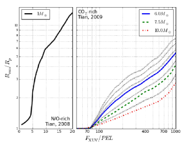
Figure 5.— Radius of the exobase for the models used in this work. Left panel corresponds to an Earth-mass planet with a N/O-rich atmosphere. Right panel shows the exobase radius for super-Earths with CO₂-rich atmospheres. Dotted lines in the right panel are the linearly interpolated and extrapolated exobase radius for masses from top to bottom 3.5, 4.5, 5.5, 7.0 and 9.0 $M_{\oplus}$. XUV fluxes are expressed in terms of the present Earth level, $PEL\approx 5$ mW/m².

In order to evaluate if a TP is magnetically protected we will compare the evolving value of the exobase radius and the standoff distance computed with our dynamical magnetosphere model. It is expected that at the earliest phases of stellar and planetary evolution the exobase radius would be larger than the standoff distance irrespective of the existence of an intense early dynamo. To expect that the magnetosphere protects the planetary atmosphere from the very beginning is simply unrealistic. Therefore the critical property to evaluate the level of magnetic protection of a given planet is the time $\Delta t_{\rm exp}$ during which this exposition state is maintained. More precisely the total atmospheric mass lost during this interval $M_{\rm exp}$ will give us the information we require to determine if the planetary atmosphere can survive the early “aggression” of its host star. We return to these important properties of the magnetic protection evolution in the next section.

4. Results

Combining all the elements of our comprenhensive model we have calculated the evolving magnetic protection conditions of potentially habitable TPs.

We have caclculated and compared the level of magnetic protection for planets in the mass range $0.7-10\,M_{\oplus}$ in three different cases: 1) instantaneous values of the magnetosphere and exosphere properties, especially at the earliest phases of the thermal evolution ($t\approx 1$ Gyr), 2) evolution in time of the same properties during a time-scale comparable to the development of complex life ($t=1-3$ Gyr) and 3) the cummulative atmospheric mass-loss of major constituents in the same period of case 2.

We study these three cases for three type of planets: a) hypothetical planets in the mass-range $0.7-10\,M_{\oplus}$, b) an Earth-twin, i.e. a habitable planet with the same mass and period of rotation than the Earth, but orbiting different type of stars and c) the Earth-like planets and SEs already discovered inside the HZ of their respective host stars, including, for reference purposes, Venus and the Earth itself. In table 2 we summarize the properties of the planets in the last group.

Planet	$M_{p}(M_{\oplus})$	$R_{p}(R_{\oplus})$	a(AU)	$P_{o}$ (days)	e	S-type	$M_{\star}(M_{\odot})$	$R_{\star}(R_{\odot})$	age(Gyr)	tid.locked
Earth	1.0	1.0	1.0	365.25	0.016	G2V	1.0	1.0	4.56	No
Venus	0.814	0.949	0.723	224.7	0.007	G2V	1.0	1.0	4.56	Probably
GJ 667Cc	4.545	1.5*	0.123	28.155	$<0.27$	M1.25V	0.37	0.42	$>2.0$	Yes
HD 85512b	3.496	1.4*	0.26	58.43	0.11	K5V	0.69	0.53	$5.6-8.0$	Yes
Gl 581d	6.038	1.6*	0.22	66.64	0.25	M3V	0.31	0.29	$4.3-8.0$	Yes

Table 2Properties of already discovered SEs inside the HZ of their host stars. For reference purposes the properties of Venus and the Earth are also included. Values of radii marked with an $*$ are unknown and were estimated using the mass-radius relation for planets with the same composition as the Earth, i.e. $R_{p}=R_{\oplus}(M_{p}/M_{\oplus})^{0.27}$ (Valencia et al. 2006).

To include the effect of rotation in the properties of the PMF we have assumed that planets in the HZ of late K and dM stars ($M<0.6M_{\odot}$) are tidally locked and therefore their periods of rotation are equal to their orbital periods (n=2 in eq. 16). For planets that preserve their primordial periods of rotation we assume values for $P$ in the range $1-100$ days as predicted by models of planetary formation (Miguel & Brunini 2010) with $P=1$ day as the preferred reference value.

Figures 6 and 7 show the evolution of magnetosphere properties for tidally locked and unlocked habitable planets. In all cases we have assumed that the planets are in the middel of the HZ. Even in early times tidally locked planets of arbitrary masses have a non-negligible magnetosphere ($R_{S}>1.5\ R_{p}$). As the star evolves the dynamical pressure of the stellar wind decreases more rapidly than the dipole moment (see figures 2 and 4) and the standoff distance grows. The critical boundary observed in the middle and rightmost panels are a product of the inner core nucleation. Planets to the right of the boundary created by a concentration of isolines still have a liquid core and therefore develop lower dipole moments. On the other hand, the inner core in planets to the left of the same boundary have already started to grow before that time and therefore their dipole moments are much larger.

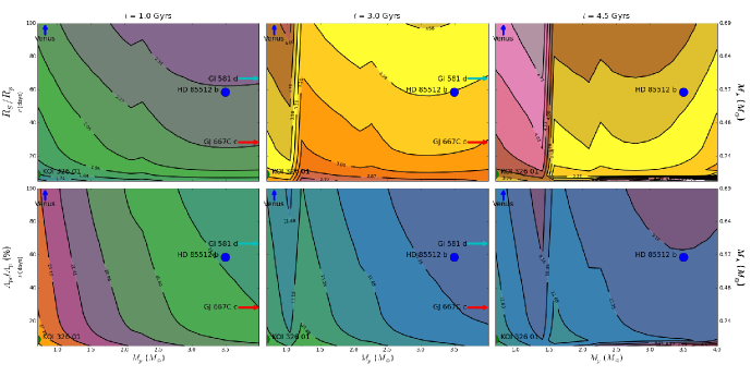
Figure 6.— Evolution of the standoff radius and polar cap area for tidally locked planets: the period of rotation of each planet is assumed equal to the orbital period at the middle of the HZ of low mass stars $M_{\star}<0.6M_{\odot}$ (ticks on the right vertical axis). The position of already discovered potentially habitable TPs is indicated with a circle or with an arrow when their properties fall beyond the axis limits.

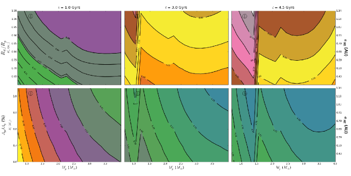
Figure 7.— Same as figure 6 but for unlocked planets with constant period of rotation $P=1$ day.

Previous estimates of the standoff radii for tidally locked planets are lower than the values reported here. For example, Khodachenko et al. 2007 place the range of standoff distances well below $2\ R_{p}$ even under mild stellar wind conditions (see figure 4 in their work). This is easily explained since they also underestimate the maximum dipole moment for this type of planet. While they predict maximum dipole moments for tidally locked planets around stars with $M_{\star}\approx 0.5M_{\odot}$ in the range of 0.022 to 0.15 ${\cal M}_{\oplus}$, our model predicts dipole moments as large as 0.8 ${\cal M}_{\oplus}$ for planets with the largest mass and at times as early as $t\approx 1$ Gyr.

A lower standoff distance means a larger polar cap. Tidally locked planets, even under the assumption that their exobases are not larger than the magnetosphere, have more than 15% of their atmospheric surface area exposed to open field lines where thermal and non-thermal processes could efficiently remove atmospheric gasses. Moreover, our model predicts that this type of planet will probably have multipolar PMF (thereafter paleomagnetospheres) which only increase the areas where field lines are open to the interplanetary space and magnetotail regions (Stadelmann et al. 2010).

Unlocked planets (figure 7) as expected seem to be best protected by extended magnetospheres $R_{S}>4\ R_{p}$ and lower polar cap areas $A_{\rm pc}<10\%$. It is interesting to notice that in both cases and at early times $t\approx 1$ Gyr a smaller planetary mass also implies a lower level of protection. This fact seems to contradict the idea that low-mass planets ($M_{p}<2.5$) are best suited to develop intense PMF (Gaidos et al. 2010; Tachinami et al. 2011; Zuluaga & Cuartas 2012). This apparent contradiction is explained by taking into account that the early dynamo generated magnetic fields of planets with very different masses are of the same order (see e.g. figure 8 in Gaidos et al. 2010): although larger planets produce more convective energy, the oversized liquid core and a larger planetary radius produce a surface magnetic field similar in intensity to that of a smaller planet. Having similar surface PMF, planets with larger masses will have much larger dipole moments, ${\cal M}\sim R_{p}^{3}$ and under the same stellar conditions will be best protected against the action of the stellar wind. This situation is not longer valid when low-mass SEs ($M_{p}<2.5$) develop an inner core and the available energy for convection is largely increased.

We have also calculated the standoff distance and polar cap area for different evolutionary stages of the already discovered habitable planets enumerated in table 2. The position are indicated with circles, whose size is proportional to their measured or estimated planetary radii, in the contour plots of figures 6 and 7. Planets whose properties are out of the ranges used in these figures are indicated with arrows at the border of each panel.

A more detailed account of the evolution of magnetosphere properties for already discovered habitable planets is presented in figure 8. The values of magnetosphere properties at the present age of the planet are indicated with circles whose size is proportional to the planetary radii. The case of Venus and that of the Earth are also included for reference purposes.

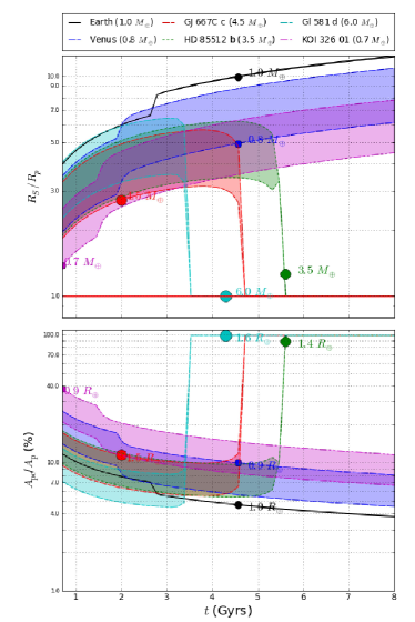
Figure 8.— Evolution of magnetosphere properties for already discovered habitable SEs. Shaded regions are limited by the properties determined with the minimum ($P\approx 1$ day) and maximum period of rotation of the planet ($P\approx P_{o}$).

In all cases we have used values for the period of rotation ranging from a minimum, corresponding to an assumed primordial rotation rate of $P_{\rm min}=24$ h (with exception of the Earth for which we have used $P_{\rm min}=17$ h), and a maximum, equal to the orbital period (tidally locking). The minimum and maximum values of the rotation period determine the upper (lower) and lower (upper) boundaries of the shaded regions in the upper panel (lower panel) respectively.

The case of Venus is particularly interesting in order to analyse the rest of the planets. The dynamo of Venus probably shut down at $t=3$ Gyr as a consequence of the drying of the mantle (Christensen et al. 2009). A massive loss of water induced by a runaway greenhouse and unsufficient early magnetic protection played a central role in the extinction of the early Venusian PMF. The case of Gl 581 d, GJ 667Cc and HD 85512b, though similar to Venus, is much more complex. On one hand their masses are larger than Venus’ and therefore their gravity could provide additional protection to the atmospheric mass-loss. On the other hand, their dynamos shut down in times $t\approx 3-5$ Gyr exposing them to the direct action of the stellar wind. In G and K stars this situation could not be consider a big threat since the stellar wind had also decreased its intensity when the planet lost its PMF (see figure 4), this will also be the case for HD 85512b. However, Gl 581d and GJ 667Cc are located at the HZ of dM stars where the stellar wind pressures, even at times as late as 4 Gyr, are intense enough to massively erode their atmospheres or to make them lost their volatile content.

As explained in section 3 the magnetic protection of a habitable planet is not only a function of the magnetopshere properties. In order to asses the problem we need also to evaluate the effect of the XUV radiation in the outer atmosphere expansion. In figure 5 we compare the evolution of the exobase radius and the standoff distance for two representative TPs planets: an Earth-mass planet with a N/O-rich atmosphere in the HZ of G-K stars and a super-Earth with $M_{p}=6M_{\oplus}$ and a CO₂-rich atmosphere in the HZ of dM stars $M_{\star}<0.6$. For the Earth-mass planet we have assumed periods of rotation in the range $P=1-10$ days which are compatible with TP formation theories (Miguel & Brunini 2010). For the rotation rate of the super-Earth we have assumed rotation periods of between 1 day (primordial rotation) and the orbital period (tidally locked case). Both planets were placed at the middle of the HZ of each star. Standoff distances for the HZ of stars in the mass-range studied in each case do not change significatively. For reference purposes we have only plotted this quantity for the star with the largest mass in the interval considered in each case (1.0 $M_{\odot}$ for the upper panel and 0.5 $M_{\odot}$ for the lower panel)

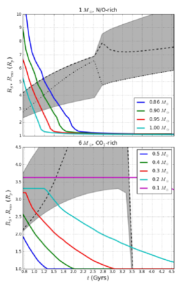
Figure 9.— Radius of the exobase (solid lines) and standoff distance (shaded area) as a function of time for two potentially habitable TPs. Upper panel: Earth-mass planet with a N/O-rich atmosphere. The shaded region corresponds to the standoff distance computed for a solar-mass star and assuming periods of rotation of 1 day (upper limit) and 10 days (lower limit). Dashed line is for $P=1.5$ days and dash-dotted line is for $P=3$ days. Lower panel: massive super-Earth with a CO₂-rich atmosphere. The shaded region corresponds to the standoff distances calculated in the HZ of a star with $0.5M_{\odot}$ and periods between 1 day (upper limit) and the orbital period (tidally locked case, lower limit). Dashed line corresponds to a rotation period $P=4$ days or approximately 1/17th of the orbital period.

For a solar-mass star and $P=1$ day (dipolar dominant early PMF), the exposure time is $\Delta t_{\rm exp}\approx 200$ Myr. However, if the primordial period of rotation is 3-5 days (multipolar field) the exposure could be increased by up to 1 Gyr threatening the atmospheric stability or its content of volatiles. The exposure time for an Earth-mass planet increases monotonically when it is located at closer distances to late G and early K stars. If the Earth-mass planet is located in the middle of the HZ of a star with $M_{\star}<0.86$ ($a_{\rm HZ}\approx 0.80$ AU) it would be subject to levels of XUV irradiation high enough to blowing off the atmosphere. This fact points to the existence of a subregion of the HZ that we can call a Magnetic-restricted Habitable Zone (MHZ), where planets with a given mass and atmospheric composition could preserve their atmospheres. It is interesting to note that although Venus was inside the solar HZ during the first Gyr of the solar system evolution it has always been outside of the MHZ for Earth-like planets with N/O-rich atmospheres. CO₂ rich atmospheres which are less propense to expand, i.e. $R_{\rm exo}<2$ for $F_{\rm XUV}\sim 100$ (Kulikov et al. 2006) are probably protected at the critical early phases of planetary evolution, provided the planet preserves the conditions required for dynamo action (e.g. an hydrated mantle, mobile lids, etc.) In that case the MHZ will extend to stars with lower masses or closer habitable distances.

The case for massive super-Earths in the HZ of dM stars has several interesting differences with respect to the magnetic protection of Earth-mass planets. The continued activity of very late dM stars ($M_{\star}\sim 0.1$) will produce a constant level of XUV irradiation and hence a constant exobase radius during times longer that the dynamo life-time itself (magenta solid line). Under this condition and assuming that the planet is tidally locked in the first Gyr, the atmosphere will be permanently exposed and will probably be subject to large thermal and non-thermal mass-losses. However, for stars with masses $M_{\star}\gtrsim 0.2$ a tidally locked planet will only be exposed during few Myr to 1.0 Gyr. If the mass-loss is not too large (Tian 2009) the planetary atmosphere could survive the initial stellar aggression. Again we could identify here a minimum stellar mass (HZ distance) for which the atmosphere is critically exposed. For a tidally locked 6 $M_{\oplus}$ super-Earth that minimum mass is close to 0.3 $M_{\odot}$ ($a_{\rm HZ}\approx 0.15$ AU). The inner limit of the so-called MHZ is farther away for SEs with larger masses but still covers a significant fraction of the tidally locked region of the HZ.

In order to quantify in more detail the effect that the early exposition to the stellar wind has on the atmosphere erosion of habitable TPs we have calculated the exposure time and the total mass loss during this critical period for an Earth-mass planet in the HZ of G-K stars and tidally locked SEs. The results are presented in figure 10.

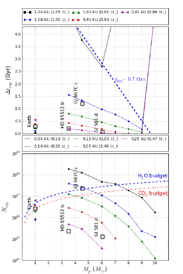
Figure 10.— Exposure time $\Delta t_{\rm exp}$ and mass-loss $M_{\rm exp}$ as a function of planetary mass for two atmospheric compositions: N/O-rich atmospheres (Earth-mass planet) and CO₂-rich atmospheres (super-Earths). Planets were placed at different distances from their host stars (see legends). For each distance the mass of the star, where that distance corresponds to the middle of the HZ, is indicated in parenthesis. For the Earth-mass planet we assumed a constant period of rotation $P=1$ day. The super-Earths were placed in the HZ of dM stars and are tidally locked, i.e. $P=P_{o}$. For reference we have included the duration of the dynamo $t_{\rm dyn}$ with respect to the initial time (0.7 Gyr) (upper panel, dashed line) and the CO₂ and H₂O content scaled with the Earth’s mass (dahed and dash-dotted lines in the lower panel). The exposure time and mass-loss predicted for the already discovered habitable planets are marked with squares.

In the case of super-Earths we have used the flux of carbon reported in figure 8 of Tian 2009. For masses not included in the simulations we have linearly interpolated and extrapolated the already reported results for planets with masses of 6, 7.5 and 10 $M_{\oplus}$. The flux of oxygen, the most abundant ion in higly irradiatend N/O-rich atmospheres, in the case of the Earth-mass planet, was calculated multiplying the estimated number density $n$ as estimated from the exobase definition (eq. 18 in Kulikov et al. 2006) and the exobase bulk velocity reported in figure 8d of Tian et al. 2008. In both cases the total mass-loss is compared with the assumed initial content of CO₂ ($2.5\times 10^{46}$ for an Earth-mass planet, Tian 2009) and the amount of water in the planetary hydrosphere ($4.6\times 10^{46}$ molecules for an Earth-mass planet, Kulikov et al. 2006). For planets with a mass larger than that of the Earth and for the sake of simplicity these initial content of critical volatiles were scaled linearly with mass.

We have observed that exposure time and mass-loss, depend on the distance from the star but are almost independent of the stellar mass compatible with that distance. Therefore, an Earth-mass planet placed at $\sim 0.8$ AU will be subject to a comparable exposure around a 0.75 $M_{\odot}$ where that distance correspond to the outer boundary of the HZ (see figure 3) or around a 0.86 $M_{\odot}$ star (middle of the HZ) or around a 1.05 $M_{\odot}$ star (inner boundary of the HZ). This is the reason why we have decided to parametrize the results in terms of the planetary distance from the star rather than in terms of stellar mass as in figure 9.

The exposure times for the Earth-mass planet are compatible with the results presented in figure 9. The early mass-loss for this type of planet ranges from 25% of the scaled mass of the ocean for a distance 20% larger than present Earth, to a value larger than this critical threshold for a planet 20% closer than the Earth. The exposure time and mass-loss for tidally locked super-Earths decrease with mass as expected from the decreasing of the exobase radius with an increasing planetary mass (see figure 5. We confirm here the existence of a minimum distance for a given planetary mass beyond which the carbon mass-loss is below the expected CO₂ content. For example, a super-Earth with mass $6M_{\oplus}$ located at distances larger than 0.1 AU (long dashed lines in the lower panel) will always have mass-losses below that threshold. This limit corresponds to the middle of the HZ around a $0.2M_{\odot}$ star which confirms the analysis derived from figure 5.

With the information at hand and assuming that the already potentially habitable super-Earths have similar compositions to the Earth and CO₂ rich atmospheres we can conclude that GJ 667Cc has already lost a significant fraction of its atmospheric mass and it is probably now uninhabitable. Gl 581d and HD 85512b seem to be in a safe region of the parameter space. Altough our model provides a very conservative estimate of the early exposure conditions, the estimated mass-losses for both planets are more than one order of magnitude below the critical threshold. Even if we accept that their dynamos are weaker or if we include the additional mass-loss produced after their dynamos shut down (see figure 8) the total mass-losses are still below the scaled CO₂ content.

5. Discussion and further analysis

This is the first attempt to integrate into a single comprehensive model all the relevant physical phenomena involved in the magnetic protection of habitable planets. Although several components of the model are expecting important improvements in the following years (bulk properties of low-mass stars and their evolution, structure and evolution of stellar winds, physics of highly irradiated atmospheres, atmospheric escape in magnetized planets) the esential elements have been put together to produce an integrated view of the role of magnetic fields in the survival of the atmosphere of habitable TPs.

One important source of uncertainties in our model, especially when applied to already discovered TPs, is the assumption that all of them have similar compositions to the Earth. Planets with elemental and mineralogical compositions different to our planet are probably more abundant than previously thought (Bond et al. 2010). Although numerical models of the bulk interior of solid planets with very different compositions have already been computed (Seager et al. 2007) the detailed structure, mineralogical phases, thermal profiles and evolution, among other geophysical relevant information, are waiting to be studied in more detail for this type of planet. Plate tectonics, mantle rheology, additional interior heating sources (e.g. radioactive and tidaly heating) and the formation, composition and thermal structure of a metallic core are key properties to study the thermal and magnetic field evolution on planets with very different composition to the Earth.

Gaidos et al. (2010) have studied the effect that an increased core size (larger Fe/Si ratio) or a different amount of radionuclides have on the thermal evolution and hence the PMF evolution of planets with different composition than the Earth. They found that increasing the Fe/Si ratio for an Earth-mass planet, i.e. increasing the radius of the core, will have two effects on the thermal and magnetic field evolution (see figure 7 in their paper): 1) an earlier formation of the solid iron core and 2) more intense surface fields (mainly due to a reduction in the distance between the planetary and core surface without a significant change in the convective power). A change in the predicted magnetic field intensity of almost one order of magnitude was observed changing the core radius between 0.5 and 1.5 times the Earth’s core radius. Using equations 1 and 5 it is predicted that a larger relative amount of Fe could imply a standoff distance of up to 3 times larger than that predicted for a planet with a composition similar to Earth. Also an earlier inner core formation would imply increased magnetic protection during the critical earlier phases of stellar and planetary evolution. The effect of a different amount of radionuclides on the PMF strength is negligible (see figure 7 in Gaidos et al. 2010). In all these cases the magnetic protection conditions predicted here will be improved. Thus, for example, GJ 667Cc will have better chances of preserving its atmosphere if its content of Fe is much larger than that of the Earth.

The effect of different rheological properties and thermal structure on SEs have also been studied in the detailed mantle and core thermal evolution by Tachinami et al. (2011). Although they also assumed the same elemental and mineralogical composition as the Earth the attention they put on the role of variations in the rheological properties of the mantle and different thermal conditions at the core mantle boundary (CMB) could be helpful in roughly guessing what could happen on planets with different compositions. They have found that the total lifetime and surface strength of the PMF are sensitive to changes in these properties (see figure 11 in Tachinami et al. 2011). Changes become particularly important for planets with masses larger than the Earth ($M_{p}>2M_{\oplus}$). For example, they predict that the metallic core of planets with a mass as large as 5 $M_{\oplus}$ could actually cool enough to develop an inner solid core, provided that on one hand the viscosity of the mantle is weaker dependent on pressure and on the other hand, that the temperature contrast through the CMB is up to 10 times larger than that expected for the Earth. In this case larger-mass-planets could develop strong PMF and its magnetic protection could be ensured even at closer distances to their host star than those predicted here.

We have simulated the previously discussed effects by changing the fitting parameters of the phenomenological functions describing the thermal evolution (equations 7-9 and scaling parameters in table 1). We present in figure 11 the results of this “test of sensitivity” to our model of variations in the thermal evolution details. We have plotted the percentual variation of the standoff distance and the factor of variation in the total mass-loss when the following properties of the thermal evolution are modified with respect the nominal values used in this work: 1) the radius of the metallic core $R_{c}$ (scaling parameter $\alpha_{\rm Rc}$), 2) The time of inner core nucleation $t_{i}c$ (scaling parameter $\alpha_{\rm tic}$) and 3) the critical mass for solid inner core nucleation, $M_{\rm crit}$.

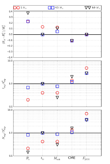
Figure 11.— Test of the model’s sensitivity to changes in the parameters of the thermal evolution model ($R_{c}$, $t_{\rm ic}$ and $M_{\rm crit}$) and the stellar wind and XUV irradiation properties (coronal mass ejection conditions or CME and $F_{\rm XUV}$). The value of the magnetic protection key quantities $R_{S}$, $t_{\rm exp}$ and $N_{\rm exp}$ are compared with their nominal values $R_{S}^{0}$, $t_{\rm exp}^{0}$ and $N_{\rm exp}^{0}$ as calculated with the set of physical parameters used in this work.

We see that the value of standoff distance predicted by the model is very robust. Most of the modification of the model parameters produce changes in the nominal value of only $\sim$ 20% or less. This could be explained by the weak dependence of the standoff distance on the dipolar moment, eq. (5) $R_{S}\sim{\cal M}^{1/3}$. Only when the core radius is increased (we have used $R_{C}\approx 1.2R_{C}^{0}$ where $R_{C}^{0}$ is the nominal core radius scaled with the mass of the Earth) is a difference in the standoff radius of 40% observed in the case of massive SEs. For planets with lower masses the difference is still around the 20% limit.

The exposure time and mass-loss are much more sensitive to changes in the thermal evolution parameters. This is explained taking into account that even small variations in the standoff distance could increase by a factor of 2-5 the time during which the planet is exposed directly to the stellar wind erosion. As expected the largest changes are observed when we change the core radius (Fe/Si ratio). The predicted mass-losses for EPs and massive SEs are almost 10 times lower than those obtained with the nominal model. SEs with intermediate mass ($M_{p}\sim 4M_{\oplus}$) are less sensitive to core radius changes and the mass losses decrease by a factor of 2 only, when the core radius is increased. These results support to the conclusion that Gl 581d and HD 85512b would be well protected by their planetary dynamos (if they actually exist or existed in the past) but that GJ 667Cc has been too exposed to the erosive action of the stellar wind and probably has lost its atmosphere or its content of critical volatiles.

In our conservative model we neglected the effect that an enhanced early stellar magnetic activity would have in the early erosion of the magnetically protected atmospheres, especially in the case of close-in planets around dM stars. It is interesting to consider how our results could be affected if a planet were exposed to more stressful conditions, e.g. coronal mass ejections and/or higher levels of XUV irradiation. We have performed sensitivity tests to study the effects of an enhanced stellar wind and larger fluxes of XUV radiation such as that expected for very active stars. To achieve this we modify the stellar wind pressure by maintaining the nominal velocity of the plasma (as predicted by the Parker’s model) but increasing by a factor of 2 the density of stellar wind plasma. For the XUV flux we multiply by 2 the nominal XUV luminosity of G-K stars (Earth-mass planet) and maintain the initial high value of the XUV luminosity of dM stars (4.5 and 6.0 $M_{\oplus}$ cases) simulating an extended period of stellar activity. The results of these sensitivity tests are depicted in the CME and $F_{\rm XUV}$ columns in figure 11.

CME conditions change the standoff radius is only 10%. Again this could be explained by the weak dependence of this quantity on the stellar wind pressure and in particular to the number density of wind particles, eq. (5) $R_{S}\sim P_{\rm sw}^{-1/6}\sim n^{-1/6}$. A sustained increase in the XUV fluxes does not modify the standoff distance at all but it is able to noticeably increase the exobase radius and hence the time of exposure to the stellar wind erosion. As expected, the planet more susceptible to this effect is the Earth-mass planet which has a N/O-rich atmosphere. Even under harsh conditions of stellar aggression the mass-losses for TPs, irrespective of their mass, are no larger than 10 times the nominal value. Again this reinforces the conclusion that Gl 581d and HD 85512b are well protected by their potential PMFs.

The existence of mobile lids is also a key factor for the existence of strong enough PMFs on habitable planets and it is required for the validity of the thermal evolution model results used in this work. The problem is being explored from different perspectives and using complimentary methodologies (see e.g. Valencia et al. 2007 and O’Neill & Lenardic 2007. A consensus about the possibility of planets with greater mass having or not having lid activity has not yet been reached. However, different lines of evidence point to the fact that, in a wide range of rheological and thermal paramters, mobile lids could be common in planets up to $10M_{\oplus}$ (for recent results see e.g. Noack et al. 2012).

To estimate the radius of the exobase our model relies on the results of detailed hydrodynamical and thermodinamic models of highly irradiated atmospheres of TPs. However, we have used results calculated for two different types of atmosphere. Although in nature atmospheric composition could also depend on planetary mass, for reliable comparisons it is better to use a single model. We also have a “void” in model results for planets in the mass range $1-6M_{\oplus}$. Although we have filled the $3.5-6$ $M_{\oplus}$ mass range using a simple linear extrapolation it is expected that future improvements to the atmospheric models will provide reliable values for the exosphere properties for planets in that interval of masses. We are confident however that the exobase radius will not be too different from that used in this work and the main qualitative conclusions will not be modified significantly.

6. Summary and Conclusions

In the last few years we have seen significant improvements in the understanding of the role that planetary magnetic fields could have in the stability of the atmopsheres of exoplanets. In line with these advances in this paper we have developed a comprehensive model of the evolution of magnetic protection of potentially habitable TPs, integrating in a single framework the results from very different specific areas of research in this field: thermal evolution of solid planets, scaling of dynamo-generated magnetic fields, magnetosphere modeling, physical properties of low-mass stars, stellar wind evolution and atmospheric modeling of highly irradiated planets.

Using this model we have studied the magnetic protection of hypothetical habitable TPs in a wide range of planetary masses and have addressed for the first time the cases of the already discovered TPs found in the HZ of their host stars. In all these cases we have estimated the evolution of two key properties: the magnetopshere size as measured by the standoff distance and the radius of the exobase. The direct comparison between these properties gives us information about the evolution of the protection that the magnetosphere provides to the planetary atmosphere against the erosive action of the stellar wind. In order to estimate at to extent this magnetic protection prevents the loss of a significant fraction of the mass of the atmosphere or the loss of large amounts of critical volatiles (e.g. H₂O and CO₂) we have estimated the thermal-induced mass-loss. Knowing that non-thermal losses could be much larger, our conservative model provides an underestimation of the stellar wind exposure effect. The potentially habitable TPs that under our model result in unsuitable conditions for magnetic protection in reality are even worse than the model predicted.

Our model is sensitive to a number of factors that affect the quantitative results we have obtained here. We have studied the sensitivity of our results to the expected variations in the model parameters and observed that the global conclusions are still very robust.

We confirm that Earth-like planets, irrespective the composition of their atmospheres and even under the highest attainable dynamo-generated magnetic field strengths, will lose a significant fraction of their atmospheres or their critical volatile content if they are tidally locked in the HZ of dM stars. The case for the absence of habitable Earth-like planets around this type of star are almost closed. The case of habitable EPs around GK stars is not as good as previously expected either. Earth-mass planets with N/O-rich atmospheres, even under the best conditions of magnetic protection, will probably lose their atmospheres or their content of water if they are in HZ closer than $\sim$ 0.8 AU. This limit excludes a large range of stellar masses (0.6-0.9 $M_{\odot}$) depending on the particular region inside the HZ (close to the inner or outer limit) where the planet resides.

super-Earths with $M_{p}\gtrsim 3M_{\oplus}$ seem to have better chances of preserving their atmospheres even if they are tidally locked around dM stars. Under similar conditions of thermal and magnetic evolution there seems to exist a planetary mass-dependent inner limit inside the HZ itself below which large atmospheric mass-losses are expected. We coined here the name Magnetically-restricted Habitable Zone or MHZ for this hypothetical subregion and expect that it could be confirmed by future improvements in the model. This inner limit decreases with increasing planetary mass. Under the nominal value of the parameters used in our conservative model we predict that for $4M_{\oplus}$ planets the limit is close to 0.15 AU, while for $8M_{\oplus}$ it will be approximately 0.04 AU. It implies that planets with $M_{p}\leqslant 4M_{\oplus}$ in HZs closer than 0.15 AU will be too exposed and probably lose their habitable conditions in the first few Myr to 1 Gyr. This is precisely the case of Gj 667Cc that we predict here although inside the HZ of its host star it is currently uninhabitable given the early loss of its atmospheric content. Very massive SEs ($M_{p}>8M_{\oplus}$) will not have, under our conservative estimates, any restrictions and could preserve their atmospheres even if they are in the HZ of the lowest mass dM stars.

The already discovered potentially habitable SEs Gl 581d ($M_{p}=6.0M_{\oplus}$, $a=0.22$ AU) and HD 85512b ($M_{p}=3.5M_{\oplus}$, $a=0.26$ AU), if assumed similar in composition to Earth, are well inside the MHZ for their respective masses. Even if they are subjected to larger levels of stellar aggression their atmospheres seem to have been safe against the strong early erosion and probably still are there.

References

- Baraffe et al. (1998) Baraffe, I., Chabrier, G., Allard, F., & Hauschildt, P. H. 1998, A&A, 337, 403
- Batalha et al. (2012) Batalha, N. M., Rowe, J. F., Bryson, S. T., et al. 2012, ArXiv e-prints
- Bond et al. (2010) Bond, J. C., O’Brien, D. P., & Lauretta, D. S. 2010, ApJ, 715, 1050
- Borucki et al. (2011) Borucki, W. J., Koch, D. G., Basri, G., et al. 2011, ApJ, 728, 117
- Boss (2006) Boss, A. P. 2006, ApJ, 644, L79
- Catanzarite & Shao (2011) Catanzarite, J., & Shao, M. 2011, ApJ, 738, 151
- Chaufray et al. (2007) Chaufray, J. Y., Modolo, R., Leblanc, F., et al. 2007, Journal of Geophysical Research (Planets), 112, 9009
- Christensen et al. (2009) Christensen, U., Balogh, A., Breuer, D., & Glaßmeier, K. 2009, Planetary Magnetism, Space Sciences Series of ISSI (Springer)
- Christensen (2010) Christensen, U. R. 2010, Space Sci. Rev., 152, 565
- Denis et al. (2011) Denis, C., Rybicki, K. R., Schreider, A. A., Tomecka-Suchoń, S., & Varga, P. 2011, Astronomische Nachrichten, 332, 24
- Engle & Guinan (2011) Engle, S. G., & Guinan, E. F. 2011, ArXiv e-prints
- Gaidos et al. (2010) Gaidos, E., Conrad, C. P., Manga, M., & Hernlund, J. 2010, ApJ, 718, 596
- Gaidos, E. (2011) Gaidos, E. 2011, Personal communication
- Garcés et al. (2011) Garcés, A., Catalán, S., & Ribas, I. 2011, A&A, 531, A7
- Grenfell et al. (2007) Grenfell, J. L., Stracke, B., von Paris, P., et al. 2007, Planet. Space Sci., 55, 661
- Grießmeier et al. (2010) Grießmeier, J.-M., Khodachenko, M., Lammer, H., et al. 2010, in IAU Symposium, Vol. 264, IAU Symposium, ed. A. G. Kosovichev, A. H. Andrei, & J.-P. Roelot, 385–394
- Grießmeier et al. (2007) Grießmeier, J.-M., Preusse, S., Khodachenko, M., et al. 2007, Planet. Space Sci., 55, 618
- Grießmeier et al. (2009) Grießmeier, J.-M., Stadelmann, A., Grenfell, J. L., Lammer, H., & Motschmann, U. 2009, Icarus, 199, 526
- Grießmeier et al. (2005) Grießmeier, J.-M., Stadelmann, A., Motschmann, U., et al. 2005, Astrobiology, 5, 587
- Grießmeier et al. (2004) Grießmeier, J.-M., Stadelmann, A., Penz, T., et al. 2004, A&A, 425, 753
- Guinan et al. (2009) Guinan, E. F., Engle, S. G., & Dewarf, L. E. 2009, in American Institute of Physics Conference Series, Vol. 1135, American Institute of Physics Conference Series, ed. M. E. van Steenberg, G. Sonneborn, H. W. Moos, & W. P. Blair , 244–252
- Heller et al. (2011) Heller, R., Barnes, R., & Leconte, J. 2011, Origins of Life and Evolution of the Biosphere, 37
- Joshi et al. (1997) Joshi, M. M., Haberle, R. M., & Reynolds, R. T. 1997, Icarus, 129, 450
- Judge et al. (2003) Judge, P. G., Solomon, S. C., & Ayres, T. R. 2003, ApJ, 593, 534
- Kaltenegger (2010) Kaltenegger, L. 2010, ApJ, 712, L125
- Kaltenegger et al. (2011) Kaltenegger, L., Udry, S., & Pepe, F. 2011, ArXiv e-prints
- Kasting (2010) Kasting, J. 2010, How to Find a Habitable Planet, ed. Kasting, J. (Princeton University Press)
- Kasting et al. (1993) Kasting, J. F., Whitmire, D. P., & Reynolds, R. T. 1993, Icarus, 101, 108
- Khodachenko et al. (2007) Khodachenko, M. L., Ribas, I., Lammer, H., et al. 2007, Astrobiology, 7, 167
- Kipping et al. (2012) Kipping, D. M., Bakos, G. Á., Buchhave, L. A., Nesvorny, D., & Schmitt, A. 2012, ArXiv e-prints
- Kite et al. (2011) Kite, E. S., Gaidos, E., & Manga, M. 2011, ApJ, 743, 41
- Kulikov et al. (2006) Kulikov, Y. N., Lammer, H., Lichtenegger, H. I. M., et al. 2006, Planet. Space Sci., 54, 1425
- Lammer et al. (2012) Lammer, H., Lichtenegger, H. I. M., Khodachenko, M. L., Kulikov, Y. N., & Griessmeier, J. 2012, in Astronomical Society of the Pacific Conference Series, Vol. 450, Astronomical Society of the Pacific Conference Series, ed. J. P. Beaulieu, S. Dieters, & G. Tinetti, 139
- Lammer et al. (2004) Lammer, H., Ribas, I., Grießmeier, J.-M., et al. 2004, Hvar Observatory Bulletin, 28, 139
- Lammer et al. (2003) Lammer, H., Selsis, F., Ribas, I., et al. 2003, ApJ, 598, L121
- Lammer et al. (2007) Lammer, H., Lichtenegger, H. I. M., Kulikov, Y. N., et al. 2007, Astrobiology, 7, 185
- Lammer et al. (2009) Lammer, H., Bredehöft, J. H., Coustenis, A., et al. 2009, A&A Rev., 17, 181
- Lammer et al. (2010) Lammer, H., Selsis, F., Chassefière, E., et al. 2010, Astrobiology, 10, 45
- Mayor & Udry (2008) Mayor, M., & Udry, S. 2008, Physica Scripta Volume T, 130, 014010+08
- Mead (1964) Mead, G. D. 1964, J. Geophys. Res., 69, 1181
- Micela et al. (1996) Micela, G., Sciortino, S., Kashyap, V., Harnden, Jr., F. R., & Rosner, R. 1996, ApJS, 102, 75
- Miguel & Brunini (2010) Miguel, Y., & Brunini, A. 2010, MNRAS, 406, 1935
- Newkirk (1980) Newkirk, Jr., G. 1980, in The Ancient Sun: Fossil Record in the Earth, Moon and Meteorites, ed. R. O. Pepin, J. A. Eddy, & R. B. Merrill, 293–320
- Noack et al. (2012) Noack, L., Breuer, D., & Spohn, T. 2012, Icarus, 217, 484
- O’Neill & Lenardic (2007) O’Neill, C., & Lenardic, A. 2007, Geophys. Res. Lett., 34, L19204
- Parker (1958) Parker, E. N. 1958, ApJ, 128, 664
- Peale (1977) Peale, S. J. 1977, in IAU Colloq. 28: Planetary Satellites, ed. J. A. Burns, 87–111
- Penz & Micela (2008) Penz, T., & Micela, G. 2008, A&A, 479, 579
- Penz et al. (2008) Penz, T., Micela, G., & Lammer, H. 2008, A&A, 477, 309
- Pepe et al. (2011) Pepe, F., Lovis, C., Ségransan, D., et al. 2011, A&A, 534, A58
- Pizzolato et al. (2003) Pizzolato, N., Maggio, A., Micela, G., Sciortino, S., & Ventura, P. 2003, A&A, 397, 147
- Preusse et al. (2005) Preusse, S., Kopp, A., Büchner, J., & Motschmann, U. 2005, A&A, 434, 1191
- Rauer et al. (2011) Rauer, H., Gebauer, S., Paris, P. V., et al. 2011, A&A, 529, A8
- Ribas et al. (2005) Ribas, I., Guinan, E. F., Güdel, M., & Audard, M. 2005, ApJ, 622, 680
- Sano (1993) Sano, Y. 1993, J.Geomag.Geoelectr., 45, 65
- Sanz-Forcada et al. (2011) Sanz-Forcada, J., Micela, G., Ribas, I., et al. 2011, A&A, 532, A6
- Sanz-Forcada et al. (2010) Sanz-Forcada, J., Ribas, I., Micela, G., et al. 2010, A&A, 511, L8
- Scalo et al. (2007) Scalo, J., Kaltenegger, L., Segura, A. G., et al. 2007, Astrobiology, 7, 85
- Schwenn (1990) Schwenn, R. 1990, Large-Scale Structure of the Interplanetary Medium, ed. Schwenn, R. & Marsch, E., 99
- Seager et al. (2007) Seager, S., Kuchner, M., Hier-Majumder, C. A., & Militzer, B. 2007, ApJ, 669, 1279
- Segura et al. (2010) Segura, A., Walkowicz, L. M., Meadows, V., Kasting, J., & Hawley, S. 2010, Astrobiology, 10, 751
- Selsis et al. (2007) Selsis, F., Kasting, J. F., Levrard, B., et al. 2007, A&A, 476, 1373
- Siscoe & Christopher (1975) Siscoe, G., & Christopher, L. 1975, Geophys. Res. Lett., 2, 158
- Siscoe & Chen (1975) Siscoe, G. L., & Chen, C.-K. 1975, J. Geophys. Res., 80, 4675
- Stacey (1992) Stacey, F. D. 1992, Physics of the Earth., ed. Stacey, F. D.
- Stadelmann et al. (2010) Stadelmann, A., Vogt, J., Glassmeier, K.-H., Kallenrode, M.-B., & Voigt, G.-H. 2010, Earth, Planets, and Space, 62, 333
- Tachinami et al. (2011) Tachinami, C., Senshu, H., & Ida, S. 2011, ApJ, 726, 70
- Tian (2009) Tian, F. 2009, ApJ, 703, 905
- Tian et al. (2008) Tian, F., Kasting, J. F., Liu, H.-L., & Roble, R. G. 2008, Journal of Geophysical Research (Planets), 113, 5008
- Underwood et al. (2003) Underwood, D. R., Jones, B. W., & Sleep, P. N. 2003, International Journal of Astrobiology, 2, 289
- Valencia et al. (2006) Valencia, D., O’Connell, R. J., & Sasselov, D. 2006, Icarus, 181, 545
- Valencia et al. (2007) Valencia, D., O’Connell, R. J., & Sasselov, D. D. 2007, ApJ, 670, L45
- Varga et al. (1998) Varga, P., Denis, C., & Varga, T. 1998, Journal of Geodesy, 25, 61
- Voigt (1995) Voigt, G. 1995, Handbook of atmospheric electrodynamics, ed. H. Volland, Vol. 2 (CRC Press), 333–388
- Ward & Brownlee (2000) Ward, P., & Brownlee, D. 2000, Rare earth : why complex life is uncommon in the universe, ed. Ward, P. & Brownlee, D.
- Watson et al. (1981) Watson, A. J., Donahue, T. M., & Walker, J. C. G. 1981, Icarus, 48, 150
- Weber & Davis (1967) Weber, E. J., & Davis, Jr., L. 1967, ApJ, 148, 217
- Wood et al. (2002) Wood, B. E., Müller, H.-R., Zank, G. P., & Linsky, J. L. 2002, ApJ, 574, 412
- Zuluaga & Cuartas (2012) Zuluaga, J. I., & Cuartas, P. A. 2012, Icarus, 217, 88