Interfacial Phenomena and Natural Local Time

Abstract

This article addresses a modification of local time for stochastic processes, to be referred to as natural local time. It is prompted by theoretical developments arising in mathematical treatments of recent experiments and observations of phenomena in the geophysical and biological sciences pertaining to dispersion in the presence of an interface of discontinuity in dispersion coefficients. The results illustrate new ways in which to use the theory of stochastic processes to infer macro scale parameters and behavior from micro scale observations in particular heterogeneous environments.

Keywords. Advection-dispersion, discontinuous diffusion, skew Brownian motion, mathematical local time, natural local time

2010 Mathematics Subject Classification.

1 Introduction and Motivating Example

The purpose of this article is to present some new results that call attention to the presence and effects of particular types of heterogeneity observed to occur in diverse geophysical and ecological/biological spatial environments. A few examples of interest to the authors are provided to highlight the occurrence of interfacial discontinuities, but one may expect that readers will easily be able to conceive of many others. Apart from the motivating examples, theoretical results are provided to illustrate the interfacial effects in ways that may prove useful in analyzing and interpreting more complex data sets.

The most basic empirical considerations involve various temporal measurements, e.g., breakthrough times, residence or occupation times, recurrence times and, as will be explained, a fundamental notion of local time.

Mathematical local time is a quantity with a long history in the theory of stochastic processes. It concerns a mathematical measure of the amount of time a stochastic process spends locally about a point, which we will refer to as mathematical local time in distinction with a modification introduced here to be referred to as natural local time. Starting with the celebrated theorem of Trotter [46] establishing the continuity of mathematical local time for standard Brownian motion, the general problem of determining necessary and sufficient conditions for continuity of local time for stochastic processes is an old and well-studied problem at the foundations of probability theory; see [17] for recent progress and insight into the technical depth of the problem for a large class of Markov processes.

While the present paper has little to offer to the mathematical foundations of the subject, observations from field and laboratory experiments are provided together with some theoretical results that point to new directions in this area from the perspective of applications and modeling of certain dispersive phenomena. At the most fundamental level, the issue involves the units of measurement. In particular, the units of mathematical local time in the context of dispersion of particle concentrations are typically those of spatial length. This is not unnatural in the mathematical context owing to the locally linear relationship between spatial variance and time when the dispersion coefficient is sufficiently smooth. However, as will be seen, this breaks down in the presence of an interface of discontinuity in the diffusion coefficient.

Effort is made to make this article accessible to a diverse audience by including some basic mathematical definitions and background theory. A complete and systematic treatment of essentially all of the underlying mathematical concepts can be found in [41]. We conclude this introductory section with an empirical example that serves to motivate and illustrate the role of a key mathematical construct, namely that of skew Brownian motion. This is followed by a section with additional empirical illustrations from the ecological and biological sciences. The emphasis of the paper is on mathematical theory and modeling. The main results demonstrate (i) the effects of general point interface transmission probabilities on breakthrough times and (ii) on residence times; (iii) symmetry (via martingale) relationships between interfacial transmission probabilities, dispersion coefficients, and skewness parameters; (iv) a special role for continuity of flux (conservation of mass) verses continuity of derivatives at an interface; (v) a special role for (natural) local time continuity in the determination of the transmission parameter at the interface.

Example A (Dispersion in Porous Media). The topic addressed in this paper originally initiated as a result of questions resulting from recent laboratory experiments designed to empirically test and understand advection-dispersion in the presence of sharp interfaces. e.g., experiments by [23], [20], [7]. Such laboratory experiments have been rather sophisticated in the use of layers of sands and/or glass beads of different granularities and modern measurement technology (see Figure 1).

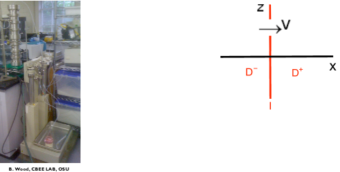
Figure 1: Saturated Fine/Coarse Grain Sand Separated by an Interface Experimental Assembly, Oregon State University

From an engineering science point of view, basic research in this area is aimed to improve understanding of the role of sharp discontinuities in the hydrologic parameters appearing in equations used for predictions of the spread of contaminants in saturated porous media. There is a huge literature in the sciences and engineering pertaining to the general problem. For a perspective on the mathematical foundations see [10], [8],[9], [48], [33], [6]. The former considers heterogeneity from a deterministic framework, while the latter involve randomness in the medium. [13] contains a survey of various approaches, together with a more exhaustive set of references to the geophysical and hydrologic literature.

From a general mathematical point of view an interface is defined by a hypersurface across which the dispersion coefficient is discontinuous. As is well-known for the case of dilute suspensions in a homogeneous medium (e.g., water), perhaps flowing at a rate $v$, the particle motion is that of a Brownian motion with a constant diffusion coefficient $D>0$ and drift $v$. When applied to colloidal suspensions, this is the famous classic theoretical result of Albert Einstein [16] experimentally confirmed by Jean Perrin [35]; see [29] for a more contemporary experiment. The essential physics of the problem, however, is relatively unchanged when one considers dissolved chemical species.

The basic phenomena of interest to us here is captured by the following:

Question. Suppose that a dilute solute is injected at a point $L$ units to the left of an interface at the origin and retrieved at a point $L$ units to the right of the interface. Let $D^{-}$ denote the (constant) dispersion coefficient to the left of the origin and $D^{+}$ that to the right, with say $D^{-}<D^{+}$ (see Figure 2). Conversely, suppose the solute is injected at a point $L$ units to the right of the interface and retrieved at a point $L$ units to the left. In which of these two symmetric arrangements will the immersed solute most rapidly breakthrough at the opposite end ?

Figure 2: Interfacial Schematic

In the experimental set-up, the coordinate in the direction of flow is one-dimensional flow across an interface. As will be explained, a localized point interface results in a skewness effect that explains much of the empirically observed results suggested above; see [37], [38], [3], [4], [39], [24].

Let us briefly recall the notion of skew Brownian motion introduced by Itô and McKean in [21] to identify a class of stochastic processes corresponding to Feller’s classification of one-dimensional diffusions. The simplest definition of skew Brownian motion $B^{(\alpha)}$ for a given parameter, referred to as the transmission probability, $\alpha\in[0,1]$ is as follows: Let $|B|$ denote reflecting Brownian motion starting at zero, and enumerate the excursion intervals away from zero by $J_{1},J_{2},\dots$.

Figure 3: Skew Brownian Motion Construction

This is possible because Brownian motion has continuous paths and, therefore, its set of zeros is a closed set; the set’s compliment is open and, hence, a countable disjoint union of open intervals. Let $A_{1},A_{2},\dots$ be an i.i.d. sequence of Bernoulli $\pm 1$ coin tossing random variables, independent of $B$, with $P(A_{n}=1)=\alpha$. Then, $B^{(\alpha)}$ is obtained by changing the signs of the excursion over the intervals $J_{n}$ whenever to $A_{n}=-1$, for $n=1,2,\dots$ (see Figure 3). That is,

(1.1) $$B^{(\alpha)}(t)=\sum_{n=1}^{\infty}A_{n}1_{J_{n}}(t)|B(t)|,\qquad t\geq 0.$$

In particular, the path $t\to B^{(\alpha)}(t),t\geq 0$ is continuous with probability one since the Brownian paths are continuous.

For positive parameters $D^{+},D^{-}$, consider a piecewise constant dispersion coefficient with interface at $x=0$ given by

$$D(x)=D^{-}1_{(-\infty,0)}(x)+D^{+}1_{[0,\infty)}(x).\quad x\in{\mathbb{R}},$$

Here $1_{J}$ denotes the indicator function of an interval $J$ defined by $1_{J}(x)=1,x\in J,1_{J}(x)=0,x\notin J$. In response to the question about breakthrough times raised above, the following theorem provides an answer as a consequence of [37], [3]. For convenience of mathematical notation take $v=0$ for here.

Remark 1.1.

Just as standard Brownian motion may be obtained as a limit of rescaled simple symmetric random walks, e.g., [11], an alternative description of skew Brownian motion with transmission probability $\alpha$ may be obtained as a limit in distribution of of the rescaled skew random walk defined by $\pm 1$ displacement probabilities, $1/2$ each, at nonzero lattice points, and having probabilities $\alpha$, $1-\alpha$ for transitions from $0$ to $+1$ and $0$ to $-1$, respectively, see [19].

Theorem 1.2.

Let $D^{+},D^{-}$ be arbitrary positive numbers, with $D^{-}<D^{+}$. Define $Y^{(\alpha^{*})}(t)=\sigma(B_{t}^{(\alpha^{*})}),t\geq 0$, where $B^{(\alpha^{*})}$ is skew Brownian motion with transmission parameter $\alpha^{*}={\sqrt{D^{+}}\over\sqrt{D^{+}}+\sqrt{D^{-}}}$, and $\sigma(x)=\sqrt{D^{+}}x1_{[0,\infty)}(x)+\sqrt{D^{-}}x1_{(-\infty,0]}(x),x\in{\mathbb{R}}$. Let $T_{y}=\inf\{t\geq 0:Y^{(\alpha^{*})}(t)=y\}.$ Then,

(a) For smooth initial data $c_{0}$,   $c(t,y)=E_{y}c_{0}(Y^{(\alpha)}(t)),\quad t\geq 0$, solves

$${\partial c\over\partial t}={1\over 2}{\partial\over\partial y}(D(y){\partial c\over\partial y}),\quad D^{+}{\partial c(t,0^{+})\over\partial y}=D^{-}{\partial c(t,0^{-})\over\partial y}.$$

(b) For $y>0$, $\quad P_{-y}(T_{y}>t)\leq{\sqrt{D^{-}}\over\sqrt{D^{+}}}P_{y}(T_{-y}>t)<P_{y}(T_{-y}>t),\quad t\geq 0.$

Observe, for example, that by integrating the complementary distribution functions in (b), one obtains that the mean breakthrough time in fine to coarse media is smaller than that of the mean breakthrough time a coarse to fine media. Related phenomena and results on dispersion in this context, including the case $v\neq 0$, are also given in [37], [38], [2], [3], [39], [24]. The proof of part (b) of the theorem relies on a transformation to elastic skew Brownian motion to eliminate the drift. In addition, a recently obtained formula for the first passage time distribution for skew Brownian motion is given in [5]. Considerations of both local time and elastic standard Brownian motion appear in [15] to cite another biological context for their significance.

The identification of the stochastic particle motions in the presence of an interface for simulation can have utility in problems involving the computation of particle concentration at a single spatial location, e.g., for so-called resident breakthrough, since other pde numerical schemes generally involve computation of the entire concentration curve. Some illustrative results pertaining to Monte-Carlo simulations of skew diffusions are described in [25] and references therein. In addition, the identification of skew diffusion answers the basic physics question of finding the particle motion that Jean Perrin would have reported had there been an interface !

From the macro-scale quantity of particle concentrations, the determination of $\alpha^{*}$ in Theorem 1.2 may be viewed as the result of mass conservation. The interface condition is simply continuity of flux at the interface. However, as will be illustrated by examples in the next section, it is not necessary that continuity of flux always be obeyed in the presence of interfaces. Moreover, even the modeling may be at the scale of a single particle, e.g., biological dispersion of individual animals, in which ‘particle concentrations’ are not relevant, e.g., see [32], [26], [12] for such examples. A stochastic particle model plays an essential role in such situations.

2 Related Examples from Other Scientific Fields

As illustrated by the examples in this section, the role of interfacial phenomena is of much broader interest than suggested by advection-dispersion experiments. However the specific nature of the interface can vary, depending on the specific phenomena. We briefly describe below three distinct classes of examples of phenomena from the biological/ecological sciences in which such interfaces naturally occur, together with compelling questions having substantial biological implications.

Example B (Coastal Upwelling and Fisheries). Up-wellings, the movement of deep nutrient rich waters to the sun-lit ocean surface, occur in roughly one percent of the ocean but are responsible for nearly fifty-percent of the worlds fishing industry. The up-welling along the Malvinas current that occurs off of the coast of Argentina (see Figure 4) is unusual in that it is the result of a very sharp break in the shelf, rather than being driven by winds. The highlighted points in the figure represent a flotilla of fishing boats concentrated along the shelf where the up-welling occurs.

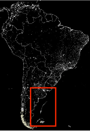
Figure 4: Fishing vessels off the coast of Argentina, http://subdude-site.com/WebPics/WebPicsEarthLights/south-america-hilights-429x600.jpg courtesy of Ricardo Matano, COAS, Oregon State University

The equation for the free surface elevation $\eta$ as a function of spatial variables $(x,y)$ is derived from principles of geostrophic balance and takes the form

(2.1) $${\partial\eta\over\partial y}=-{r\over f}\left({\partial h\over\partial x}\right)^{-1}{\partial^{2}\eta\over\partial x^{2}},$$

where $r>0$ and $f<0$ in the southern hemisphere, and $h(x)$ is the depth of the ocean at a distance $x$ from the shore. In particular, the sharp break in the shelf makes $h^{\prime}(x)$ a piecewise constant function with positive values $H^{+},H^{-}$. The location of the interface coincides with the distance to the shelf-break. In particular, if the spatial variable $y>0$ is viewed as a ‘time’ parameter, then this is a skew-diffusion equation, but the physics imply continuity of the derivatives $\partial\eta/\partial x$ at the interface rather than ‘flux’ (see [27] and references therein).

Example C (Fender’s Blue Butterfly). The Fenders Blue is an endangered species of butterfly found in the pacific northwestern United States. The primary habitat patch is Kinkaid’s Lupin flower (Figure 5).

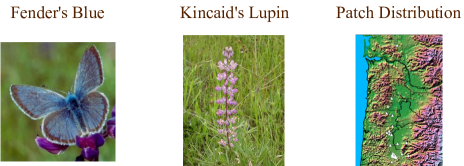
Figure 5: Fender’s Blue Butterfly Habitat - Kincaid’s Lupin Patches - U.S. Fish and Wildlife Service,Wikipedia http://en.wikipedia.org/wiki/Fender%27s_blue_butterfly, http://www.fws.gov/oregonfwo/Species/PrairieSpecies/gallery.asp

Quoting [44], “Given past research on the Fender’s blue, and the potential to investigate response to patch boundaries, we ask two central questions. First, how do organisms respond to habitat edges? Second, what are the implications of this behavior for residence times?” Sufficiently long residence (occupation) times in Lupin patches are required for pollination, eggs, larvae and ultimate sustainability of the population. Empirical evidence points to a skewness in random walk models for butterfly movement at the path boundaries. The determination of proper interface conditions is primarily a statistical problem in this application, however we will see that certain theoretical qualitative analysis may be possible for setting ranges on interface transmission parameters. There is a rapidly growing literature on the statistical estimation of parameters for diffusions, [28], [43], [1]. However much (though not all) of this literature is motivated by applications to dispersive models in finance for which the coefficients are presumed smooth and the data is high frequency.

Example D (Sustainability on a River Network). The movement of larvae in a river system is often modeled by advective-dispersion equations in which the rates are determined by hydrologic/geomorphologic relationships in the form of the so-called Horton laws. In general river networks (Figure 6) are modeled as directed binary tree graphs and each junction may be viewed as an interface. There are also special relations known from geomorphology and hydrology that can be applied to narrow the class of graphs observed in natural river basins; e.g., see [42], [34], [14], and references therein.

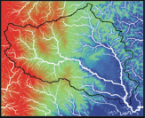
Figure 6: Digitally Generated River Network Using HidroSIG Java; courtesy of Jorge Ramirez

Conservation of mass leads to continuity of flux of larvae across each stream junction as the appropriate interface condition. Problems on sustainability in this context are generally formulated in terms of network size and characteristics relative to the production of larvae sufficient to prevent permanent downstream removal at low population sizes; see [40] for recent results in the case of a river network, and [30] and [18] for related mathematical considerations.

3 Natural Dispersion and Natural Occupation Time

The following theorem provides a useful summary in one-dimension of the interplay between diffusion coefficients and broader classes of possible interfacial conditions. To set the stage we begin with Brownian motion $X=\{X(t)\equiv\sqrt{D}B(t)+vt:t\geq 0\}$ with constant diffusion coefficient $D>0$ and constant drift $v$; i.e., $B=\{B(t):t\geq 0\}$ is standard Brownian motion starting at zero, with unit diffusion coefficient and zero drift. The stochastic process $X$ has a number of properties characteristic of diffusion. Namely, the random path $t\to X(t)$ is continuous with probability one, and

(3.1) $$\mathbb{E}(X(t)|X(u),u\leq s)=X(s)+v(t-s),\qquad 0\leq s<t.$$

This makes $X$ a continuous semimartingale. In the case $v=0$, $X$ is in fact said to be a (continuous) martingale. In general a continuous semimartingale is a process with continuous paths that differs from a (local) martingale by a (unique) continuous (adapted) process having finite total variation (in the sense of functions of bounded variation). Such structure is a natural consequence of the interfaces discussed in this article. This will be made clear at equation (3.12) below.

The Brownian motion $X$ is also a Markov process with (homogeneous) transition probabilities

(3.2) $$p(t,x,y)={1\over\sqrt{2\pi Dt}}e^{-{(y-x-vt)^{2}\over 2Dt}},\qquad t\geq 0,$$

satisfying the advection-dispersion equation

(3.3) $${\partial p\over\partial t}={\partial\over\partial y}({D\over 2}{\partial p\over\partial y})-{\partial vp\over\partial y}.$$

with continuous derivatives of all orders everywhere. Since the displacements $X(t)-X(s)$ are independent for disjoint intervals $(s,t)$, it follows that the variance of $X(t)$ is linear in $t$ and, in particular, $\mathbb{E}(X(t)-vt)^{2}=Dt,t\geq 0.$ The definition of mathematical local time at $a$, denoted $\ell_{t}^{X}(a)$, for $X$ can be expressed as $d\ell_{t}^{X}(a)$ is the amount of time $X$ spends in the infinitesimal neighborhood $(a,a\pm da)$ prior to time $t$. More precisely,

(3.4) $$\ell^{X}_{t}(a)=\lim_{\epsilon\downarrow 0}{D\over 2\epsilon}\int_{0}^{t}1_{(a-\epsilon,a+\epsilon)}(X(s))ds.$$

Note the presence of the diffusion coefficient $D$. Thus, in the context of dispersion of particles in a fluid, for example, $[D]=L^{2}/T$ and $[\epsilon]=[X]=L$ yields units $[\ell_{t}^{X}]={1\over L}\times{L^{2}\over T}\times T=L.$

The standard extension of the mathematical definition of local time for a continuous semimartingale $X$ exploits the quadratic variation $<X>_{t},t\geq 0,$ of the process. If $X$ is a square-integrable martingale then $<X>_{t}$ is defined by the property that the process $X^{2}(t)-<X>_{t},t\geq 0,$ is a martingale; see [41]. So, in the case of the Brownian motion one may check that $<X>_{t}=Dt,t\geq 0.$ In the case of a continuous semimartingale, the quadratic variation is quadratic variation of its martingale component.

Mathematical local time at $a$ can be defined as an increasing continuous stochastic process $\ell_{a}^{X}(t),t\geq 0$ such that

(3.5) $$|X(t)-a|=|X(0)-a|+\int_{0}^{t}{\text{s}gn}(X(s)-a)dX(s)+\ell_{t}^{X}(a),\qquad t\geq 0,$$

where ${\text{s}gn}(x)=x/|x|,x\neq 0,$ and ${\text{s}gn}(0)=-1$ (by convention). For purposes of calculation it is often convenient to consider (right and left) one-sided versions defined by

(3.6) $$\ell_{t}^{X,+}(a)=\lim_{\epsilon\downarrow 0}{1\over\epsilon}\int_{0}^{t}1_{[a,a+\epsilon)}(X(s))d<X>_{s},\qquad t\geq 0,$$

(3.7) $$\ell_{t}^{X,-}(a)=\lim_{\epsilon\downarrow 0}{1\over\epsilon}\int_{0}^{t}1_{(a-\epsilon,a]}(X(s))d<X>_{s},\qquad t\geq 0.$$

Then

(3.8) $$\ell_{t}^{X}(a)={\ell_{t}^{X,+}(a)+\ell_{t}^{X,-}(a)\over 2},\qquad t\geq 0.$$

The utility of these quantities rests in the following two formulae:

Itô-Tanaka Formula: If $X$ is a continuous semimartingale with local time $\ell_{t}^{X}(a),a\in\mathbb{R},t\geq 0$, and $f$ is the difference of two convex functions then

(3.9) $$f(X(t))=f(X(0))+\int_{0}^{t}f_{-}^{\prime}(X(s))dX(s)+{1\over 2}\int_{\mathbb{R}}\ell_{t}^{X,+}(a)f^{\prime\prime}(da),$$

where $f^{\prime\prime}(da)$ is a positive measure corresponding to the second derivative of $f$ in the sense of distributions.

Occupation Time Formula: For a non-negative Borel function $g$ and $t\geq 0$, one has a.e. that

(3.10) $$\int_{0}^{t}g(X(s))d<X>_{s}=\int_{\mathbb{R}}g(a)d\ell_{t}^{X}(a).$$

Theorem 3.1.

Let $D^{+},D^{-}$ be arbitrary positive numbers and let $0<\alpha,\lambda<1$. Define $Y^{(\alpha)}(t)=\sigma(B_{t}^{(\alpha)}),t\geq 0$, where $B^{(\alpha)}$ is skew Brownian motion with transmission parameter $\alpha$ and $\sigma(x)=\sqrt{D^{+}}x1_{[0,\infty)}(x)+\sqrt{D^{-}}x1_{(-\infty,0]}(x),\ x\in{\mathbb{R}}$. Then

$$M(t)=f(Y^{(\alpha)}(t))-{1\over 2}\int_{0}^{t}D(Y^{(\alpha)}(u))f^{\prime\prime}(Y(u))du,\quad t\geq 0,$$

is a martingale for all $f\in{\cal D}_{\lambda}=\{f\in C^{2}({\mathbb{R}}\backslash\{0\})\cap C({\mathbb{R}}):\lambda f^{\prime}(0^{+})=(1-\lambda)f^{\prime}(0^{-})\}$ if and only if

$$\alpha=\alpha(\lambda)={\lambda\sqrt{D^{-}}\over\lambda\sqrt{D^{-}}+(1-\lambda)\sqrt{D^{+}}}.$$

Proof.

In the case of skew Brownian motion one has the following relationships between mathematical local time at zero and its one-sided variants, e.g., see [31]

(3.11) $$\ell_{t}^{B^{(\alpha),+}}(0)=2\alpha\ell_{t}^{B^{(\alpha)}}(0),\qquad\ell_{t}^{B^{(\alpha),-}}(0)=2(1-\alpha)\ell_{t}^{B^{(\alpha)}}(0),\quad t\geq 0.$$

Moreover, $B^{(\alpha)}$ is the unique strong solution to the stochastic differential equation, see [22],

(3.12) $$dB^{(\alpha)}(t)={2\alpha-1\over 2\alpha}d\ell_{t}^{B^{(\alpha)},+}(0)+dB(t).$$

In particular, considering the integrated version, $B$ is the martingale component and ${2\alpha-1\over 2\alpha}\ell_{t}^{B^{(\alpha)}}$ is the finite variation component in the view of $B^{(\alpha)}$ as a semimartingale.

It is also straightforward to relate mathematical local times of $Y^{(\alpha)}$ and $B^{(\alpha)}$ through the one-sided formulae as:

$$\ell_{t}^{Y^{(\alpha)},+}(0)=\sqrt{D^{+}}\ell_{t}^{B^{(\alpha)},+}(0),\qquad\ell_{t}^{Y^{(\alpha)},-}(0)=\sqrt{D^{-}}\ell_{t}^{B^{(\alpha)},-}(0)$$

Applying the Itô-Tanaka formula to the positive and negative parts of $Y^{(\alpha)}$ together with (3.12), one has

$$d(Y^{(\alpha)}(t))^{+}=\sqrt{D^{+}}\{1_{[B^{(\alpha)}(t)>0]}dB(t)+{1\over 2}d\ell_{t}^{B^{(\alpha)},+}(0)\},$$

and

$$d(Y^{(\alpha)}(t))^{-}=\sqrt{D^{-}}\{-1_{[B^{(\alpha)}(t)\leq 0]}dB(t)-{(2\alpha-1)\over 2\alpha}d\ell_{t}^{B^{(\alpha)},+}(0)+{1\over 2}d\ell_{t}^{B^{(\alpha)},+}(0)\}.$$

Thus, since $Y^{(\alpha)}$ is the difference of its positive and negative parts and noting the cancellation, one has

(3.13) $$dY^{(\alpha)}(t)=\sqrt{D(B^{(\alpha)}(t))}dB(t)+\left(\frac{\sqrt{D^{+}}-\sqrt{D^{-}}}{2}+\sqrt{D^{-}}\frac{2\alpha-1}{2\alpha}\right)d\ell_{t}^{B^{(\alpha)},+}(0).$$

For a difference of convex functions $f\in{\cal D}_{\lambda}$,

$$f^{\prime\prime}(da)=f^{\prime\prime}(a)da+(f^{\prime}(0^{+})-f^{\prime}(0^{-})\delta_{0}(da).$$

With these preliminaries, again use the Itô-Tanaka theorem together with (3.11) and (3.13), to get

(3.14) $$f(Y^{(\alpha)}(t)) = f(Y^{(\alpha)}(0))+\int_{0}^{t}f_{-}^{\prime}(Y^{(\alpha)}(s))dY^{(\alpha)}(s)+{1\over 2}\int_{\mathbb{R}}\ell_{t}^{Y^{(\alpha)},+}(a)f^{\prime\prime}(da)$$

$$= f(Y^{(\alpha)}(0))+\int_{0}^{t}f_{-}^{\prime}(Y^{(\alpha)}(s))\sqrt{D(Y^{(\alpha)}(s))}dB(s)$$

$$+ {\alpha\sqrt{D^{+}}-(1-\alpha)\sqrt{D^{-}}\over 2\alpha}\int_{0}^{t}f_{-}^{\prime}(Y^{(\alpha)}(s))d\ell_{s}^{B^{(\alpha)},+}(0)$$

$$+ {1\over 2}\int_{\mathbb{R}}\ell_{t}^{Y^{(\alpha)},+}(a)f^{\prime\prime}(a)da$$

$$+ {1\over 2}\int_{\mathbb{R}}\ell_{t}^{Y^{(\alpha)},+}(a)(f^{\prime}(0^{+})-f^{\prime}(0^{-})\delta_{0}(da).$$

According to the mathematical occupation time formula relating mathematical occupation time and mathematical local time, and and noting that the quadratic variation is given by $d<Y^{(\alpha)}>_{s}=D(Y^{(\alpha)}(s))ds$, it also follows that

$${1\over 2}\int_{\mathbb{R}}f^{\prime\prime}(a)d\ell_{t}^{Y^{(\alpha)},+}(a)={1\over 2}\int_{0}^{t}D(Y^{(\alpha)}(s))f^{\prime\prime}(Y^{(\alpha)}(s))ds.$$

The asserted result now follows by subtracting this term from each side of the equation (3.14) and noting the cancellation of local time terms leaving a stochastic integral with respect to Brownian motion when and only when $\alpha=\alpha(\lambda)$, i.e.,

$${\alpha\sqrt{D^{+}}-(1-\alpha)\sqrt{D^{-}}\over 2\alpha}\int_{0}^{t}f_{-}^{\prime}(Y^{(\alpha)}(s))d\ell_{s}^{B^{(\alpha)},+}(0)+{1\over 2}\int_{\mathbb{R}}\ell_{t}^{Y^{(\alpha),+}}(a)(f^{\prime}(0^{+})-f^{\prime}(0^{-}))\delta_{0}(da)$$

$$= {\alpha\sqrt{D^{+}}-(1-\alpha)\sqrt{D^{-}}\over 2\alpha}f^{\prime}(0^{-})\ell_{t}^{B^{(\alpha)},+}(0)+{1\over 2}\sqrt{D^{+}}\ell_{t}^{B^{(\alpha)},+}(0)(f^{\prime}(0^{+})-f^{\prime}(0^{-}))$$

$$= [{\sqrt{D^{+}}\over 2}f^{\prime}(0^{+})-{1-\alpha\over 2\alpha}\sqrt{D^{-}}f^{\prime}(0^{-})]\ell_{t}^{B^{(\alpha)},+}(0)=0$$

if and only if ${1-\alpha\over\alpha}{\sqrt{D^{-}}\over\sqrt{D^{+}}}={1-\lambda\over\lambda}$. That this is enough follows from standard theory, e.g., Theorem 2.4 in [41]. ∎

Some implications for the examples will be described below in terms of the stochastic particle evolution, however one may also note that one has the following consequence at the scale of Kolmogorov’s backward equation.

Corollary 3.2.

Let $D^{+},D^{-}$ be arbitrary positive numbers and let $0<\alpha,\lambda<1$. Then for $c_{0}\in{\cal D}_{\lambda}$, the unique solution to

$${\partial c\over\partial t}={1\over 2}D(x){\partial^{2}c\over\partial x^{2}},\quad\lim_{t\to 0^{+}}c(t,x)=c_{0}(x),\quad\lambda{\partial c\over\partial x}(t,0^{+})=(1-\lambda){\partial c\over\partial x}(t,0^{-}),t>0,$$

is given by

$$c(t,x)=\mathbb{E}_{x}c_{0}(Y^{\alpha(\lambda)}(t)),\quad t\geq 0.$$

It is illuminating to consider Theorem 3.1 in the context of the examples.

Example A. Theorem 3.1 provides a generalization of the results obtained in [37] and [3] for the case of advection-dispersion problems across an interface described in Example A. One may check that

(3.15) $$\lambda={D^{+}\over D^{+}+D^{-}},\qquad\alpha^{*}={\sqrt{D^{+}}\over\sqrt{D^{+}}+\sqrt{D^{-}}}.$$

follow from Theorem 3.1 for this application. This coincides with the results of [37] and [3] obtained by other methods.

The following definition is made with reference to both the diffusion coefficient and the interface parameter in the context of this and the other examples.

Definition 3.3.

With the choice of $\alpha\equiv\alpha(\lambda)$ given by Theorem 3.1, we refer to the process $Y^{(\alpha(\lambda))}$ as the natural diffusion corresponding to the dispersion coefficients $D^{+},D^{-}$ and interface parameter $\lambda$.

Additional Nomenclature: We sometimes refer to the natural diffusion corresponding to $\lambda={D^{+}\over D^{+}+D^{-}},\alpha^{*}={\sqrt{D^{+}}\over\sqrt{D^{+}}+\sqrt{D^{-}}}$ as the physical diffusion. We refer to the diffusion in the case $\lambda=1/2,\alpha^{\sharp}={\sqrt{D^{-}}\over\sqrt{D^{+}}+\sqrt{D^{-}}}=1-\alpha^{*}$ as the Stroock-Varadhan diffusion since it is the solution to the particular martingale problem originating with these authors; see [45].

Example B. Observe that in the application to the coastal up-welling problem one obtains

(3.16) $$\lambda=1/2,\qquad\alpha(1/2)=\alpha^{\sharp}={\sqrt{D^{-}}\over\sqrt{D^{+}}+\sqrt{D^{-}}}.$$

The interface parameter provides continuity of the derivative, rather than of the flux, at the interface. The natural diffusion for this example may be checked to coincide with the Stroock-Varadhan diffusion in this case. Note that the answer to the first passage time problem will be exactly opposite to that obtained for the advection-dispersion experiments of Example A under this model.

The following modification of the usual notion of mathematical occupation time, where the integration is with respect to quadratic variation and in units of squared-length, provides a quantity in units of time that we refer to as natural occupation time.

Definition 3.4.

Let $X$ be a continuous semimartingale. The natural occupation time of $G$ by time $t$, is defined by $\tilde{\Gamma}(G,t)=\int_{0}^{t}1(X(s)\in G)ds,t\geq 0,$ for an arbitrary Borel subset $G$ of $\mathbb{R}$.

The following result illustrates another way in which the issue raised in Example B relating interfacial conditions to residence times is indeed a sensitive problem. The proof exploits the property of skew Brownian motion that for any $t>0$,

(3.17) $$P(B^{(\alpha)}>0)=\alpha.$$

This is easily checked from definition and, intuitively, reflects the property that the excursion interval $J_{n(t)}$ of $|B|$ containing $t$ must result in a $[A_{n(t)}=+1]$ coin flip, an event with probability $\alpha$.

Theorem 3.5.

Let $Y^{(\alpha(\lambda))}$ denote the natural diffusion for the dispersion coefficients $D^{+},D^{-}$ and interface parameter $\lambda$. Denote natural occupation time processes by

$$\tilde{\Gamma}_{\lambda}^{+}(t)=\int_{0}^{t}1[Y^{(\alpha(\lambda))}(s)>0]ds,\quad t\geq 0.$$

Similarly let $\tilde{\Gamma}_{\lambda}^{-}(t)=t-\tilde{\Gamma}_{\lambda}^{+}(t),t\geq 0.$ Then,

$$\mathbb{E}\tilde{\Gamma}_{\lambda}^{+}(t)>\mathbb{E}\tilde{\Gamma}_{\lambda}^{-}(t)\ \forall t>0\quad{\iff}\lambda>{\sqrt{D^{+}}\over\sqrt{D^{+}}+\sqrt{D^{-}}},$$

with equality when $\lambda={\sqrt{D^{+}}\over\sqrt{D^{+}}+\sqrt{D^{-}}}$.

Proof.

Using the definition of natural diffusion $Y^{(\alpha(\lambda))}$ for the parameters $D^{\pm},\lambda$ and the above noted property (3.17) of skew Brownian motion, one has

$$\mathbb{E}\tilde{\Gamma}_{\lambda}^{+}(t) := \mathbb{E}\int_{0}^{t}1[Y^{(\alpha(\lambda))}(s)>0]ds$$

$$= \mathbb{E}\int_{0}^{t}1[\sqrt{D^{+}}B^{(\alpha(\lambda))}(s))>0]ds$$

$$= \int_{0}^{t}P(B^{(\alpha(\lambda))}(s)>0)ds$$

$$= t\alpha(\lambda).$$

Similarly $\mathbb{E}\tilde{\Gamma}_{\lambda}^{-}(t)=t(1-\alpha(\lambda))$. Thus

$${\mathbb{E}\tilde{\Gamma}_{\lambda}^{+}(t)\over\mathbb{E}\tilde{\Gamma}_{\lambda}^{-}(t)}=({\alpha(\lambda)\over 1-\alpha(\lambda)})=({\lambda\sqrt{D^{-}}\over(1-\lambda)\sqrt{D^{+}}}).$$

The assertion now follows. ∎

Example A vs Example C. As noted previously, in the Example C pertaining to insect movement, the determination of an interface condition is largely a statistical issue as there is no scientific rationale to apply mass conservation principles, or smooth Fickean flux laws. In fact, it is interesting to observe that under the mass conservation one arrives at the interface parameter

(3.18) $$\lambda=D^{+}/(D^{+}+D^{-}),$$

for which the residence time is longer on average in the region with the faster dispersion rate! While this is to be anticipated for physical experiments of dispersion in porous media of the type described in Example A, Theorem 3.5 shows that in fact the conservative interface condition (defined by this choice of $\lambda$) would not be appropriate for models of animal movement for which the faster dispersion occurs in more hostile environments; e.g., see [26], [12], [32] for relevant considerations. There is indeed something to be learned from data as to what exactly might apply, but such theoretical insights can provide a useful guide, and help to prevent mistaken assumptions when transferring more well-developed physical principles to biological/ecological phenomena.

4 Continuity of Natural Local Time

We now discuss another issue pertaining to the definition of mathematical local time and the basis for the suggested modification to natural local time.

In the often cited article [47], it was first observed that skew-Brownian motion provides a non-trivial example of a continuous semimartingale on the interval $(-\infty,\infty)$ having a discontinuous mathematical local time. Let us now examine this situation in the context of natural diffusions. For the purposes of this discussion take the drift $v=0$ and consider a constant diffusion coefficient $D^{+}=D^{-}=D$

Since the quadratic variation of skew Brownian motion coincides with that of Brownian motion, one has $<\sqrt{D}B^{(\alpha)}>\equiv<\sqrt{D}B>.$ Among this class of natural diffusions, one may ask what distinguishes the particular diffusion $X\equiv\sqrt{D}B$ ? Of course, the answer is that $X$ is determined by $\alpha=\lambda=1/2$. If one views this choice in the context of the flux in particle concentration, then it provides continuity of flux. On the other hand, in view of the respective theorems of Trotter [46] and Walsh [47], it is also the unique choice of $\alpha$ from among all skew Brownian motions to make local time continuous. The latter may be viewed as a stochastic particle determination of the physical diffusion model, among natural diffusions, for constant diffusion coefficient $D$.

The next theorem, a version of which was originally conceived in [4], extends this to the more general framework of the present paper, in particular to include the case $D^{+}\neq D^{-}$. However, it requires the following modification of the definition of mathematical local time, referred to here as natural local time.

Definition 4.1.

Let $X$ be a continuous semimartingale. The natural local time at $a$ $\tilde{\ell}_{t}^{X}={\tilde{\ell}_{t}^{X,+}+\tilde{\ell}_{t}^{X,-}\over 2}$ of $X$ is defined by

(4.1) $$\tilde{\ell}_{t}^{X,+}(a)=\lim_{\epsilon\downarrow 0}{1\over\epsilon}\int_{0}^{t}1_{[a,a+\epsilon)}(X(s))ds,\quad\tilde{\ell}_{t}^{X,-}(a)=\lim_{\epsilon\downarrow 0}{1\over\epsilon}\int_{0}^{t}1_{(a-\epsilon,a]}(X(s))ds$$

providing the indicated limits exist almost surely.

The units of natural local time are then $[\tilde{\ell}_{t}^{X}]={T\over L}$, appropriate to a measurement of (occupation) time in the vicinity of a spatial location $a$. While the purpose here is not to explore the generality for which natural local time exists among all continuous semimartingales, according to the following theorem it does exist for natural skew diffusion. Moreover, continuity has a special significance.

Theorem 4.2.

Let $Y^{(\alpha(\lambda))}$ be the natural skew diffusion with parameters $D^{\pm},\lambda$. Then the natural local time of $Y^{(\alpha(\lambda))}$ at $0$ is continuous if and only if $\lambda={D^{+}\over D^{+}+D^{-}}$, i.e., if and only if $\alpha(\lambda)=\alpha^{*}$ and thus $Y^{(\alpha^{*})}$ is the physical diffusion.

Proof.

In view of (3.11) observe that

$${\ell_{t}^{B^{(\alpha)},+}(0)\over\ell_{t}^{B^{(\alpha)},-}(0)}={\alpha\over 1-\alpha},\qquad\forall t\geq 0.$$

Moreover,

$$\tilde{\ell}_{t}^{B^{(\alpha)},+}(0) = \lim_{\epsilon\downarrow 0}{1\over\epsilon}\int_{0}^{t}1[0\leq Y^{(\alpha)}(s)<\epsilon]ds$$

$$= {1\over\sqrt{D^{+}}}\lim_{\epsilon\downarrow 0}{\sqrt{D^{+}}\over\epsilon}\int_{0}^{t}1[0\leq B^{(\alpha)}(s)<{\epsilon\over\sqrt{D^{+}}}]ds$$

$$= {1\over\sqrt{D^{+}}}\ell_{t}^{B^{(\alpha)},+}(0).$$

Similarly, $\tilde{\ell}_{t}^{B^{(\alpha)},-}(0)={1\over\sqrt{D^{-}}}\ell_{t}^{B^{(\alpha)},-}(0).$ Thus,

$${\tilde{\ell}_{t}^{B^{\alpha(\lambda)},+}(0)\over\tilde{\ell}_{t}^{B^{\alpha(\lambda)},-}(0)}={\alpha(\lambda)\over 1-\alpha(\lambda)}{\sqrt{D^{-}}\over\sqrt{D^{+}}}.$$

Now simply observe that this ratio is one if and only if $\lambda D^{-}=(1-\lambda)D^{+}$, which establishes the assertion. ∎

5 Acknowledgments.

The authors are grateful to Jorge Ramirez for several technical comments that improved the content and exposition. The first author was partially supported by an NSF-IGERT-0333257 graduate training grant in ecosystems informatics at Oregon State University, and the remaining authors were partially supported by a grant DMS-1122699 from the National Science Foundation. The corresponding author is also grateful for support provided by the Courant Institute of Mathematical Sciences, New York University, during preparation of the final draft of this article.

References

- [1] A it-Sahalia,Y. (2008): Closed form likelihood expansions for multivariate diffusions, Ann. Statist. 36(2), 906-937.
- [2] Appuhamillage, T. (2011): The skew diffusion with drift: A new class of stochastic processes with applications to parabolic equations with piecewise smooth coefficients, PhD Thesis: Oregon State University, Corvallis, OR. USA.
- [3] Appuhamillage, T., V. Bokil, E. Thomann, E. Waymire, B. Wood (2011) Occupation and Local Times for Skew Brownian Motion with Applications to Dispersion Across an Interface, Annals of Appld. Probab, 21(1) 183–214. [Correction: Ann. Appld. Probab., to appear, http://arxiv.org/abs/1009.5410.]
- [4] Appuhamillage, T., V. Bokil, E. Thomann, E. Waymire, B. Wood (2009) Solute Transport Across an Interface: A Fickian Theory for Skewness in Breakthrough Curve, Water Resour. Res, 46, W07511, doi:10.1029/2009WR008258.
- [5] Appuhamillage, T.A., D. Sheldon (2012) First passage time of skew Brownian motion, Jour. Appld. Probab. (to appear) http://arxiv.org/pdf/1008.2989
- [6] Ben Arous, G., A. F. Ramirez (2000): Asymptotic survival probabilities in the random saturation process, Ann. Probab. 4(28), 1470-1527.
- [7] Berkowitz, B., A. Cortis, I. Dror, and H. Scher (2009), Laboratory experiments on dispersive transport across interfaces: The role of flow direction, Water Resour. Res., 45, W02201, doi:10.1029/2008WR007342.
- [8] Bhattacharya, R., V.K. Gupta Solute dispersion in multidimensional periodic porous media (1986) Water Res. Research, 22(2), 156-164
- [9] Bhattacharya, R.N., F. Götze (1994): Time scales for Gaussian approximation and its breakdown under a hierarchy of periodic spatial heterogeneities, Bernoulli 1, 81-123
- [10] Bhattacharya, R. N. (1999): Multiscale diffusion processes with periodic coefficients and an application to solute transport in porous media. (Special Invited Paper), Annals of Applied Probability, 9 951-1020.
- [11] Bhattacharya, R.N., E. Waymire (1990), Stochastic Processes with applications, Wiley, NY. [Reprinted in the SIAM Classics in Applied Mathematics book series, 2009.]
- [12] Cosner, C.C., R.S. Cantrell (2003): Spatial ecology via reaction- diffusion equations, Wiley, NY.
- [13] Cushman, J.H., L.S. Bennethum* and B.X. Hu* (2002) A primer on upscaling methods for porous media. Adv. Water Resour. 25 1043-1067
- [14] Gupta, V.K., R. Mantilla, B.M. Troutman, D. Dawdy, W.F. Krajewski (2010): Generalizing a geophysical flood theory to medium-sized river networks, Geophys. Res. Lett. 37 L11402
- [15] Durrett, R., M. Restrepo (2008): One-dimensional stepping stone models, sardine genetics and Brownian local time, Annals of Applied Probab. 18(1), 334-358.
- [16] Einstein, A. (1905): Die von der Molekularkinetischen Theorie der Wärme Gefordete Bewegung von in ruhenden Flüssigkeiten Suspendierten Teilchen, Ann. Phys. 17 549-560.
- [17] Eisenbaum, N., and H. Kaspi (2007) On the continuity of local times of Borel right Markov processes, Ann. Probab. 35(3), 915-934.
- [18] Friedlin, M., Sheu, J.S. (2000): Diffusion processes on graphs: stochastics differential equations, large deviation principle, Probability Theory and Related Fields, 116 181-220.
- [19] Harrison, J.M. and L. A. Shepp, On skew Brownian motion, Ann. Probab., 9 (1981), pp. 309–313.
- [20] Hoteit, H., R. Mose, A. Younes, F. Lehmann, Ph. Ackerer (2002), Three-dimensional modeling of mass transfer in porous media using the mixed hybrid finite elements and random walk methods, Mathematical Geology, 34(4), 435-456.
- [21] Itô, K. and H. P. McKean, Brownian motions on a half line, Illinois J. Math., 7 (1963), pp. 181–231.
- [22] Le Gall, J.-F. One-dimensional stochastic differential equations involving the local times of the unknown process. Stochastic analysis and applications (Swansea, 1983), 51–82, Lecture Notes in Math., 1095, Springer, Berlin, 1984
- [23] Kuo, R. K. H. and Irwin, N. C. and Greenkorn, R. A. and Cushman, J. H. (1999), Experimental investigation of mixing in aperiodic heterogeneous porous media: Comparison with stochastic transport theory, Transport in Porous Media, 37, 169-182.
- [24] LaBolle, E.M., J. Quastel, Graham E. Fogg, and J. Gravner: Diffusion processes in composite porous media and their numerical integration by random walks: Generalized stochastic differential equations with discontinuous coefficients, Water Resour. Res. (2000) 36(3), 651-662.
- [25] Lejay, A., M. Martinez (2008), A scheme for simulating one-dimensional diffusion processes with discontinuous coefficients, Ann. Appld. Probab. 116(1), 107-139.
- [26] McKenzie, H.W., M.A. Lewis, and E.H. Merrill (2009), First passage time analysis of animal movement and insights into functional response, Bull. Math. Bio. 71(1), 107–129.
- [27] Matano, Ricardo P., Elbio D. Palma. (2008), On the upwelling of downwelling currents, Jour. Phys. Ocean., 38(11) 2482–2500.
- [28] Nakahiro, Y. (1992): Estimation for diffusion from discrete observation, J. Multi. Anal. 41(2), 220-242.
- [29] Newburgh, R., J. Peidle, W. Rueckner (2006): Einstein, Perrin, and the reality of atoms: 1905 revisited, Am. J. Phys. 74(6) 478–481
- [30] Okada, T. (1993): Asymptotics behavior of skew conditional heat kernels on graph networks, Can. J. Math. 45(4), 863-878.
- [31] Ouknine, Y. (1991): Skew-Brownian motion and associated processes Theory Probab. Appl. 35 (1990), no. 1, 163–169.
- [32] Ovaskainen, O. (2004), Habitat-specific movement parameters estimated using mark-recapture data and a diffusion model, Ecology 85 242D257.
- [33] G. Papanicolaou, S. R. S. Varadhan, Boundary value problems with rapidly oscillating random coefficients, Coll. Math. Soc. J?anos Bolyai, 27 Random fields, (Esztergom, 1979) ,835-873 North-Holland, Amsterdam 1982.
- [34] Peckham, Scott (1995): New results for self-similar trees with applications to river networks, Water. Res. Res. 31(4), 1023-1029.
- [35] Perrin, J. (1909): Le Mouvement Brownien et la Rèalité Moleculaire, Ann. Chimi. Phys. 18 8me Serie, 5-114
- [36] Ramirez, J. (2007): Skew Brownian motion and branching processes applied to advective-diffusion in porous media and fluid flow, PhD Thesis, Oregon State University.
- [37] Ramirez, J., E. Thomann, E. Waymire, R. Haggerty, B. Wood (2006), A generalized Taylor-Aris formula and skew diffusion, SIAM Multiscale Modeling and Simulation 5 3, 786-801.
- [38] Ramirez, J. M., E. A. Thomann, E. C. Waymire, J. Chastanet, and B. D. Wood (2008), A note on the theoretical foundations of particle tracking methods in heterogeneous porous media, Water Resour. Res., 44, W01501, doi:10.1029/2007WR005914.
- [39] Ramirez, J.M. (2011), Multi-skewed Brownian motion and diffusion in layered media, Proceedings of the American Mathematical Society. 139 3739-3752.
- [40] Ramirez, J.M. (2011), Population persistence under advection-diffusion in river networks, Mathematical Biology DOI 10.1007/s00285-011-0485-6.
- [41] Revuz, Daniel, and Marc Yor (1999), Continuous martingales and Brownian motion Springer, NY.
- [42] Rinaldo, A., I. Rodriguez-Iturbe Fractal river basins: chance and self-organization
- [43] Sorensen, M. (2004): Martingale estimating functions for discretely observed stochastic differential equation models, In: Interplay between semigroups and PDEs: Theory and Application, eds., Romanelli, S., R.M. Minnini, and S. Lucente, Aracne Editrice, Rome, 213-236.
- [44] Schultz, Cheryl B., and Elizabeth E. Crone (2005), Patch size and connectivity thresholds for butterfly habitat restoration, Conservation Biology, 19(3), 887-896.
- [45] Stroock, Daniel, W., and S.R. Srinivasa Varadhan (1997), Multidimensional diffusion processes Springer, NY.
- [46] Trotter, H. (1958) A property of Brownian motion paths, Ill. J. Math. 2 425–433.
- [47] Walsh, J. (1978): A diffusion with a discontinuous local time, Asterisque, 52–53, pp. 37–45.
- [48] Winter, C. L., C. M. Newman and S. P. Neuman (1984). A perturbation expansion for diffusion in a random velocity field. SIAM J. Appl. Math., 44 411-424.