Computational science and re-discovery: open-source implementations of ellipsoidal harmonics for problems in potential theory

Abstract

We present two open-source (BSD) implementations of ellipsoidal harmonic expansions for solving problems of potential theory using separation of variables. Ellipsoidal harmonics are used surprisingly infrequently, considering their substantial value for problems ranging in scale from molecules to the entire solar system. In this article, we suggest two possible reasons for the paucity relative to spherical harmonics. The first is essentially historical—ellipsoidal harmonics developed during the late 19th century and early 20th, when it was found that only the lowest-order harmonics are expressible in closed form. Each higher-order term requires the solution of an eigenvalue problem, and tedious manual computation seems to have discouraged applications and theoretical studies. The second explanation is practical: even with modern computers and accurate eigenvalue algorithms, expansions in ellipsoidal harmonics are significantly more challenging to compute than those in Cartesian or spherical coordinates. The present implementations reduce the “barrier to entry” by providing an easy and free way for the community to begin using ellipsoidal harmonics in actual research. We demonstrate our implementation using the specific and physiologically crucial problem of how charged proteins interact with their environment, and ask: what other analytical tools await re-discovery in an era of inexpensive computation?

I Introduction

It is intuitively obvious that a cow is much better approximated by an ellipsoid than by a sphere. Less obvious, or at least less well known, is the method of ellipsoidal harmonics for solving the ellipsoidal cow exactly Hobson31 ; DassiosBook . In an effort to increase the popularity and impact of these fascinating functions, we present in this paper two open-source (BSD) implementations for calculating the ellipsoidal harmonics and solving problems of potential theory (they may be downloaded freely online bitbucket-ellipsoidal ). To demonstrate the methods’ correctness, we model the physiologically crucial electrostatic interactions between a protein and surrounding water using a popular continuum theory based on the Poisson equation Sharp90 ; Honig95 . Our results indicate, that improved numerical methods are needed, and we hope that releasing these codes will not only encourage application scientists to try ellipsoidal harmonics, but also motivate numerical analysts to help develop more accurate computational approaches.

Our implementations, written in Python and MATLAB Matlab , employ a variety of insights developed over more than a century of research Hobson31 ; Romain01 ; Xue11 ; many important results were published during the mid-19th century and early 20th by greats like Heine Heine78 , and Charles Darwin’s son Sir George Howard Darwin Darwin01 . From the authors’ perspective, these surprisingly direct ties to mathematical history offer an unusual and inspiring aspect to their study. Ellipsoidal coordinates are the most general coordinate system for which the Laplace equation is separable, as the other coordinate systems for which Laplace is separable can all be considered degenerate forms of ellipsoidal coordinates MorseFeshbach53 . In fact, the functions for each coordinate direction satisfy the same scalar equation, the Lamé equation. It seems somewhat ironic that the most general separable coordinate system should lead to this simple Cartesian-like result rather than to a more complicated form as found e.g. in spherical harmonics; the rabbit hole goes much deeper, but for now it suffices to observe that ellipsoidal harmonics are not a simple generalization of spherical harmonics.

Unsurprisingly, the more general shape allows ellipsoidal-harmonic expansions to be more accurate than ones based on spherical harmonics Stiles79 ; Romain01 ; Yu03 . Successful applications cover most of potential theory: gravity Darwin01 ; Romain01 , electrostatics Perram76 ; Rinaldi82 ; Rinaldi92 ; Ford92 ; Xue11 ; Kang07 , electromagnetics Dassios80 ; Dassios87 ; Dassios03 ; Kariotou04 , hydrodynamics Woessner62 ; Douglas95 ; Youngren75_2 ; Ryabov06 , and elasticity Ammari07 . Specific uses in molecular and biological sciences include solving the Schrödinger equation Levitina00 , modeling van der Waals (close packing) interactions between molecules Stiles79 , design of magnetic resonance imaging (MRI) devices Crozier02 and analysis of clinical electroencephalography (EEG) and magnetoencephalography (MEG) data Dassios03 ; Kariotou04 . Unfortunately, despite the range of applications and their advantages over spheres, a comparatively small number of publications actually use, or encourage the use of, ellipsoidal harmonics in practice. Notable and welcome exceptions may be found in Sten’s excellent tutorial review Sten06 and presumably in the upcoming book of Dassios DassiosBook , who has been one of the subject’s leading developers and champions Dassios80 ; Dassios02 ; Dassios03 ; Dassios09 ; Dassios09_2 . A few older books also address the theory Bowman ; Byerly , but for decades the authoritative reference has been E. W. Hobson’s 1931 text Hobson31 , published only two years before he passed away (for a charming obituary, see HobsonObituary ).

One reason for the relative dearth of papers using ellipsoidal harmonics is that they are hard to compute: unfortunately for investigators who might be interested in actually using ellipsoidal harmonics, widely available references do not address the numerous critical challenges associated with actually computing ellipsoidal harmonics to arbitrary order. Naïve numerical algorithms for their determination are unstable Sona95 , and careful reformulations are required Rinaldi82 ; Dobner97 ; Ritter98 ; Dobner98 ; Romain01 . This difficulty contrasts sharply to calculations in spherical harmonics or Cartesian space, where the functions for the expansion are given in closed form and can be computed easily. A second possible explanation, more speculative, is that the foundations of ellipsoidal harmonic analysis were developed many decades before the advent of digital computers Niven1891 ; Darwin01 ; Hobson31 ; actually using ellipsoidal harmonics to arbitrary order necessitates extensive computation, whether manual or by computer. Computation is necessary because the harmonics are defined as polynomials whose coefficients are solutions to eigenvalue problems. As such only the lowest-order modes can be expressed in closed form Hobson31 , and all other modes must be determined numerically (by the Abel-Ruffini theorem). Furthermore, the harmonics depend on the semi-axes of the ellipsoid, necessitating a new set of tedious manual computations for every problem. For that matter, we note that even the modes available in closed form require cumbersome algebraic manipulations Dassios03 ; Dassios09_2 . It seems that the large quantities of manual arithmetic led practitioners in many fields to adopt less accurate, but much more easily computed, spherical harmonic methods.

Thus, it seems possible that open-source implementations of ellipsoidal harmonics, based on the latest numerical algorithms for their computation, could encourage their re-discovery and wide application in computational science. The present work offers a simple demonstration that deriving an analytical solution using ellipsoidal harmonics is not any harder than deriving one using spherical harmonics. Instead, the challenge is in computing the functions themselves, a problem met by the released implementations; though, again, we acknowledge that a number of improvements are needed. We begin the technical portion of the paper in Section II, which presents the application setting (continuum electrostatics for biomolecular solvation) and the mathematical components needed to compute ellipsoidal harmonics. In Section III we describe our implementations at a high-level but highlight critical details and subtle issues. Section IV presents computational results, and Section V concludes the paper with a discussion of remaining challenges and possible future directions.

II Theory

Space constraints preclude full accounting of these topics; we present only the most relevant formulae and refer interested readers to the extensive and excellent treatments which have made our work possible Hobson31 ; Romain01 ; Dassios03 ; Xue11 . It is unfortunate that the clearest publications do not use a single, consistent notation; some types of analyses and identities are more readily seen in one notation or another. We have attempted to use the most popular conventions where possible, and apologize for introducing yet another mongrel notation.

II.1 Biomolecule Electrostatics

We assume that the biomolecule is a triaxial ellipsoid whose surface satisfies

$$\frac{x^{2}}{a^{2}}+\frac{y^{2}}{b^{2}}+\frac{z^{2}}{c^{2}}=1,$$ (1)

with $0<c<b<a<\infty$ called the ellipsoid’s semiaxes. In this paper, we use the term ellipsoid to mean a tri-axial ellipsoid (three unequal semi-axes), which is the most general ellipsoidal geometry. Ellipsoids with two equal semi-axes are called spheroids, these special cases are still more more straightforward to study Ahner86 ; Ahner94 ; Ahner94_2 ; Ahner96 ; Langebartel91 ; Martinec97 ; Jansen00 and apply AmbiaGarrido08 ; DiBiasio10 ; Frankel12 .

The molecular interior is assumed to be a homogeneous local dielectric of relative permittivity $\epsilon_{1}$ obeying linear response, and the molecular charge distribution is (without loss of generality) assumed to be a set of $Q$ discrete point charges, the $i$th of which being situated at ${\bf r}_{i}$ and having value $q_{i}$. Thus, inside the molecule (called region 1), the electrostatic potential obeys the Poisson equation

$$\nabla^{2}\Phi_{1}({\bf r})=-\frac{1}{\epsilon_{1}}\sum_{k=1}^{Q}q_{i}\delta({\bf r}-{\bf r}_{i})$$ (2)

where $\delta({\bf r})$ is the Dirac delta function. The solvent outside the molecule (region 2) is modeled as a homogeneous dielectric with dielectric constant $\epsilon_{2}$ and no fixed charges (i.e. we are modeling a salt-free solution), so the potential in this region obeys the Laplace equation

$$\nabla^{2}\Phi_{2}({\bf r})=0.$$ (3)

At the dielectric boundary, i.e., the ellipsoid surface defined by Eq. 1, the potential is continuous, as is the normal component of the electric displacement field $\mathbf{D}({\bf r})=\epsilon({\bf r})\mathbf{E}({\bf r})$, so for a point ${\bf r}_{S}$ on the surface,

$$\Phi_{1}({\bf r}_{S}) =\Phi_{2}({\bf r}_{S}))$$ (4)

$$\epsilon_{1}\frac{\partial\Phi_{1}}{\partial n}({\bf r}_{S}) =\epsilon_{2}\frac{\partial\Phi_{2}}{\partial n}({\bf r}_{S})$$ (5)

and we assume that the normal direction $\hat{\mathbf{n}}({\bf r}_{S})$ points outward into the solvent. The potential is assumed to decay sufficiently rapidly as $||{\bf r}||\rightarrow\infty$. We note that more sophisticated electrostatic models have been presented, e.g. Xue11 ; here we use a simple and popular one Sharp90 ; Honig95 to demonstrate our implementation.

II.2 Ellipsoidal Coordinates and Separation of Variables

In the ellipsoidal coordinate system, a point denoted in Cartesian space ${\bf r}=(x,y,z)$ is written as $(\lambda,\mu,\nu)$; each ellipsoidal coordinate is a root of the cubic

$$\frac{x^{2}}{s^{2}}+\frac{y^{2}}{s^{2}-h^{2}}+\frac{z^{2}}{s^{2}-k^{2}}=1$$ (6)

with

$$h^{2} =a^{2}-b^{2}$$ (7)

$$k^{2} =a^{2}-c^{2}$$ (8)

and we take the positive square roots so that $0<h<k$. The squares of the ellipsoidal coordinates are in the ranges

$$\lambda^{2} \in\left[k^{2},+\infty\right.\left.\right)$$ (9)

$$\mu^{2} \in\left[h^{2},k^{2}\right]$$ (10)

$$\nu^{2} \in\left[0,h^{2}\right].$$ (11)

Points on the surface of the ellipsoid with semi-axes $a$, $b$, and $c$ satisfy $\lambda=a$. Many texts enforce that $\lambda$ is positive, i.e. $\lambda\in\left[k,+\infty\right.\left.\right)$, by analogy with the radial coordinate in spherical systems. We have found non-negativity assumption problematic for inverse coordinate transforms and do not use it (see discussion in Sections III and V).

Our expressions for coordinate transformations come from Romain and Jean-Pierre Romain01 , who note that for a given point ${\bf r}=(x,y,z)$, the magnitudes of the ellipsoidal coordinates $(\lambda,\mu,\nu)$ can be computed via

$$\lambda^{2} =2\sqrt{Q}\cos\left(\frac{\theta}{3}\right)-\frac{w_{1}}{3}$$ (12)

$$\mu^{2} =2\sqrt{Q}\cos\left(\frac{\theta}{3}+\frac{4\pi}{3}\right)-\frac{w_{1}}{3}$$

$$\nu^{2} =2\sqrt{Q}\cos\left(\frac{\theta}{3}+\frac{2\pi}{3}\right)-\frac{w_{1}}{3}$$

where

$$Q =\frac{w_{1}^{2}-3w_{2}}{9}$$ (13)

$$R =\frac{9w_{1}w_{2}-27w_{3}-2w_{1}^{3}}{54}$$ (14)

$$\cos\theta =\frac{R}{\sqrt{Q^{3}}}$$ (15)

$$w_{1} =-(x^{2}+y^{2}+z^{2}+h^{2}+k^{2})$$ (16)

$$w_{2} =x^{2}(h^{2}+k^{2})+y^{2}k^{2}+z^{2}h^{2}+h^{2}k^{2}$$ (17)

$$w_{3} =-x^{2}h^{2}k^{2}.$$ (18)

The Cartesian coordinates can be computed from the ellipsoidal ones via

$$x^{2} =\frac{\lambda^{2}\mu^{2}\nu^{2}}{h^{2}k^{2}}$$ (19)

$$y^{2} =\frac{(\lambda^{2}-h^{2})(\mu^{2}-h^{2})(h^{2}-\nu^{2})}{h^{2}(k^{2}-h^{2})}$$

$$z^{2} =\frac{(\lambda^{2}-k^{2})(k^{2}-\mu^{2})(k^{2}-\nu^{2})}{k^{2}(k^{2}-h^{2})}$$

Romain and Jean-Pierre note that the simple Cartesian-to-ellipsoidal transformation of Eq. 12 suffers accuracy problems that can be important in special cases, and present a more sophisticated approach for improved accuracy Romain01 . Our present implementation includes only Eq. 12, and the improved algorithm is under development. All coordinate transformations using this simpler method are verified by computing the inverse transform and checking with a tolerance of $10^{-6}$. Also, we note that the above expressions correct a small typographical error in Eq. 7 of their work.

II.3 The Lamé Equation and its Solutions

In ellipsoidal harmonics, the Laplace equation separates such that the solutions for each coordinate satisfy the same differential equation (Eq. 20), which is called Lamé’s equation:

$$(s^{2}-h^{2})(s^{2}-k^{2})\frac{d^{2}E}{ds^{2}}(s)+s(2s^{2}-h^{2}-k^{2})\frac{dE}{ds}(s)+(p-qs^{2})E(s)=0$$ (20)

where $p$ and $q$ are unknown constants. It turns out that $q=n(n+1)$, and $p$ is an eigenvalue of a finite-dimensional matrix (see below).

The solutions of interest belong to four classes of polynomials, which are often labeled $\mathcal{K}(s)$, $\mathcal{L}(s)$, $\mathcal{M}(s)$, and $\mathcal{N}(s)$. For every nonnegative polynomial degree $n$, there are a total of $2n+1$ number of solutions from these classes. Specifically, defining $r=n/2$ for $n$ even and $r=(n-1)/2$ for $n$ odd, we have $r+1$ solutions in the class $\mathcal{K}_{n}(s)$, $n-r$ solutions in $\mathcal{L}_{n}(s)$, $n-r$ solutions in $\mathcal{M}_{n}(s)$, and $r$ in $\mathcal{N}_{n}(s)$. By analogy with spherical harmonics, these $2n+1$ solutions of degree $n$ are labeled $E_{n}^{p}(s)$, with $p$ (since it is individual to each solution) serving double duty as a dummy index from 0 to $2n+1$. Convention holds that these solutions are assembled class-by-class in alphabetical order, i.e. for $0\leq p\leq r$, $E_{n}^{p}(s)=\mathcal{K}_{n}^{p}(s)$, then the next $n-r$ are the solutions $\mathcal{L}_{n}^{p}(s)$, and so forth.

For brevity, we describe how to determine only one of the classes of solutions; Romain and Jean-Pierre include a complete and detailed description of all four Romain01 , and our software implementation discussed in Section III can be consulted for full details. A stable algorithm introduced by Dobner and Ritter Dobner97 ; Dobner98 ; Ritter98 begins by writing the solution class as

$$\mathcal{K}_{n}^{p}(s) =\psi_{n}^{\mathcal{K},p}(s)P_{n}^{\mathcal{K},p}(s)$$ (21)

with

$$\psi_{n}^{\mathcal{K},p}(s)=s^{n-2r}$$ (22)

and

$$P_{n}^{\mathcal{K},p}(s)=\sum_{j=0}^{r}b_{j}\left(1-\frac{s^{2}}{h^{2}}\right)^{j}.$$ (23)

The $p$th solution $\mathcal{K}_{n}^{p}(s)$ is determined by the coefficients $b_{j}$ in Eq. 23, which represent the $p$th eigenvector of a tridiagonal matrix of the form

$$\left[\begin{array}[]{cccccc}\tilde{d}_{0}&\tilde{g}_{0}&0&0&\cdots&0\\ \tilde{f}_{1}&\tilde{d}_{1}&\tilde{g}_{1}&0&\cdots&0\\ 0&\tilde{f}_{2}&\tilde{d}_{2}&\tilde{g}_{2}&\cdots&0\\ 0&&&&\ddots&\vdots\\ 0&0&\cdots&0&\tilde{f}_{r}&\tilde{d}_{r}\end{array}\right],$$ (24)

where the nonzero elements $\tilde{f}_{i}$, $\tilde{d}_{i}$, and $\tilde{g}_{i}$ depend on the solution class, the ellipsoid semi-axes, $n$, and $r$.

The above solutions are known as Lamé functions of the first kind; they diverge as $s\rightarrow\infty$, making it impossible to write solutions to the Laplace equation in exterior regions using these functions. A closely related set of solutions do behave appropriately in this limit, and are known as Lamé functions of the second kind; these only involve the radial-like coordinate $\lambda$ and are written

$$F_{n}^{p}(\lambda)=(2n+1)E_{n}^{p}(\lambda)I_{n}^{p}(\lambda)$$ (25)

where

$$I_{n}^{p}(\lambda)=\int^{\infty}_{\lambda}\frac{ds}{\left[E_{n}^{p}(s)\right]^{2}\sqrt{s^{2}-k^{2}}\sqrt{s^{2}-h^{2}}}.$$ (26)

II.4 Ellipsoidal Harmonics

For a given degree $n$ and order $p$, the interior solid ellipsoidal harmonic is defined as

$$\mathbb{E}_{n}^{p}(\lambda,\mu,\nu)=E_{n}^{p}(\lambda)E_{n}^{p}(\mu)E_{n}^{p}(\nu),$$ (27)

the exterior solid ellipsoidal harmonic as

$$\mathbb{F}_{n}^{p}(\lambda,\mu,\nu)=(2n+1)\mathbb{E}_{n}^{p}(\lambda,\mu,\nu)I_{n}^{p}(\lambda),$$ (28)

and the surface ellipsoidal harmonic as

$$\mathcal{E}_{n}^{p}(\mu,\nu)=E_{n}^{p}(\mu)E_{n}^{p}(\nu).$$ (29)

The surface harmonics satisfy the orthogonality condition

$$\int\int_{\lambda=a}\mathcal{E}_{n}^{p}(\mu,\nu)\mathcal{E}_{n^{\prime}}^{p^{\prime}}(\mu,\nu)ds=\gamma_{n}^{p}\delta_{nn^{\prime}}\delta_{pp^{\prime}}$$ (30)

where $\gamma_{n}^{p}$ is a normalization constant; writing the surface integral more explicitly,

$$\gamma_{n}^{p}=\int_{0}^{h}\int_{h}^{k}\left(\mathcal{E}_{n}^{p}(\mu,\nu)\right)^{2}\frac{(\mu^{2}-\nu^{2})}{\sqrt{(\mu^{2}-h^{2})(k^{2}-\mu^{2})}\sqrt{(h^{2}-\nu^{2})(k^{2}-\nu^{2})}}d\mu\;d\nu.$$ (31)

Then the Coulomb potential at ${\bf r}$ due to a unit charge at ${\bf r}^{\prime}$ (with $||{\bf r}||>||{\bf r}^{\prime}||$) is expanded in ellipsoidal harmonics as

$$\frac{1}{||{\bf r}-{\bf r}^{\prime}||}=\sum_{n=0}^{\infty}\sum_{p=1}^{2n+1}\frac{4\pi}{2n+1}\frac{1}{\gamma_{n}^{p}}\mathbb{E}_{n}^{p}({\bf r}^{\prime})\mathbb{F}_{n}^{p}({\bf r}),$$ (32)

or a similar form if $||{\bf r}||<||{\bf r}^{\prime}||$ (see, e.g., Xue11 ). The normal derivative at the ellipsoid surface defined by $\lambda=a$ is computed as Dassios03

$$\frac{\partial}{\partial n}=\hat{\mathbf{\lambda}}\cdot\nabla=\frac{bc}{\sqrt{a^{2}-\mu^{2}}\sqrt{a^{2}-\nu^{2}}}\frac{\partial}{\partial\lambda}$$ (33)

II.5 Series Solution for Biomolecule Electrostatics

In analogy with the Kirkwood series solution for a spherical particle Kirkwood34 , we formulate our model problem in ellipsoidal coordinates ${\bf r}=(\lambda,\mu,\nu)$. The potential in region 1, $\Phi_{1}({\bf r})$, can be written

$$\Phi_{1}({\bf r})=\sum^{Q}_{k=1}\frac{q_{k}}{\epsilon_{1}\left|{\bf r}-{\bf r}_{k}\right|}+\psi({\bf r}),$$ (34)

where $\psi({\bf r})$ is the reaction potential. We expand $\psi$ in ellipsoidal harmonics of the first kind (interior harmonics) since these are valid within region 1:

$$\psi({\bf r})=\sum^{\infty}_{n=0}\sum^{2n+1}_{p=1}B_{n}^{p}\;\mathbb{E}^{p}_{n}({\bf r}).$$ (35)

Similarly, the potential in region 2 may be expanded in ellipsoidal harmonics of the second kind (exterior harmonics), which are regular as $||{\bf r}||\rightarrow\infty$:

$$\Phi_{2}({\bf r})=\sum^{\infty}_{n=0}\sum^{2n+1}_{p=1}C_{n}^{p}\;\mathbb{F}^{p}_{n}({\bf r}).$$ (36)

To determine the constants appearing in these expansions, we apply the boundary conditions Eqs. (4) and (5) by relating them to the Coulomb portion of $\Phi_{1}$, using the fact that all charges are contained inside the ellipsoid ($\lambda_{k}<\lambda$). Using the Coulomb-potential expansion from Eq. 32,

$$\sum^{Q}_{k=1}\frac{q_{k}}{\epsilon_{1}\left|{\bf r}-{\bf r}_{k}\right|} = \sum^{Q}_{k=1}\frac{q_{k}}{\epsilon_{1}}\sum^{\infty}_{n=0}\sum^{2n+1}_{p=1}\frac{4\pi}{2n+1}\frac{1}{\gamma^{p}_{n}}\mathbb{F}^{p}_{n}({\bf r})\mathbb{E}^{p}_{n}({\bf r}_{k})$$ (37)

$$= \sum^{\infty}_{n=0}\sum^{2n+1}_{p=1}\frac{G_{n}^{p}}{\epsilon_{1}}\mathbb{F}^{p}_{n}({\bf r})$$ (38)

where

$$G_{n}^{p}=\sum^{Q}_{k=1}q_{k}\frac{4\pi}{2n+1}\frac{1}{\gamma^{p}_{n}}\mathbb{E}^{p}_{n}({\bf r}_{k}).$$ (39)

Now the first boundary condition, Eq. (4), gives us, after equating each $(n,p)$ term in order for the relation to hold for all angles,

$$\frac{G_{n}^{p}}{\epsilon_{1}}+B_{n}^{p}\frac{\mathbb{E}^{p}_{n}({\bf r}_{S})}{\mathbb{F}^{p}_{n}({\bf r}_{S})} = C_{n}^{p}$$ (40)

$$\frac{G_{n}^{p}}{\epsilon_{1}}+B_{n}^{p}\frac{E^{p}_{n}(a)}{F^{p}_{n}(a)} = C_{n}^{p}$$ (41)

In order to apply Eq. (5), we differentiate each series term by term and equate them,

$$\frac{G_{n}^{p}}{\epsilon_{2}}+\frac{\epsilon_{1}}{\epsilon_{2}}\frac{\frac{\partial\mathbb{E}^{p}_{n}({\bf r})}{\partial\lambda}|_{a}}{\frac{\partial\mathbb{F}^{p}_{n}({\bf r})}{\partial\lambda}|_{a}}B_{n}^{p}=C_{n}^{p}.$$ (42)

We can eliminate the $C_{n}^{p}$ coefficients to give the reaction field coefficients $B_{n}^{p}$ in terms of the known source charge coefficients $G_{n}^{p}$,

$$B_{n}^{p}=\frac{\epsilon_{1}-\epsilon_{2}}{\epsilon_{1}\epsilon_{2}}\frac{F^{p}_{n}(a)}{E^{p}_{n}(a)}\left(1-\frac{\epsilon_{1}}{\epsilon_{2}}\frac{\widetilde{E}^{p}_{n}(a)}{\widetilde{F}^{p}_{n}(a)}\right)^{-1}G_{n}^{p}$$ (43)

where, following Xue11 , we introduce the notation $\widetilde{E}^{p}_{n}(\lambda)$ for logarithmic derivative which respect to the argument

$$\widetilde{E}^{p}_{n}(\lambda)=\frac{1}{E^{p}_{n}(\lambda)}\frac{\partial E^{p}_{n}(\lambda)}{\partial\lambda}.$$ (44)

III Implementation Details

We have implemented ellipsoidal harmonics in both MATLAB Matlab and Python. These implementations are released as open-source software under the Simplified BSD License and available online. Computation involves four distinct tasks, which we address in turn below. We would like to echo Xue and Deng Xue11 in praising Romain and Jean-Pierre Romain01 for their comprehensive discussions and detailed derivations.

III.1 Coordinate Transformations

Our open source implementations follow a layered design, where high levels use the results of lower layers. We begin with the bijection between Cartesian coordinates, and ellipsoidal coordinates, from Eq. 12. We test our implementation by taking a brick of coordinates in each octant, convert these coordinates to ellipsoidal coordinates, and then convert back and compare to the original Cartesian coordinates. By testing each octant, we assure that we have correctly handled the sign ambiguity in Eq. 12 or Eq. 19.

The sign ambiguities associated with squaring the coordinates in these equations can be resolved by appealing to the Lamé functions of first order, $\mathbb{E}_{1}^{p}(\lambda,\mu,\nu)$. These harmonics are just the dipoles (e.g. $\mathbb{E}_{1}^{0}\propto x$) , and as such have the same sign as the traditional dipoles. Denoting the sign of a coordinate, say $x$, with the definition $s_{x}=\mathrm{sgn}(x)$,

$$s_{x} =\mathrm{sgn}\left(E^{0}_{1}(\lambda)E^{0}_{1}(\mu)E^{0}_{1}(\nu)\right)$$ (45)

$$s_{y} =\mathrm{sgn}\left(E^{1}_{1}(\lambda)E^{1}_{1}(\mu)E^{1}_{1}(\nu)\right)$$ (46)

$$s_{z} =\mathrm{sgn}\left(E^{2}_{1}(\lambda)E^{2}_{1}(\mu)E^{2}_{1}(\nu)\right),$$ (47)

however this just moves the sign ambiguity to the Lamé functions. We have, from Romain Table III or by taking square roots of Eq. 19,

$$khx =\lambda\mu\nu$$ (48)

$$h_{1}hy =\sqrt{\lambda^{2}-h^{2}_{z}}\sqrt{\mu^{2}-h^{2}_{z}}\sqrt{h^{2}_{z}-\nu^{2}}$$ (49)

$$h_{1}kz =\sqrt{\lambda^{2}-h^{2}_{y}}\sqrt{h^{2}_{y}-\mu^{2}}\sqrt{h^{2}_{y}-\nu^{2}},$$ (50)

where the sign of the square roots must be chosen consistently. We choose the sign of each square root as the product of the sign of argument and a sign determined by the semifocal axis. Thus we have

$$s_{x} =s_{\lambda}s_{\mu}s_{\nu}$$ (51)

$$s_{y} =(s_{\lambda}s_{h})(s_{\mu}s_{h})(s_{\nu}s_{h})=s_{\lambda}s_{\mu}s_{\nu}s_{h}$$ (52)

$$s_{z} =(s_{\lambda}s_{k})(s_{\mu}s_{k})(s_{\nu}s_{k})=s_{\lambda}s_{\mu}s_{\nu}s_{k}.$$ (53)

Multiplying the first and second, and first and third equations,

$$s_{x}s_{y} =s_{h}$$ (54)

$$s_{x}s_{z} =s_{k}.$$ (55)

Now our system has the solution

$$s_{\lambda} =s_{x}s_{y}s_{z}$$ (56)

$$s_{\mu} =s_{x}s_{y}$$ (57)

$$s_{\nu} =s_{x}s_{z},$$ (58)

which we can check using Eq. 51,

$$s_{x} =(s_{x}s_{y}s_{z})(s_{x}s_{y})(s_{x}s_{z})$$ (59)

$$s_{y} =s_{x}(s_{x}s_{y})$$ (60)

$$s_{z} =s_{x}(s_{x}s_{z}).$$ (61)

We use the sign assignment

$$s_{\mu} =s_{h}$$ (62)

$$s_{\nu} =s_{k}.$$ (63)

when computing the sign of $\psi^{p}_{n}$ used in the Lamé functions, and found in Romain Table II. This also gives the simple formula for signs of Cartesian coordinates,

$$s_{x} =s_{\lambda}s_{\mu}s_{\nu}$$ (64)

$$s_{y} =s_{\lambda}s_{\nu}$$ (65)

$$s_{z} =s_{\lambda}s_{\mu}.$$ (66)

In Python, the EllipsoidalSystem class defines an ellipsoidal coordinate system using $(a,b,c)$, and accomplishes the conversion using ellipsoidalCoords() and cartesianCoords(). The corresponding functions in MATLAB are approxCartToEll() and ellToCart(). The sign of Cartesian coordinates are calculated using Eq. 64, and the sign of ellipsoidal coordinates comes from Eq. 56. There is also a sign ambiguity in the Lamé functions, which use the sign of $\sqrt{\lambda^{2}-h^{2}}$ and $\sqrt{\lambda^{2}-k^{2}}$ (our two signs in the derivation above) in the evaluation of $\psi$. Thus, the calcLame(), also calcLame() in MATLAB, method also takes the sign of $\mu$ and $\nu$, regardless of the coordinate used for evaluation.

III.2 Evaluating the First-Kind Lamé Functions

The evaluation of Lamé functions using is straightforward, following Romain; in the Python implementation, see the calcLame() method. The $(n,p)$ is first converted to a solution classs ($\mathcal{K}$, $\mathcal{L}$, $\mathcal{M}$, or $\mathcal{N}$), and a class-specific index $p^{\prime}$ into the solutions in that class. For instance, for $n=2$ there exist 5 solutions: 2 $\mathcal{K}_{2}$ and one of each of the others, so $(2,2)$ is associated with $\mathcal{L}_{2}^{0}$.

The factor $\psi$ can then be calculated trivially; Romain Table II gives the factors for all four solution classes Romain01 . Next, we assemble the tridiagonal matrix for the given Lamé type and solve the eigenproblem. Since the matrix is well scaled, the problem is easily solved using the default LAPACK routine. We use the $p^{\prime}$th eigenvector to provide the coefficients for the polynomial of Eq. 23. Following standard practice, we normalize the eigenvector so that the highest power of the argument $\lambda$ in the sum has coefficient unity; this is prescribed in Dassios Dassios03 and elsewhere. Derivatives of Lamé functions simply invoke the product rule for Eq. 21, and derivatives of the appropriate $\psi$ and polynomial $P$ are simple to compute.

III.3 Evaluating Integrals for Second-Kind Lamé Functions

Lamé functions of the second kind, given by Eq. 25, require the calculation of $I^{p}_{n}$ from Eq. 26. Although this quantity can in principle be calculated from elementary elliptic integrals Romain01 , the decomposition is ill-conditioned and thus we choose to evaluate the integral numerically. Adaptive quadrature rules, such as quad() from Matlab, are quite efficient for this job. Since the argument appears as the upper limit of integration, the derivative of $I^{p}_{n}$ amounts to a single evaluation of the integrand.

III.4 Computing the Normalization Constants

Apparently, the greatest numerical challenge is presented by evaluation of the normalization constant $\gamma^{p}_{n}$ used for surface ellipsoidal harmonics and representing the Coulomb potential. Romain and Jean-Pierre present a way to evaluate these constants using four basic elliptic integrals. Each integral has an integrable singularity at the end point, and thus requires something like a Gauss–Kronrod quadrature in order to evaluate the integral accurately through the use of transformations. The simple midpoint quadrature currently used in the Python implementation converges quite slowly. Both implementations have been checked against analytic answers provided by Dassios Dassios03 for $n=0,1,2$; these low-order terms are correct to at least five significant figures.

A further complication arises in computing the expansion for the fundamental solution of Laplace’s equation in Eq. 32. For certain geometries (depending on the positions of the points and the ellipsoid semi-axes), the value of $I_{n}^{p}$ can become very large, and is balanced by a very small $\gamma_{n}^{p}$. Both quantities are computed numerically, and so this cancellation can quickly render the computation inaccurate. As a result, expansions beyond order 11-12 are often computed to unsatisfactory accuracy (see Fig. 1), although the precise breakdown depends on the semiaxes and position of the evaluation point. It seems clear that this computation should be reformulated in order to calculate the quotient directly.

IV Results

We have verified the two implementations against one another, and validated the code using the extensive list of identities presented by Dassios and Kariotou Dassios03 , which were invaluable during development and testing. In this section, we present three sets of results to illustrate that the calculations are indeed correct. For simplicity in exposition, and due to the Python numerical integration challenges discussed above, results are from the MATLAB implementation.

First, we illustrate that the series expansion of the Coulomb potential converges to the exact result with increasing order, i.e. that the error associated with truncating the infinite sum in Eq. 32 goes to zero. Figure 1 plots the magnitude of this error in the case of ellipsoid with semi-axes $a=2$, $b=1.5$, $c=1$, with internal charge ${\bf r}=(0,0,0.5)$ and field point ${\bf r}^{\prime}=(0,0,2)$; three of the sub-figures illustrate the challenge of accurate computation, plotting the magnitudes of $\mathbb{E}_{n}^{p}$, $\mathbb{F}_{n}^{p}$, and $\gamma_{n}^{p}$. Numerical error in the required integrations entails a limited accuracy—in this case, a relative error of approximately $10^{-4}$. Other test examples exhibit slower convergence and more complex non-monotonicity.

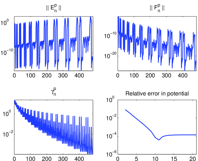
Figure 1: Convergence of the ellipsoidal-harmonic approximation of the Coulomb potential as a function of the degree $n$; the ellipsoid is defined by $a=2$, $b=1.5$, $c=1$, the source charge is at $(0,0,0.5)$, and the field point is $(0,0,2)$.

Our second result demonstrates that the electrostatic solvation free energy of a single charge at the origin recovers the well-known result for the sphere limit, also known as the Born energy, as we model an ellipsoid with semi-axes $a=1+\Delta$, $b=1+\Delta/5$, $c=1+\Delta/10$ (all units in Angstrom), and let $\Delta$ approach zero (Figure 2). These calculations show that the implementations behave correctly for small but finite differences between the ellipsoid semi-axes. Unfortunately, vanishingly small differences pose numerical challenges (note that the ranges for $\mu$ and $\nu$ depend on the differences in the semi-axes). Obtaining the spherical harmonics in the actual limit requires careful analysis Hobson31 ; Dassios03 .

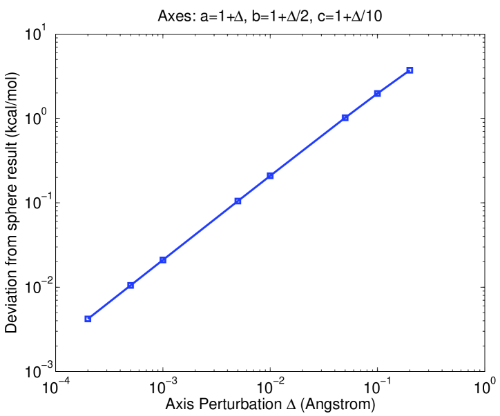
Figure 2: Validating the semi-analytical calculation of electrostatic solvation free energies using the analytical result for a sphere with a central charge (a quantity known as the Born energy). We define $\Delta>0$ and an ellipsoid with semi-axes $a=1+\Delta$, $b=1+\Delta/5$, and $c=1+\Delta/10$. A single $+1e$ charge is situated at the origin, and we have $\epsilon_{1}=4$ and $\epsilon_{2}=80$. As $\Delta\rightarrow 0$, the semi-analytical ellipsoidal results converge to the exact energy for the sphere, which supports the correctness of our implementation.

Finally, using the same dielectric constants as in the previous example, we calculate the electrostatic solvation free energy of a single charge located at $(3,4,5)$ inside a protein-like ellipsoid with semi-axes $a=15$, $b=12$, and $c=10$. For this system, we can validate the implementation numerically using simple BEM calculations, which is also written in MATLAB and included with the ellipsoidal harmonics software. Figure 3 plots the deviation between the semi-analytical result and the numerical BEM results, as a function of the number of boundary elements (flat triangles) used to approximate the ellipsoid surface. We observe the expected linear convergence to the semi-analytical result, which suggests the correctness of our ellipsoidal-harmonic calculation. In the present implementation, more accurate validation is impractical because meshes are generated from within MATLAB using the built-in function ellipsoid, and BEM calculations are performed using dense $O(N^{2})$ algorithms. Fast BEM solvers Lu06 ; Altman09 will be needed for more stringent testing. Also, as Fig. 1 illustrates, more accurate methods need to be found to compute the needed integrals.

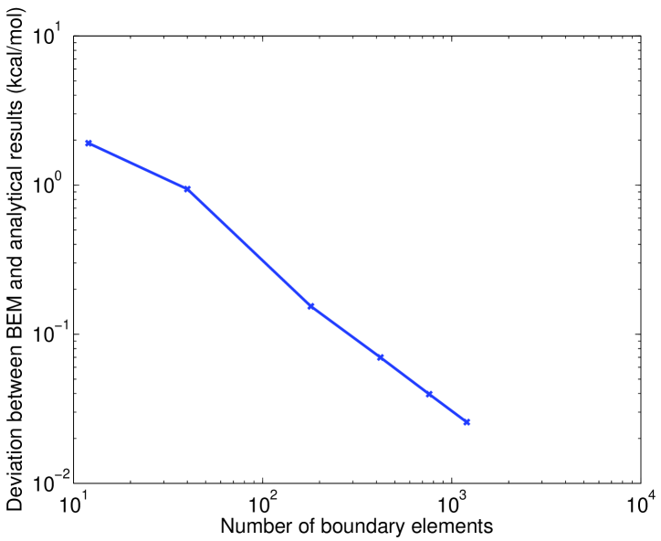
Figure 3: Validating the semi-analytical calculation of electrostatic solvation free energies using numerical simulations based on the boundary-element method (BEM). The ellipsoid has semi-axes $a=15$, $b=12$, and $c=10$, and a single $+1e$ charge is situated inside at $(3,4,5)$; as in Fig. 2, $\epsilon_{1}=4$ and $\epsilon_{2}=80$. The BEM results converge linearly as a function of the number of unknowns (one per panel), which indicates that the semi-analytical method is returning the correct result.

V Discussion

In this paper we have presented two open-source implementations of ellipsoidal harmonics to allow rapid, analytical calculations of many problems of potential theory, including electrostatics, electromagnetics, elasticity, and fluid mechanics. The implementations are written in MATLAB and Python, and released under the Simplified BSD License, and are freely available online LABEL:bitbucket-ellipsoidal. These development efforts stemmed from our interest in improving continuum Poisson-based models of the electrostatic interactions between biological molecules and the surrounding solvent Sharp90_2 ; Honig95 ; Simonson01 . Many important studies have relied on analytically solvable spherical geometries Kirkwood34 , and a variety of state-of-the-art approximate models rely on analyses in spherical harmonics, e.g. Lee02 ; Sigalov05 . We hope that the present implementation of ellipsoidal harmonics, or at least our description of pitfalls we encountered along the way, may provide a starting point for more accurate Generalized-Born models Lee02 ; Sigalov05 or other fast approximations to the Poisson problem Bardhan08_BIBEE ; Bardhan09_bounds ; Bardhan11_bibee .

We do not claim to have covered the entire field of ellipsoidal harmonics, however, or that our implementations are production-level codes with all mathematical subtleties fully addressed. The implementations released with this paper remain under active development, and interested readers are encouraged to contact us with questions, requests, bug reports, and suggestions of all kinds. Currently, the most important area for improvement appears to be in handling coordinate transformations, particularly methods for accurately mapping Cartesian to ellipsoidal coordinates Romain01 , and transformations that seem to need negative $\lambda$ where other publications indicate that non-negative $\lambda$ is adequate. Our results also illustrate the need for more accurate ways to evaluate integrals for the second-kind Lamé functions and the normalization constants.

The present implementation includes the basic algorithms needed to compute the ellipsoidal harmonics, and we have used these primitives to address a fairly simple problem of potential theory (a mixed-dielectric Poisson problem). The primitives can be used for a variety of other problems in potential theory, which are of interest on scales ranging from atoms Perram76 ; Rinaldi82 to entire planets and the solar system Darwin01 ; Romain01 . In addition, recent work by Ritter and colleagues has elucidated the relationship between ellipsoidal harmonics and boundary-integral operators of potential theory for ellipsoidal boundaries (e.g., Ritter95_spectrum ; Ritter98 ). Our approach to approximating biomolecule electrostatic problems using boundary-integral methods Bardhan08_BIBEE ; Bardhan09_bounds ; Bardhan11_bibee should benefit significantly. The most recent analysis employed spherical harmonics and found that accurate approximations could be obtained using parameters that correspond not to spheres but surfaces close to spheres Bardhan11_bibee . We conducted this work because ellipsoids have been used for a number of other molecular electrostatic models Perram76 ; Rinaldi82 ; Rinaldi92 ; Sigalov06 , and thus the boundary-integral analysis of Ritter et al. may allow new approach to approximating the Poisson problem. Also, much of the earlier work employed only the lowest-order modes (which can be expressed in closed form), and did not allow extension to the higher-order ones that must be computed.

In closing: ellipsoidal harmonics have a wide range of applicability, but historically the mechanical details required to use them have been an unfortunate deterrent. Modern computers and numerical algorithms can easily handle these details to enable powerful new modeling tools, and in this work we take a first step towards this goal. It is already clear that computing these functions can motivate more fundamental numerical research, and we hope others will find this subject and its applications equally fascinating. It seems entirely likely that mechanical computation derailed the development of other powerful formalisms in the era before digital computers; perhaps computational science should undertake a journey of re-discovery.

References

- [1] E. W. Hobson. The theory of spherical and ellipsoidal harmonics. Chelsea Pub Co., 1931.
- [2] G. Dassios. Ellipsoidal harmonics: theory and applications. Cambridge University Press, 2012.
- [3] M. G. Knepley and J. P. Bardhan. https://bitbucket.org/knepley/ellipsoidal-potential-theory, 2012.
- [4] K. A. Sharp and B. Honig. Electrostatic interactions in macromolecules: Theory and applications. Annu. Rev. Biophys. Bio., 19:301–332, 1990.
- [5] B. Honig and A. Nicholls. Classical electrostatics in biology and chemistry. Science, 268:1144–1149, 1995.
- [6] Matlab v.6. Mathworks, Inc.
- [7] G. Romain and B. Jean-Pierre. Ellipsoidal harmonic expansions of the gravitational potential: theory and applications. Celestial Mechanics and Dynamical Astronomy, 79:235–275, 2001.
- [8] C. Xue and S. Deng. Three-layer dielectric models for generalized coulomb potential calculation in ellipsoidal geometry. Phys. Rev. E, 83:056709, 2011.
- [9] E. Heine. Handbuch der Kugelfunctionen. Reimer, Berlin, 1878.
- [10] G. H. Darwin. Ellipsoidal harmonic analysis. Proc. Royal Soc. London, 68:248–252, 1901.
- [11] P. M. Morse and H. Feshbach. Methods of Theoretical Physics, Part I and II. McGraw-Hill, New York, NY, USA, 1953.
- [12] P. J. Stiles. Dipolar van der Waals forces between molecules of ellipsoidal shape. Molecular Physics, 38:433–447, 1979.
- [13] J. Yu, C. Jekeli, and M. Zhu. Analytical solutions of the Dirichlet and Neumann boundary-value problems with an ellipsoidal boundary. J. Geodesy, 76:653–667, 2003.
- [14] J. W. Perram and P. J. Stiles. On the application of ellipsoidal harmonics to potential problems in molecular electrostatics and magnetostatics. Proceedings of the Royal Society of London A, 349:125–139, 1976.
- [15] D. Rinaldi. Lamé’s functions and ellipsoidal harmonics for use in chemical physics. Computers and Chemistry, 6:155–160, 1982.
- [16] D. Rinaldi, J.-L. Rivail, and N. Rguini. Fast geometry optimization in self-consistent reaction field computations on solvated molecules. J. Comput. Chem., 13:675–680, 1992.
- [17] G. P. Ford and B. Wang. The optimized ellipsoidal cavity and its application to the self-consistent reaction field calculations of hydration energies of cations and neutral molecules. J. Comput. Chem., 13:229–239, 1992.
- [18] H. Kang and K. Kim. Anisotropic polarization tensors for ellipses and ellipsoids. Journal of Computational Mathematics, 25:157–168, 2007.
- [19] G. Dassios. Second order low-frequency scattering by the soft ellipsoid. SIAM J. Appl. Math., 38:373–381, 1980.
- [20] G. Dassios. The inverse scattering problem for the soft ellipsoid. J. Math. Phys., 28:2858–2862, 1987.
- [21] G. Dassios and F. Kariotou. Magnetoencephalography in ellipsoidal geometry. J. Mathematical Physics, 44:220–241, 2003.
- [22] F. Kariotou. Electroencephalography in ellipsoidal geometry. J. Math. Anal. Appl., 290:324–342, 2004.
- [23] D. E. Woessner. Nuclear spin relaxation in ellipsoids undergoing rotational Brownian motion. J. Chem. Phys., 37:647–655, 1962.
- [24] J. F. Douglas and E. J. Garboczi. Intrinsic viscosity and the polarizability of particles having a wide range of shapes. In Advances in Chemical Physics, volume 91, pages 85–154. 1995.
- [25] G. K. Youngren and A. Acrivos. Rotational friction coefficients for ellipsoids and chemical molecules with the slip boundary condition. J. Chem. Phys., 63:3846–3849, 1975.
- [26] Y. E. Ryabov, C. Geraghty, A. Varshney, and D. Fushman. An efficient computational method for predicting rotational diffusion tensors of globular proteins using an ellipsoid representation. J. Am. Chem. Soc., 128:15432–15444, 2006.
- [27] H. Ammari, H. Kang, and H. Lee. A boundary integral method for computing elastic moment tensors for ellipses and ellipsoids. Journal of Computational Mathematics, 25:2–12, 2007.
- [28] T. Levitina and E. J. Brändas. On the Schrödinger equation in ellipsoidal coordinates. Comput. Phys. Commun., 126:107–113, 2000.
- [29] S. Crozier, L. K. Forbes, and M. Brideson. Ellipsoidal harmonic (lamé) mri shims. IEEE Trans. Superconductivity, 12:1880–1885, 2002.
- [30] J. C.-E. Sten. Ellipsoidal harmonics and their application in electrostatics. J. Electrostatics, 64:647–654, 2006.
- [31] G. Dassios. The Atkinson–Wilcox theorem in ellipsoidal geometry. J. Math. Anal. Appl., 274:828–845, 2002.
- [32] G. Dassios and A. S. Fokas. On two useful identities in the theory of ellipsoidal harmonics. Studies in Applied Mathematics, 123:361–373, 2009.
- [33] G. Dassios, D. Hadjiloizi, and F. Kariotou. The octapolic ellipsoidal term in magnetoencephalography. J. Math. Phys., 50:013508, 2009.
- [34] J. J. Bowman, T. B. A. Senior, and P. L. E. Uslenghi. Electromagnetic and acoustic scattering by simple shapes. North-Holland, Amsterdam, 1969.
- [35] W. E. Byerly. An elementary treatise on Fourier’s series: and spherical, cylindrical, and ellipsoidal harmonics, with applications to problems in mathematical physics. Dover, 2003.
- [36] Ernest William Hobson. 1856-1933. Obit. Not. Fell. R. Soc. 1, 1:236–249, 1934.
- [37] G. Sona. Numerical problems in the computation of ellipsoidal harmonics. J. Geodesy, 70:117–126, 1995.
- [38] H.-J. Dobner and S. Ritter. Attacking a conjecture in mathematical physics by combining methods of computational analysis and scientific computing. Reliable Computing, 3:287–295, 1997.
- [39] S. Ritter. On the computation of Lamé functions, of eigenvalues and eigenfunctions of some potential operators. Z. Angew. Math. Mech., 78:66–72, 1998.
- [40] H.-J. Dobner and S. Ritter. Verified computation of lamé functions with high accuracy. Computing, 60:81–89, 1998.
- [41] W. D. Niven. On ellipsoidal harmonics. Philosophical Transactions of the Royal Society of London A, 182:231–278, 1891.
- [42] J. F. Ahner and R. F. Arenstorf. On the eigenvalues of the electrostatic integral operator. Journal of Mathematical Analysis and Applications, 117:187–197, 1986.
- [43] J. F. Ahner. On the eigenvalues of the electrostatic integral, II. Journal of Mathematical Analysis and Applications, 181:328–334, 1994.
- [44] J. F. Ahner, V. V. Dyakin, and V. Ya. Raevskii. New spectral results for the electrostatic integral operator. Journal of Mathematical Analysis and Applications, 185:391–402, 1994.
- [45] J. F. Ahner, V. V. Dyakin, V. Ya. Raevskii, and St. Ritter. Spectral properties of operators of the theory of harmonic potential. Mathematical Notes, 59(1):3–11, 1996.
- [46] R. G. Langebartel. Some identities for spheroidal harmonics. Astrophysics and Space Science, 175:51–56, 1991.
- [47] Z. Martinec and E. W. Grafarend. Construction of Green’s function to the external Dirichlet boundary-value problem for the Laplace equation on an ellipsoid of revolution. J. Geodesy, 71:562–570, 1997.
- [48] G. Jansen. Transformation properties of spheroidal multipole moments and potentials. J. Phys. A: Math. Gen., 33:1375–1394, 2000.
- [49] J. Ambia-Garrido and B. M. Pettitt. Free energy calculations for DNA near surfaces using an ellipsoidal geometry. Commun. Comput. Phys., 3:1117–1131, 2008.
- [50] A. Di Biasio, L. Ambrosone, and C. Cametti. Dielectric properties of biological cells in the dipolar approximation for the single-shell ellipsoidal model: the effect of localized surface charge distributions at the membrane interface. Phys. Rev. E, 82:041916, 2010.
- [51] Y. Frankel, G. Yossifon, and T. Miloh. Dipolophoresis of dielectric spheroids under asymmetric flows. Physics of Fluids, 24:012004, 2012.
- [52] J. G. Kirkwood. Theory of solutions of molecules containing widely separated charges with special application to zwitterions. J. Chem. Phys., 2:351, 1934.
- [53] B. Z. Lu, X. L. Cheng, J. Huang, and J. A. McCammon. Order N algorithm for computation of electrostatic interactions in biomolecular systems. Proc. Natl. Acad. Sci. USA, 103(51):19314–19319, 2006.
- [54] M. D. Altman, J. P. Bardhan, J. K. White, and B. Tidor. Accurate solution of multi-region continuum electrostatic problems using the linearized Poisson–Boltzmann equation and curved boundary elements. J. Comput. Chem., 30:132–153, 2009.
- [55] K. A. Sharp and B. Honig. Calculating total electrostatic energies with the nonlinear Poisson–Boltzmann equation. J. Phys. Chem., 94(19):7684–7692, 1990.
- [56] T. Simonson. Macromolecular electrostatics: Continuum models and their growing pains. Curr. Opin. Struc. Biol., 11:243–252, 2001.
- [57] M. S. Lee, F. R. Salsbury, and C. L. Brooks III. Novel generalized Born methods. J. Chem. Phys., 116(24):10606–10604, 2002.
- [58] G. Sigalov, P. Scheffel, and A. Onufriev. Incorporating variable dielectric environments into the generalized Born model. J. Chem. Phys., 122:094511, 2005.
- [59] J. P. Bardhan. Interpreting the Coulomb-field approximation for Generalized-Born electrostatics using boundary-integral equation theory. J. Chem. Phys., 129(144105), 2008.
- [60] J. P. Bardhan, M. G. Knepley, and M. Anitescu. Bounding the electrostatic free energies associated with linear continuum models of molecular solvation. J. Chem. Phys., 130:104108, 2009.
- [61] J. P. Bardhan and M. G. Knepley. Mathematical analysis of the boundary-integral based electrostatics estimation approximation for molecular solvation: exact results for spherical inclusions. J. Chem. Phys., 135:124107, 2011.
- [62] S. Ritter. The spectrum of the electrostatic integral operator for an ellipsoid. In R. E. Kleinman, R. Kress, and E. Martensen, editors, Inverse scattering and potential problems in mathematical physics, pages 157–167, Frankfurt/Bern, 1995. Lang.
- [63] G. Sigalov, A. Fenley, and A. Onufriev. Analytical electrostatics for biomolecules: Beyond the generalized Born approximation. J. Chem. Phys., 124(124902), 2006.