Bound–free pair production in ultra–relativistic ion collisions at the LHC collider: Analytic approach to the total and differential cross sections

Abstract

A theoretical investigation of the bound-free electron-positron pair production in relativistic heavy ion collisions is presented. Special attention is paid to the positrons emitted under large angles with respect to the beam direction. The measurement of these positrons in coincidence with the down–charged ions is in principle feasible by LHC experiments. In order to provide reliable estimates for such measurements, we employ the equivalent photon approximation together with the Sauter approach and derive simple analytic expressions for the differential pair–production cross section, which compare favorably to the results of available numerical calculations. Based on the analytic expressions, detailed calculations are performed for collisions of bare Pb⁸²⁺ ions, taking typical experimental conditions of the LHC experiments into account. We find that the expected count rate strongly depends on the experimental parameters and may be significantly enhanced by increasing the positron–detector acceptance cone.
Key words. Bound–free pair production, Relativistic heavy–ion collisions, Virtual photons
PACS 25.75.Dw, 12.20.Ds, 25.75.-q, 03.65.Pm

1 Introduction

Owing to recent advances in heavy–ion accelerators, an increasing interest arises in exploring electromagnetic processes accompanying ion collisions. One of the dominant processes is electron–positron pair production; pertinent cross sections are large. For ultra–relativistic collisions of two bare lead ions (Pb⁸²⁺), for example, the cross section of the creation of a free $e^{+}e^{-}$ pair may reach hundreds of kilobarns BuG75 ; IvS99 ; LeM02 ; LeM09 ; Bau07 . Both free–free as well as bound–free pair production can take place in which the electron is captured by one of the projectiles resulting, thus, in the formation of a hydrogen–like ion,

$$Z_{1}+Z_{2}\to Z_{1}+e^{+}+(Z_{2}+e^{-})\,,$$ (1)

where the bound system is denoted by round brackets. Even though this (bound–free) process is usually orders of magnitude less probable than free–free pair production, its investigation is of great importance not only for a better understanding of the physics of extraordinary strong electromagnetic fields but also for the development and operation of novel collider facilities. In free–free $e^{+}e^{-}$ production, the scattered nuclei lose only a very small fraction of their energy and acquire tiny scattering angles, and thus do not leave the beam. In contrast, if one of the colliding ions captures an electron [cf. Eq. (1)], it changes its charge state and is bent out from the beam. The corresponding cross section is rather large, about $100$ barn, and the reaction (1) is one of the important processes which limit the luminosity of colliders. Besides, the secondary beams of down-charged ions emerging from the collision point hit beam-pipe and deposit a considerable portion of energy at a small spot, which may in turn lead to the quenching of superconducting magnets Bau02 ; JoB05 ; Bru07 ; BrB09 .

Because of its fundamental and practical importance, the bound–free pair production has been in the focus of intense research over the past years. A series of experiments have been performed, for example, at the CERN Super Proton Synchrotron (SPS) to analyze the total cross sections of the process for ultra–relativistic collisions of highly–charged Pb ions with solid–state and gas targets Kra98 ; Kra01 . These experimental findings are currently understood based on theoretical predictions of relativistic Dirac theory BaR96 ; VoN08 . In contrast to the total rates, much less attention has been paid until now to the differential bound-free pair production cross sections. However, the angle–resolved analysis of the positron emission is of definite interest since it allows to probe a parameter range (of the $e^{+}e^{-}$ process) which is otherwise not accessible in total cross section studies. Namely, while the total probabilities arise from a region where the transverse momentum of the produced positron is small, $p_{+\perp}\lesssim m_{e}$, large values of $p_{+\perp}$ may significantly contribute to the angle–differential rates.

An understanding of the differential pair production properties is also significant for the analysis of future experiments at the LHC facility. In these experiments, the down–charged ions can be measured in coincidence with the emitted positrons in order to reduce background events and clearly distinguish the process (1). However, since the central detector is likely to be placed at a rather large angle with respect to the beam direction it will only detect those positrons, whose transverse momenta are much greater than the electron mass, $p_{+\perp}\gg m_{e}$. An estimate of the yield of these positrons is highly desirable for estimating the feasibility of future measurements; the task has not been fully tackled until now to the best of our knowledge.

In this contribution, therefore, we present a theoretical study of bound–free pair production with a special emphasis on the differential cross sections. The exact computations of these cross sections for the ultra–relativistic ion collisions and large positron momenta are very laborious, and we shall develop an approximate method that allows for an analytic treatment. Before discussing the derivation of the analytic expressions, we introduce in Section 2 the notation used in the manuscript and estimate typical values of kinematic parameters corresponding to the LHC experiments. By using these estimates and the equivalent photon approximation (EPA) we express in Sect. 3.1 the differential probabilities of the process (1) in terms of the pair photo–production cross sections. The evaluation of these cross sections within the framework of the Sauter approximation is discussed in Sects. 3.2 and 3.3. The validity of our EPA–Sauter model is tested numerically in Sects. 4.1 and 4.2 where we calculate the total as well as differential pair production rates and compare them with the predictions of an exact relativistic theory. Based on the results of this test, we employ the EPA–Sauter approach in order to estimate the positron yield for ultra–relativistic collisions of bare Pb⁸²⁺ as relevant to the LHC studies. In Sect. 4.2 we focus on two experimental scenarios: In the first scenario, only positrons with very large transverse momenta, $p_{+\perp}\sim 1$ GeV are “seen” by the detectors, while much smaller momenta, $p_{+\perp}\sim 0.05$ GeV, are considered in the second case. We find that the reduction of the (accepted) minimum momentum $p_{+\perp}$ leads to an increase of the positron count rate from just a single event in 67 days to about $10$ events per hour. We conclude with a brief summary in Sect. 5. Through the paper, we use relativistic units with $c=\hbar=1$ and $\alpha\approx 1/137$.

2 Notations and kinematic parameters

Let us first recall basic notations and assumptions used throughout this paper. The initial state of the overall system is given by two bare ions of charges $Z_{1}$ = $Z_{2}$ = $Z$ and masses $M_{1}$=$M_{2}$=$M$, moving towards each other with 4–momenta $P_{1,2}=(E_{1,2},{\vec{P}}_{1,2})$ and corresponding Lorentz–factors $\gamma_{1}$ = $\gamma_{2}$ = $\gamma$. Being defined in the collider frame, these kinematic parameters are convenient for the description of experimental results. However, the theoretical study of atomic processes accompanying ion–ion collisions is most conveniently done in the rest frame of that particular ion which finally becomes hydrogen–like. For definiteness, we shall assume electron to be captured by the “second” nucleus in whose rest frame the “first” nucleus moves with a Lorentz factor $\gamma_{L}=2\gamma^{2}-1$. By adopting $\gamma$ = 1500, which is the typical value for LHC experiments on Pb–Pb ($Z_{1}$ = $Z_{2}$ = 82) collisions, we find $\gamma_{L}=4.5\,\cdot 10^{6}$. This value is used in all numerical estimates below.

Bound–free pair production in energetic ion collisions can be uniquely detected experimentally by measuring the down–charged ion in coincidence with the emitted positron. In the set–up of the typical LHC experimental arrangement, the positron detector is placed at rather large angles with respect to the incident beam direction. Therefore, only positrons with a transverse momentum

$$p_{+\perp}\geq p_{\min}\gg m$$ (2)

can be observed in a particular experiment. In Eq. (2), $m\equiv m_{e}$ is the electron mass and momenta are given in the collider frame. In the same frame, we define the positron’s rapidity:

$$y_{+}=\frac{1}{2}\ln\frac{\varepsilon_{+}+p_{+z}}{\varepsilon_{+}-p_{+z}}\approx-\ln\left[\tan\left(\tfrac{1}{2}\,\theta_{+}\right)\right]\,,$$ (3)

where $\varepsilon_{+}$ and $p_{+z}$ denote the energy and longitudinal (along the beam axis) momentum of the positron and $\theta_{+}$ its emission angle. These quantities are directly related to the transverse momentum, as follows,

$$\varepsilon_{+}\approx\frac{p_{+\perp}}{\sin{\theta_{+}}}\,,\;\;p_{+z}=\frac{p_{+\perp}}{\tan{\theta_{+}}}\,.$$ (4)

Equation (2) immediately implies restrictions both on the rapidity,

$$-y_{\min}\leq y_{+}\leq y_{\min}\,,$$ (5)

as well as on the positron angle,

$$\theta_{\min}\leq\theta_{+}\leq\pi-\theta_{\min}\,,\qquad\theta_{\min}=2\,\arctan\left(\mathrm{e}^{-y_{\min}}\right)\,.$$ (6)

In bound-free pair production, certain limitations are imposed on the electron’s kinematic parameters. As the electron is produced in bound ionic states, its relativistic Lorentz factor and scattering angle match those of the “second” nucleus. Indeed, for ultra–relativistic collisions of heavy high–$Z$ ions, the corresponding scattering angle should be small,

$$\theta_{2}\lesssim\frac{p_{+\perp}}{E_{2}}=\frac{p_{+\perp}}{\gamma\,M}\sim 10^{-5}\,.$$ (7)

Here, all parameters are given in the collider frame. It follows from Eq. (7) and the previous discussion, that the electron’s momentum is almost parallel to the initial direction of propagation of the “second” nucleus, chosen as the $z$–axis:

$$p_{-\perp}\approx 0\,,\qquad p_{-z}\approx\varepsilon_{-}=m\gamma\,.$$ (8)

Using these expressions and Eqs. (2)–(4) for positron emission, we can find the four–momentum $p=(\varepsilon,{\bf p})=(\varepsilon_{+}+\varepsilon_{-},{\bf p}_{+}+{\bf p}_{-})$ and the invariant mass

$$W = \sqrt{p^{2}}\approx\sqrt{2p_{+}p_{-}}=\sqrt{2p_{+\perp}\,m\gamma\,\tan\left(\tfrac{1}{2}\,\theta_{+}\right)}$$ (9)

$$\geq \sqrt{2\,p_{\min}\,m\gamma\,\tan\left(\tfrac{1}{2}\,\theta_{\min}\right)}\,$$

of the final $e^{+}e^{-}$ system.

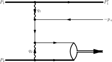
Figure 1: Schematic Feynman diagram for the bound–free pair production in a heavy–nucleus collision. Heavy colliding nuclei are represented by thick lines while thinner lines correspond to light fermions (electron and positron). The trajectory of the produced electron is aligned with that of the second nucleus.

Our theoretical analysis of the bound–free pair production is based on a quantum electrodynamic (QED) approach. In lowest order, the process (1) is described by the diagram in Fig. 1. The exchange of two virtual photons, with four momenta $q_{1,2}=(\omega_{1,2},{\bf q}_{1,2})$, is required to produce the $e^{+}e^{-}$ pair. For the present study, it important to know the virtuality $Q^{2}$ of these photons which measures how far they are off the mass shells. For the first gamma quantum with a 4–momentum $q_{1}=P_{1}-P^{\prime}_{1}$, for example, we write

$$Q^{2}\equiv-q^{2}_{1}\;=\;-\omega_{1}^{2}+q^{2}_{1\perp}+q^{2}_{1z}\;\approx\;q_{1\perp}^{2}+\frac{\omega_{1}^{2}}{\gamma_{1}^{2}}\,,$$ (10)

where we use the fact that

$$\omega_{1}= \;E_{1}-E^{\prime}_{1}\,,\;$$ (11a)

$$q_{1z}\approx \;-E_{1}+\frac{M^{2}}{2E_{1}}+E^{\prime}_{1}-\frac{M^{2}+q^{2}_{1\perp}}{2E^{\prime}_{1}}\,.$$ (11b)

The virtual photons are “emitted” by counter–propagating nuclei, and we finally obtain

$$q_{1z}\approx-\omega_{1}\,,\qquad q_{2z}\approx+\omega_{2}\,.$$ (12)

Together with the four–momentum conservation relations $\omega_{1}+\omega_{2}=\varepsilon$ and $q_{1z}+q_{2z}=p_{z}$ and by employing Eqs. (4) and (8), this allows us to derive the energy of the first virtual photon,

$$\omega_{1} = \frac{1}{2}\left(\varepsilon-p_{z}\right)=\frac{1}{2}\left(\varepsilon_{+}-p_{+z}+\varepsilon_{-}-p_{-z}\right)$$ (13)

$$= \frac{1}{2}\left(\frac{p_{+\perp}}{\sin{\theta_{+}}}-\frac{p_{+\perp}}{\tan{\theta_{+}}}\right)=\frac{1}{2}p_{+\perp}\,\tan\left(\tfrac{1}{2}\,\theta_{+}\right)\,,$$

as a function of the transverse momentum and emission angle of positron. Employing the restrictions given in Eqs. (2) and (6) on these quantities, the minimum allowed value of $\omega_{1}$ can be found,

$$\min\{\omega_{1}\}=\frac{1}{2}\,p_{\min}\,\tan\left(\tfrac{1}{2}\,\theta_{\min}\right)\,.$$ (14)

Before we proceed to the theoretical treatment of the $e^{+}e^{-}$ pair production, let us first compute some typical values for the basic kinematic parameters from above. Assumptions about the magnitude of these values will be required later in order to perform a number of approximations that greatly simplify the calculations of the cross sections. As we have seen already, the ranges of positron as well as virtual photon parameters are crucially depend on the particular experimental set–up. Here, two distinct experimental “scenarios” are considered.

In the first scenario, which relies on a typical LHC–detector acceptance, the transverse momentum and rapidity of the positrons are restricted by the conditions:

$$p_{\min}=1\;\mbox{GeV}\,,\qquad y_{\min}=1\,.$$ (15)

For these parameters, we find

$$\theta_{\min}= \;40^{\circ}\,,$$ (16a)

$$W\geq \;0.75\;\mbox{GeV}\,,$$ (16b)

$$\min\{\omega_{1}\}= \;0.18\;\mbox{GeV}\,,$$ (16c)

for the minimum values of the positron emission angle $\theta_{\min}$, the virtual photon energy $\min\{\omega_{1}\}$ as well as for the $e^{+}e^{-}$ invariant mass $W$, respectively.

In the second scenario, we assume smaller transverse momenta of the positron and a greater rapidity:

$$p_{\min}=0.05\;\mbox{GeV}\,,\qquad y_{\min}=1.5\,,$$ (17)

which results in significantly different parameters:

$$\theta_{\min}= \;25^{\circ}\,,$$ (18a)

$$W\geq \;0.13\;\mbox{GeV},\,,$$ (18b)

$$\min\{\omega_{1}\}= \;5.6\;\mbox{MeV}\,.$$ (18c)

As we see below in Section 4.2, the prospects for a unique detection of bound-free pair production seem much more favorable for the parameters listed in Eq. (18) than for the parameters in scenario (16).

3 Theoretical background

3.1 Equivalent photon approximation

Since its introduction by Fermi Fer24 and further development by von Weizsäcker and Williams, the equivalent photon approximation (EPA) has been successfully applied to the description of a large number of electromagnetic processes induced in collisions of charged particles. Usually, one physically justifies this method based on the observation that the electromagnetic field of a fast moving charge becomes almost transverse, and the electric and magnetic fields both have about equal strengths RaM90 . In the observer (laboratory) frame, therefore, the projectile’s fields can be seen as those of the pulse of a plane, linearly polarized wave. The frequency spectrum of such a pulse is calculated within a semiclassical model and used in order to evaluate collision–induced cross sections EiM95 .

Even though the conventional EPA is found very useful for the theoretical analysis of ion collisions, here we will employ an alternative approach which—in the ultra–relativistic domain—appears to be more transparent and rigorous and allows for a simple estimate of its accuracy. Our approach exploits the EPA as an approximate method for calculating a Feynman diagram for the corresponding process and uses the fact that the virtual photons in the diagram are close to the mass shell—for details, see the review BuG75 . The diagram for bound–free pair production (1) is displayed in Fig. 1, where the two thick lines represent the colliding nuclei and the double–line arrow just refers to the residual hydrogen–like ion. Inspecting this diagram, we may interpret the bound–free pair production as being due to the interaction of the second (lower) nucleus with the virtual (or equivalent) photon with the energy $\omega_{1}$ and virtuality $Q^{2}\equiv-q_{1}^{2}$ emitted by the first nucleus. Thus, the theoretical analysis of the $e^{+}e^{-}$ creation in energetic heavy–ion collisions can be traced back to the virtual process:

$$\gamma^{*}+Z_{2}\to e^{+}+(Z_{2}+e^{-})_{1s}\,,$$ (19)

where the electron is captured into the ground ionic state. The differential cross section d$\sigma_{ZZ}$ of the process (1) can be expressed, therefore, in terms of the cross sections $\sigma^{T}_{\gamma*Z}$ and $\sigma^{S}_{\gamma*Z}$ for the (virtual) pair production (19) as:

$${\mathrm{d}}\sigma_{ZZ}={\mathrm{d}}n_{T}\,{\mathrm{d}}\sigma^{T}_{\gamma*Z}+{\mathrm{d}}n_{S}\,{\mathrm{d}}\sigma^{S}_{\gamma*Z}\,.$$ (20)

In this expression, we denote by ${\mathrm{d}}n_{T}$ and ${\mathrm{d}}n_{S}$ the numbers of the equivalent transverse $T$ and scalar (or longitudinal) $S$ photons and, moreover, neglect the interaction between the emitted positron and the first nucleus.

As seen from Eq. (20), any further evaluation of ${\mathrm{d}}\sigma_{ZZ}$ requires the knowledge of both of the pair photo–production cross sections ${\mathrm{d}}\sigma^{T,S}_{\gamma*Z}$ and infinitesimal numbers ${\mathrm{d}}n_{T,S}$ of equivalent photons. Below we will evaluate these quantities in the rest frame of the second ion, which finally constitutes a hydrogen–like ion. The energy of the equivalent photon, emitted by the first nucleus (cf. Fig. 1), is given in such a frame as:

$$\omega_{L}=\frac{q_{1}P_{2}}{M}\approx 2\gamma\omega_{1}\,.$$ (21)

For the case of an LHC experiment, the minimum value of this energy, $\min\{\omega_{L}\}=2\gamma\min\{\omega_{1}\}$, is huge: it amounts to about $550$ GeV and $17$ GeV for the first (16) and second (18) scenarios, respectively.

In ultra–relativistic nuclear collisions, the main contribution to the pair production cross section (20) is given by a wide range of the photon virtualities (10) ranging from the small minimum value

$$Q^{2}_{\min}=\frac{\omega_{L}^{2}}{\gamma_{L}^{2}}\,,$$ (22)

to some $Q^{2}_{\max}$ which is derived below from the analysis of $\mathrm{d}n_{T,S}$ and the differential cross sections $\mathrm{d}\sigma^{T,S}_{\gamma*Z}$. In such a region, the numbers of equivalent photons are given by (see Appendix D of Ref. BuG75 ):

$$\mathrm{d}n_{S}(\omega_{L},Q^{2}) \sim \mathrm{d}n_{T}(\omega_{L},Q^{2})$$ (23)

$$=\frac{Z_{1}^{2}\alpha}{\pi}\,\frac{\mathrm{d}\omega_{L}}{\omega_{L}}\,\frac{\mathrm{d}Q^{2}}{Q^{2}}\,\left(1-\frac{Q^{2}_{\min}}{Q^{2}}\right)\,F^{2}(Q^{2})\,,$$

where $F(Q^{2})$ is the form factor of the first nucleus.

Integrating Eq. (23) over the interval $[Q^{2}_{\min},Q^{2}_{\max}]$, we find the overall numbers $\mathrm{d}n_{S}(\omega_{L})$ and $\mathrm{d}n_{T}(\omega_{L})$ of the scalar and transverse virtual photons which contribute to the production process (1). For the $dn_{T}(\omega_{L})$ we obtain:

$$\mathrm{d}n_{T}(\omega_{L}) = \frac{Z_{1}^{2}\alpha}{\pi}\,\frac{\mathrm{d}\omega_{L}}{\omega_{L}}$$ (24)

$$\times \int_{Q^{2}_{\min}}^{Q^{2}_{\max}}\frac{\mathrm{d}Q^{2}}{Q^{2}}\,\left(1-\frac{Q^{2}_{\min}}{Q^{2}}\right)\,F^{2}(Q^{2})\,.$$

The evaluation of this integral is discussed in detail in Ref. JeS09 and employs the $Q^{2}$-behavior of the (square of) the nuclear form factor. For example, the function $F^{2}(Q^{2})$ drops quickly when the virtuality of the photon becomes greater than the squared inverse electromagnetic radius of the nucleus, $Q^{2}>1/R^{2}$. Therefore, if $Q^{2}_{\max}\gg 1/R^{2}$, one can simply extend the upper limit of the integration in Eq. (24) to infinity and obtain:

$$\mathrm{d}n_{T}(\omega_{L})=\frac{Z_{1}^{2}\alpha}{\pi}\,\frac{\mathrm{d}\omega_{L}}{\omega_{L}}\,g\left(\omega_{L}\,R/\gamma_{L}\right)\,,$$ (25)

where

$$g(x)=\int_{x^{2}}^{\infty}\frac{{\rm d}y}{y}\,\left(1-\frac{x^{2}}{y}\right)\,F^{2}(y/R^{2})\,$$ (26)

In particular, it was found that for small values of $x=\omega_{L}\,R/\gamma_{L}$, which correspond to the range of parameters considered in the present article, $g(x)$ can be approximated with an accuracy better than 1% as

$$g(x)=\ln\frac{1}{x^{2}}-C_{0}\,,$$ (27)

with $C_{0}=0.163$ for Pb and $C_{0}=0.166$ for Au.

Equations (25) and (27) provide an approximation to the photon number $\mathrm{d}n_{T}(\omega_{L})$ in the regime where $Q^{2}_{\max}\gg 1/R^{2}$. A simple estimate of the $\mathrm{d}n_{T}(\omega_{L})$ can be obtained also for the $Q^{2}_{\max}\ll 1/R^{2}$. In the latter case, the nucleus can be treated as pointlike with the $F(Q^{2})=1$. By inserting this form factor into Eq. (24) we find:

$$\mathrm{d}n_{T}(\omega_{L})=\frac{Z_{1}^{2}\,\alpha}{\pi}\,\frac{\mathrm{d}\omega_{L}}{\omega_{L}}\,\left[\ln\left(\frac{\gamma^{2}_{L}\,Q^{2}_{\max}}{\omega^{2}_{L}}\right)-1\right]\,.$$ (28)

Having clarified the behavior of the photon numbers $\mathrm{d}n_{T,S}$, we now turn to the question of how the cross sections $\mathrm{d}\sigma^{T,S}_{\gamma*Z}(\omega_{L},Q^{2})$, which also enter Eq. (20), depend on the virtuality $Q^{2}$. In order to perform this analysis, we consider pair production in the fields of virtual and real photons. This $\gamma^{*}\gamma\to e^{+}e^{-}$ process is known MeH98 to exhibit very similar behavior as (19), but can be described by simple analytic expressions given in Appendix E of Ref. BuG75 . Namely, while the pair production cross sections $\sigma_{\gamma^{*}\gamma}^{T,S}(W^{2},Q^{2})$ drop drastically at $Q^{2}\gg W^{2}$, the following estimates are valid for smaller values $Q^{2}\ll W^{2}$,

$$\sigma_{\gamma^{*}\gamma}^{S} \lesssim \frac{Q^{2}}{W^{2}}\,\sigma_{\gamma\gamma}\,,$$

$$\sigma_{\gamma^{*}\gamma}^{T} = \sigma_{\gamma\gamma}\,\left[1+{\cal O}\left(\frac{Q^{2}}{W^{2}}\right)\right]\,,$$ (29)

where $\sigma_{\gamma\gamma}=\sigma_{\gamma\gamma}(W^{2})$ describes the $e^{+}e^{-}$ pair production by two real photons.

We are now ready to sum up results of the above analysis and to evaluate the cross sections for the bound-free pair production. For the photon virtualities in the interval $[Q^{2}_{\min},Q^{2}_{\max}]$ (see discussion of Eq. (22)) we can neglect the contribution of the scalar photon and approximate the cross section of the pair production by the transverse photon ${\mathrm{d}}\sigma^{T}_{\gamma*Z}$ by its value ${\mathrm{d}}\sigma^{T}_{\gamma Z}$ on the mass shell (i.e. when $Q^{2}$ = 0). Under these assumptions, Eq. (20) simplifies to

$$\mathrm{d}\sigma^{\rm EPA}_{ZZ}=\mathrm{d}n_{T}(\omega_{L})\,\mathrm{d}\sigma_{\gamma Z}(\omega_{L},p_{+\perp})\,.$$ (30)

The accuracy of such an approximation should be verified for two kinematic regimes. If $W^{2}\gg 1/R^{2}$, which corresponds to the experimental conditions of an LHC detector, the photon’s virtuality is restricted by the nuclear form factor to

$$Q^{2}\lesssim\frac{1}{R^{2}}\ll W^{2}$$ (31)

and we should use the expressions (24)–(27) for the number of the equivalent photons $\mathrm{d}n_{T}(\omega_{L})$. ¿From Eq. (27), we obtain the large Weizsäcker–Williams logarithm $\ell=\ln\left[\gamma^{2}_{L}/(R\omega_{L})^{2}\right]$ that originates from the integral

$$\int_{Q^{2}_{\min}}^{1/R^{2}}\frac{\mathrm{d}Q^{2}}{Q^{2}}\,.$$ (32)

On the other hand, the omitted terms are small,

$$\sim\int_{Q^{2}_{\min}}^{1/R^{2}}\frac{\mathrm{d}Q^{2}}{Q^{2}}\;\frac{Q^{2}}{W^{2}}\sim\frac{1}{R^{2}\,Q^{2}}\ll 1\,,$$ (33)

and do not exhibit logarithmic enhancement. Therefore, the accuracy of the EPA as determined by the relative order of the neglected terms is determined by the factor

$$\eta_{1}\sim\frac{1}{(RW)^{2}\,\ell}<1\,\%\,.$$ (34)

For the total cross section, the main region corresponds to $W^{2}\sim 4m^{2}\ll 1/R^{2}$, and we should use the expression (28) for the number of equivalent photons $\mathrm{d}n_{T}(\omega_{L})$. It contains a large Weizsäcker–Williams logarithm $\sim\ln\gamma^{2}_{L}$. On the other hand, the omitted items are of the order of unity,

$$\sim\int_{Q^{2}_{\min}}^{4m^{2}}\frac{\mathrm{d}Q^{2}}{Q^{2}}\;\frac{Q^{2}}{W^{2}}\sim 1\,,$$ (35)

and again have no logarithmic enhancement. Therefore, the accuracy of EPA in this case is of the order of

$$\eta_{2}\sim\frac{1}{\ln(\gamma^{2}_{L})}\sim 3\,\%\,.$$ (36)

3.2 Bound–free pair photo–production in the Sauter approximation

Finally, as seen from Eq. (30), the computation of $\mathrm{d}\sigma^{\rm EPA}_{ZZ}$ within the EPA can be traced back to the differential cross section of the bound–free pair production following (real rather than virtual) photon impact on a bare nucleus:

$$\gamma+Z\to e^{+}+(Z+e^{-})_{1s}\,.$$ (37)

During the past two decades, this process has been studied in detail with a special emphasis on high–$Z$ ions. The total as well as differential cross sections have been evaluated within a relativistic framework in Refs. AgS97 ; ArS12 . The fully relativistic calculations, based on the partial–wave representation of the Dirac continuum states, were found to provide accurate predictions in the near–threshold region but face well–known problems connected with the slow convergence of the multipole expansions when the photon energy increases. Some approximate methods have to be used, therefore, in order to calculate the cross sections of the process (37) for very high photon energies that correspond to large transfer momenta in ion–ion collisions of the type (1). In the present work, the calculations are based on the Sauter approximation (SA) which was originally derived for the atomic photoeffect by assuming ultra–relativistic electron energies and disregarding terms of relative order $\alpha^{2}Z^{2}$ in an $\alpha Z$–expansion of the transition amplitude Sau31 ; FaM59 ; PrA73 . The general formulas of such an approximation, when applied to the bound–free pair photo-production, are obtained below, while their validity for the high–$Z$ is discussed later in Section 4.2.

The differential cross section for the process (37) can easily be deduced from Sauter’s relativistic formula for the photoeffect or photorecombination, in the notation of Eq. (37) as given, for example, in Eq. (57.8) of Ref. BeL94 upon replacing the electron four–momentum $p$ in the photoeffect with the momentum $(-p_{+})$ of the outgoing positron in the bound-free photo-production (crossing symmetry). More specifically, this implies the following changes:

$$v=\frac{\sqrt{\gamma^{2}-1}}{\gamma}\to-\frac{\sqrt{\gamma_{L}^{2}-1}}{\gamma_{L}}=-v_{+}\,,$$

$$1-v^{2}\to\frac{1}{\gamma_{L}^{2}},\;\;1-\sqrt{1-v^{2}}\to\frac{\gamma_{L}+1}{\gamma_{L}},$$

$$1-v\cos\theta\to 1-v_{+}\cos\vartheta_{+}\,,$$ (38)

where $v_{+}$ and $\vartheta_{+}$ are the velocity and the scattering angle of the positron in the nuclear rest frame, and $\omega_{L}=(\gamma_{L}+1)\,m$ is the photon energy. Performing these substitutions and averaging over the incident photon polarization, we find

$$\frac{\mathrm{d}\sigma^{\rm SA}_{\gamma Z}}{d\Omega_{+}} = \frac{Z^{5}\alpha^{6}}{m^{2}}\frac{v_{+}\sin^{2}{\vartheta_{+}}}{\left(\gamma_{L}+1\right)^{4}\left(1-v_{+}\cos{\vartheta_{+}}\right)^{4}}$$ (39)

$$\times\left[v^{2}_{+}(\gamma_{L}+2)\left(1-v_{+}\cos{\vartheta_{+}}\right)-2\frac{\gamma_{L}-1}{\gamma^{3}_{L}}\right]\,,$$

where, moreover, an additional factor two was included to account for the the different statistical weights of leptons in the initial and final states of the photo-effect and the pair photo-production.

Equation (39), obtained within the Sauter approximation, describes the emission pattern of positrons created in the process (37). Integrating this expression over the positron angles $\vartheta_{+}$, we find the total cross section of pair photo–production,

$$\sigma^{\rm SA}_{\gamma Z}=4\pi\,\frac{Z^{5}\alpha^{6}}{m^{2}}\,G(\gamma_{L})\,,$$ (40)

where the function $G(\gamma_{L})$ is given by:

$$G(x) = \frac{\sqrt{x^{2}-1}}{(x+1)^{4}}\,\Bigg{[}x^{2}+\frac{2}{3}\,x+\frac{4}{3}$$ (41)

$$- \frac{x+2}{\sqrt{x^{2}-1}}\,\ln\left(x+\sqrt{x^{2}-1}\right)\Bigg{]}\,.$$

One may note that this expression coincides with Eq. (52) from Ref. AgS97 upon the replacement $E_{+}=-\gamma_{L}$. In the high–energy limit, $\gamma_{L}\gg 1$, Eq. (40) reads

$$\sigma^{\rm SA}_{\gamma Z}=4\pi\,\frac{Z^{5}\alpha^{6}}{m^{2}\gamma_{L}}\,,$$ (42)

where the dominant contribution is from the first term in square brackets in Eq. (41).

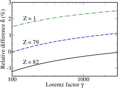
Figure 2: (Color online) The relative difference (55) between rigorous relativistic results and predictions of the scaled EPA–Sauter approximation (54) for the total cross sections of bound–free pair production. Calculations are performed for the energetic collisions between two protons (dash–and–dotted line) as well as bare gold Au⁷⁹⁺ (dashed line) and lead Pb⁸²⁺ (solid line) ions. The EPA–Sauter cross section is given by Eqs. (50) and (3.3) derived using a value of $Q^{2}_{\max}=4m^{2}$.

3.3 Evaluation of total and differential cross sections

In the two previous sections, we have shown how the cross section for the process (19) can be expressed in terms of pair photo–production cross sections and we have evaluated the latter ones within the framework of the Sauter approximation. Now we are ready to conclude this analysis and to derive the final expressions that characterize the positron emission accompanying bound–free pair production in ultra–relativistic collisions between two ions of equal charge:

$$Z_{1}=Z_{2}=Z\,.$$ (43)

For the high–energy and large–momentum transfer regime, where $\gamma_{L}m\gg p_{+\perp}=m\gamma_{L}\vartheta_{+}\gg m$, the differential cross section (39) simplifies to:

$$\mathrm{d}\sigma^{\rm SA}_{\gamma Z}(\omega_{L},p_{+\perp})=16\pi\,\frac{Z^{5}\alpha^{6}}{m^{2}}\;\frac{m}{\omega_{L}}\;\frac{m^{2}\,\mathrm{d}p_{+\perp}}{p_{+\perp}^{3}}\,.$$ (44)

Inserting this expression into Eq. (30), and using the photon number (25), we obtain the cross section

$$\mathrm{d}\sigma^{\rm SA}_{ZZ} = 16\,\frac{\left(Z\alpha\right)^{7}}{m^{2}}\,\frac{m}{\omega_{L}}\,g\left(\frac{\omega_{L}\,R}{\gamma_{L}}\right)\;\frac{\mathrm{d}\omega_{L}}{\omega_{L}}\;\frac{m^{2}\mathrm{d}p_{+\perp}}{\left(p_{+\perp}\right)^{3}}$$

$$= 8\,\frac{\left(Z\alpha\right)^{7}}{m^{2}}\,\frac{m^{3}\,{\rm e}^{y_{+}}}{\gamma\left(p_{+\perp}\right)^{4}}\,g\left(\frac{p_{+\perp}R\,{\rm e}^{-y_{+}}}{2\gamma}\right)\mathrm{d}y_{+}\,\mathrm{d}p_{+\perp}\,,$$

which can be used for an estimate of the positron yield in LHC experiments. The function $g$ is defined in Eqs. (25) and (26). However, since the central detector in such an experiment observes the positrons emitted in a wide range of angles, one has to integrate Eq. (3.3) over the rapidity $y_{+}$ in the interval (5) and over the momentum $p_{+\perp}\geq p_{\min}$ to get the partial cross section $\Delta\sigma^{\rm SA}_{ZZ}$, which is relevant to experimental observation:

$$\Delta\sigma^{\rm SA}_{ZZ}\approx\frac{16}{3}\,\frac{\left(Z\alpha\right)^{7}}{m^{2}}\,\frac{\mathrm{e}^{y_{\min}}}{\gamma}\,\left(\frac{m}{p_{\min}}\right)^{3}\,L\,.$$ (46)

The parameter $L$ is given by

$$L = \left[2\ln\left({\frac{\gamma}{R\,p_{\min}}}\right)+2\,y_{\min}-1.44\right]\,\left(1-{\rm e}^{-2y_{\min}}\right)$$ (47)

$$+4y_{\min}\,\mathrm{e}^{-2y_{\min}}\,.$$

In addition to the partial positron yield (46), we can also employ the Sauter approximation (40) in order to estimate the total bound-free pair production in ultra-relativistic nuclear collisions. We use Eq. (30) together with the number of equivalent photons (28) where we adopt $Q^{2}_{\max}=4m^{2}$, and obtain (upon integration over the photon energy):

$$\sigma^{\rm EPA}_{ZZ} = \int_{2m}^{\infty}\mathrm{d}n_{T}(\omega_{L})\,\sigma^{\rm SA}_{\gamma Z}(\omega_{L})$$ (48)

$$= 4\,\frac{(Z\alpha)^{7}}{m^{2}}\,\left\{a\left[\ln(4\gamma^{2}_{L})-1\right]-b\right\}\,,$$

where the parameters $a$ and $b$ can be evaluated analytically,

$$a = \int_{1}^{\infty}G(x)\,\frac{{\rm d}x}{x+1}=\frac{137}{630}=0.2175\,,$$

$$b = \int_{1}^{\infty}G(x)\,\ln{(x+1)}\,\frac{{\rm d}x}{x+1}$$ (49)

$$= \frac{57\,707-19\,180\,\ln 2}{88\,200}=0.5035\,.$$

By taking into account that $\gamma_{L}$ is defined in terms of the nuclear Lorentz factors as $\gamma_{L}=2\gamma^{2}-1$ we obtain from Eq. (48) the well–known scaling law:

$$\sigma^{\rm EPA}_{ZZ}=A\ln\gamma-B\,,$$ (50)

where $A$ and $B$ are predicted to be independent of $\gamma$ BaR91 ; BaR93 ; KrV98 . The values of these two parameters, as estimated within the equivalent photon approximation, depend on the particular choice of the maximal photon virtuality $Q^{2}_{\max}$. For example, based on our estimate $Q^{2}_{\max}=4m^{2}$ which was recommended in Ref. MeH98 , we find:

$$A = 16\frac{(Z\alpha)^{7}}{m^{2}}\,a=3.479\,\frac{(Z\alpha)^{7}}{m^{2}}=5.72\,Z^{7}\;\mbox{pb}\,,$$

$$B = 8\frac{(Z\alpha)^{7}}{m^{2}}\,\left[b-a(\ln 4-0.5)\right]=2.49\,\frac{(Z\alpha)^{7}}{m^{2}}$$ (51)

$$= 4.09\,Z^{7}\;\mbox{pb}\,,$$

which are in the picobarn range (pb). By contrast, the different value $Q^{2}_{\max}=1.26\,m^{2}$ adopted in Ref. Ast07 yields

$$A=3.479\,\frac{(Z\alpha)^{7}}{m^{2}}\,,\qquad B=3.49\,\frac{(Z\alpha)^{7}}{m^{2}}\,.$$ (52)

As seen from Eqs. (3.3) and (52), while the parameter $A$ is not sensitive to the change of $Q^{2}_{\max}$, the parameter $B$ varies by about 40 % which is quite remarkable but still within the accuracy of the EPA.

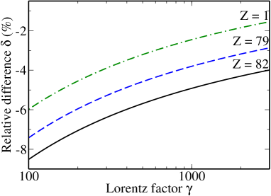
Figure 3: (Color online) The same as in Fig. 2, but the EPA–Sauter cross section is given by Eqs. (50) and (52) employing a value of $Q^{2}_{\max}=1.26\,m^{2}$.

4 Results and discussion

4.1 Total cross sections

Although the main goal of the present paper is to provide reliable estimates for the positron yield as might be measured by the central detector of an LHC experiment, we start calculations with the total pair production cross sections. Their analysis, performed for different nuclear charges and various collision energies, can help to better define the range of validity for our EPA–Sauter model. In order to start with such an analysis, let us recall that the high–energy limit of the Sauter photo–production cross section (42) is known to differ from the exact results by some factor:

$$\sigma^{\rm exact}_{\gamma Z}=f(Z)\,\sigma^{\rm SA}_{\gamma Z}\,,\qquad\omega_{L}\to\infty\,,$$ (53)

where $f(Z)$ is a decreasing function of the nuclear charge Pra60 ; MiS93 ; AsH94 . Values for $f(Z)$ are obtained in Ref. AgS97 based on rigorous relativistic calculations. For example, for the $e^{+}e^{-}$ production in which the electron is captured into the ground state of an initially bare ion, these calculations predict $f(Z)=0.971,0.222,0.216$ and $0.196$ for $Z=1,79,82$ and $92$, respectively.

In the following we shall apply the factor $f(Z)$ to improve also the accuracy of approximations (46) and (50) that describe the bound–free pair production in heavy ion collisions. For the total cross section of this process, for example, we make the replacement:

$$\sigma^{\rm EPA}_{ZZ}\to f(Z)\cdot\sigma^{\rm EPA}_{ZZ}=f(Z)\,\left(A\ln\gamma-B\right)\,.$$ (54)

As seen from Fig. 2, where the relative difference

$$\delta=\frac{f(Z)\cdot\sigma^{\rm EPA}_{ZZ}-\sigma^{\rm exact}_{ZZ}}{\sigma^{\rm exact}_{ZZ}}$$ (55)

between the scaled EPA–Sauter cross section and exact results $\sigma^{\rm exact}_{ZZ}$ from Ref. MeH01 is displayed, such a replacement leads to a very good agreement between the predictions of the two theories (EPA–Sauter and rigorous relativistic calculations MeH01 ). In particular, for energetic collisions of two gold (dashed line) and led (solid line) ions the relative difference $\delta$ does not exceed 1.5 % for Lorentz parameters in the range 100 $\leq\gamma\leq$ 3000. It is worth mentioning that a slightly worse performance of the EPA–Sauter approximation can be observed if in place of the photon virtuality $Q^{2}_{\max}=4m^{2}$, used to derive values (3.3), the $Q^{2}_{\max}=1.26\,m^{2}$ from Ref. Ast07 is adopted. For the latter case, the relative difference between the exact and EPA predictions may reach $6\div 12\,\%$ in the low–energy domain (see Fig. 3).

4.2 Differential cross sections

Having briefly discussed computations of the total bound-free pair production cross sections, we now estimate the differential pair production probabilities. In order to assess the reliability of these predictions, let us first verify the accuracy of Eq. (44) for $\mathrm{d}\sigma^{\rm SA}_{\gamma Z}$, and Eq. (3.3) for $\mathrm{d}\sigma^{\rm SA}_{ZZ}$. These formulates are based on the Sauter approximation (39) for the $e^{+}e^{-}$ photo–production. Since this approximation is correct only in the leading order of $\alpha Z$, its validity in the high–$Z$ domain has to be examined. To this end, in Fig. 4, we display the differential cross sections $\mathrm{d}\sigma^{\rm exact}_{\gamma Z}/\mathrm{d}\Omega_{+}$ of the process (37) for the photon collision with bare led ions Pb⁸²⁺ and emitted positron energies $m\gamma_{L}$ with $\gamma_{L}$= 5, 10, 15 and 25. Results of rigorous relativistic theory, which employs the standard partial-wave decomposition of continuum Dirac wavefunctions ArS12 , are compared with scaled predictions of Eq. (39), obtained as follows,

$$\frac{\mathrm{d}\sigma^{\rm SA}_{\gamma Z}}{\mathrm{d}\Omega_{+}}\to f(Z)\cdot\frac{\mathrm{d}\sigma^{\rm SA}_{\gamma Z}}{\mathrm{d}\Omega_{+}}\,,$$ (56)

where $f(Z)$ is the same factor as employed in Eq. (53). One may note that the previously observed, good performance of this scaling for the total rates (the main contribution to which comes from forward positron emission, $\vartheta_{+}\lesssim 1/\gamma_{L}$), does not automatically guarantee accurate results for the differential cross sections, especially in the region of larger emission angles. Fortunately, the results presented in Fig. 4 clearly indicate the validity of this scaling. Namely, even though the (scaled) Sauter approximation can significantly underestimate exact results for forward as well as backward positron emission, the range of angles, over which the two theories differ significantly, shrinks with increasing positron energy. For example, while for $\gamma_{L}=5$, the Sauter approximation reproduces the exact results with the accuracy of about 5 % only for the angles $50^{\circ}<\vartheta_{+}<60^{\circ}$, this interval increases to $2^{\circ}<\vartheta_{+}<120^{\circ}$ for $\gamma_{L}=25$. These findings justify the application of the Sauter approximation together with the scaling (44) for the analysis of the pair production in ultra–relativistic heavy ion collisions at an LHC experiment in which large positron transverse momenta, $p_{+\perp}$, will be monitored.

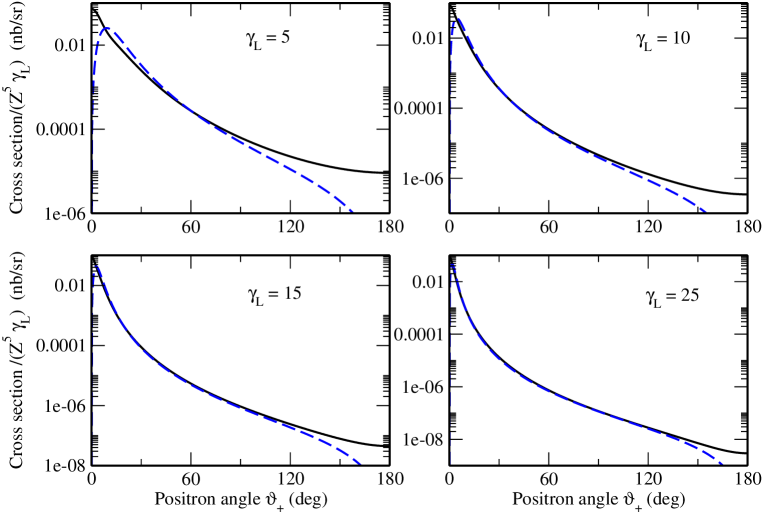
Figure 4: (Color online) The differential cross section $(Z^{5}\,\gamma_{L})^{-1}\,\mathrm{d}\sigma_{\gamma Z}/\mathrm{d}\Omega_{+}$ (in nanobarn/steradian) of the pair production in the collision of photon with bare lead Pb⁸²⁺ ion accompanied by the electron capture into the ground ionic state. Results of the rigorous relativistic calculations (solid line) are compared to the predictions of the scaled Sauter approximation (dashed line). Calculations have been performed in the nucleus rest frame and four positron energies $m\gamma_{L}$ with $\gamma_{L}=5,10,15$ and $25$.

Besides the direct numerical “proof”, yet another confirmation of the scaling conjecture (56) was recently received. Namely, the asymptotic behavior of the pair–production differential cross section in the region $m^{2}\ll p^{2}_{+\perp}\ll 2m\omega_{L}$ was derived for arbitrary $Z\alpha$ in Ref. Mil12 . This asymptotic reads as

$$\mathrm{d}\sigma^{\rm exact}_{\gamma Z}(\omega_{L},p_{+\perp})=f^{\rm asymp}(Z)\,16\pi\frac{Z^{5}\alpha^{6}}{m^{2}}\;\frac{m}{\omega_{L}}\;\frac{m^{2}\,\mathrm{d}p_{+\perp}}{p_{+\perp}^{3}}\,,$$

$$f^{\rm asymp}(Z)=\frac{2\,(2\eta)^{2\tilde{\gamma}-2}}{\Gamma(2\tilde{\gamma}+1)}\,\,|\Gamma(\tilde{\gamma}-{\rm i}\eta)|^{3}\,{\rm e}^{-2\eta\arccos{\eta}}\,,$$ (57)

where $\eta=Z\alpha$ and $\tilde{\gamma}=\sqrt{1-\eta^{2}}$. One obtains from this expression $f^{\rm asymp}(Z)$ = 0.297, 0.287 and 0.257 for $Z$ = 79, 82 and 92. Therefore, our assumptions about scaled factor $f(Z)$ are by about 25 % smaller then the corresponding factor $f^{\rm asymp}(Z)$ for the same values of $Z$. We note that such a discrepancy is comparable to the (expected) experimental error and the overall uncertainty of our model that arises not only from the use of the Sauter and EPA approximations but also from neglecting the electron capture into excited ionic states, an effect which will be briefly addressed later.

Based on the accuracy analysis of the scaled Sauter approximation (44) for $\mathrm{d}\sigma^{\rm SA}_{\gamma Z}$ and (56) for $\mathrm{d}\sigma^{\rm SA}_{ZZ}$, we are now in the position to compute the positron yield. This yield is defined by the partial cross section given in Eq. (46), which has to be scaled properly,

$$\Delta\sigma^{\rm SA}_{ZZ}\to 2\,f(Z)\,\Delta\sigma^{\rm SA}_{ZZ}\,.$$ (58)

The factor two accounts for the fact that the electron can be captured by either of two nuclei. Assuming a maximum luminosity $\mathcal{L}=10^{27}\,{\rm s}^{-1}\,{\rm cm}^{-2}$ which can be reached in Pb–Pb collision experiments at CERN, and using the corresponding sets of kinematic parameters $\{y_{\rm min},p_{\rm min}\}$ (see Sect. 2), we finally obtain from Eqs. (46) and (58) that (i) only one event per 67 days is likely to be observed for the high–transverse–momentum scenario (15), whereas (ii) about 16 counts per hour are within the acceptance range of the detector within the scenario (17).

One may note that these estimates were obtained based on the assumption that the electron is captured into the ground ionic states. The $e^{+}e^{-}$ pair production accompanied by the formation of excited hydrogen–like ions may slightly increase these predictions. However, Refs. AgS97 ; LeM04 indicate that the effect of the excited state electron recombination shall not exceed $20\div 25\,\%$.

5 Summary and outlook

In conclusion, we investigate bound–free pair production in ultra–relativistic heavy ion collisions. Special emphasis in our study is placed on the emission of positrons with large transverse momenta which can be observed at the LHC collider. In order to estimate the yield of such positrons, an approximate method, based on the equivalent photon approximation and the Sauter theory, has been laid out. Within the EPA–Sauter approach, we derive a simple analytical expression for the differential cross section of the pair production process (1). Based on this expression, calculations have been performed for the collisions between two bare lead ions Pb⁸²⁺ moving towards each other with the Lorentz factor $\gamma$ = 1500. At this energy, typical for the LHC, we consider two scenarios that correspond to different detectors set-ups. While for the first scenario (15) the number of events is too small to be measured, the second scenario (17) looks rather promising. Our conceptually simple approach allows us to incorporate the detector set–up into the final formulas for the partial cross sections relevant to experimental observation at the LHC. Essentially, we conclude that in the first scenario (15), bound-free pair production takes place but most of the positrons escape the detector; they are not sufficiently deflected out of the beam line to be within the acceptance range of the LHC detectors.

In the present work we have restricted our theoretical analysis to a single $e^{+}e^{-}$ production. In the ultra–relativistic regime, however, the ion–ion collisions may result in the creation of a few electron–positron or even muon–antimuon pairs. Such a multiple–pair (and heavier lepton) production now attracts considerable attention as a tool for exploring the quantum electrodynamics in extremely strong electromagnetic fields AlH97 ; Bal09 . In heavy ion colliders, these processes again can be explored by measuring the emitted positrons and residual few–electron ions in coincidence. Theoretical predictions, required for preparing and analyzing such coincidence experiments, may be naturally obtained within the framework of the EPA–Sauter theory. Investigations along this line are currently underway and will be presented in a future paper.

References

- (1) V. M. Budnev, I. F. Ginzburg, G. V. Meledin, V. G. Serbo, Phys. Reports 15, 181 (1975)
- (2) D. Yu. Ivanov, A. Schiller, V. G. Serbo, Phys. Lett. B 454, 155 (1999)
- (3) R. N. Lee, A. I. Milstein, V. G. Serbo, Phys. Rev. A 65, 022102 (2002)
- (4) R. N. Lee, A. I. Milstein, Zh. Exp. Teor. Fiz., 136, 1121 (2009), [JETP 109, 968 (2009)]
- (5) G. Baur et al., Phys. Rep. 453, 1 (2007)
- (6) G. Baur et al., Phys. Rep. 364, 359 (2002)
- (7) J. M. Jowett, R. Bruce, S. Gilardoni, Proc. of the Particle Accelerator Conf. 2005, Knoxville p. 1306 (2005).
- (8) R. Bruce et al., Phys. Rev. Lett. 99, 144801 (2007)
- (9) R. Bruce, D. Bocian, S. Gilardoni, J. M. Jowett, Phys. Rev. ST Accel. Beams 12, 071002 (2009)
- (10) H. F. Krause et al., Phys. Rev. Lett. 80, 1190 (1998)
- (11) H. F. Krause et al., Phys. Rev. A 63, 032711 (2001)
- (12) A. J. Baltz, M. J. Rhoades–Brown, J. Weneser, Phys. Rev. E 54, 4233 (1996)
- (13) A. B. Voitkiv, B. Najjari, A. Surzhykov, J. Phys. B: At. Mol. Opt. Phys. 41, 111001 (2008)
- (14) E. Fermi, Z. Phys. 29, 315 (1924)
- (15) J. Rau, B. Muller, W. Greiner, G. Soff, J. Phys. G: Nucl. Part. Phys. 16, 211 (1990)
- (16) J. Eichler, W. E. Meyerhof, Relativistic Atomic Collisions, pp. 47–59, Academic Press, San Diego (1995).
- (17) U. D. Jentschura, V. G. Serbo, Eur. Phys. J. C 64, 309 (2009)
- (18) H. Meier, Z. Halabuka, K. Hencken, D. Trautmann, G. Baur, Eur. Phys. J. C 5, 287 (1998)
- (19) C. K. Agger, A. H. Sörensen, Phys. Rev. A 55, 402 (1997)
- (20) A. N. Artemyev, A. Surzhykov, in preparation
- (21) F. Sauter, Ann. Physik 9, 217 (1931)
- (22) U. Fano, K. W. McVoy, J. R. Albers, Phys. Rev. 116, 1147 (1959)
- (23) R. H. Pratt, A. Ron, H. K. Tseng, Rev. Mod. Phys. 45, 273 (1973)
- (24) V. B. Berestetskii, E. M. Lifshitz, L. P. Pitaevskii, Quantum Electrodynamics, Pergamon Press (1994).
- (25) A. J. Baltz, M. J. Rhoades–Brown, J. Weneser, Phys. Rev. A 44, 5668 (1991)
- (26) A. J. Baltz, M. J. Rhoades–Brown, J. Weneser, Phys. Rev. A 50, 4842 (1993)
- (27) H. F. Krause et al., Phys. Rev. Lett. 80, 1190 (1998).
- (28) A. Aste, Eur. Phys. Lett. 81, 61001 (2007)
- (29) R. H. Pratt, Phys. Rev. 117, 1017 (1960)
- (30) A. I. Milstein, V. M. Strakhovenko, Zh. Eksp. Teor. Fiz. 103, 1584 (1993) [JETP 76, 775 (1993)]
- (31) A. Aste, K. Hencken, D. Trautmann, G. Baur, Phys. Rev. A 50, 3980 (1994)
- (32) H. Meier, Z. Halabuka, K. Hencken, D. Trautmann, G. Baur, Phys. Rev. A 63, 032713 (2001)
- (33) R. N. Lee, A. I. Milstein, V. M. Strakhovenko, Phys. Rev. A 69, 022708 (2004)
- (34) A. Alscher, K. Hencken, D. Trautmann, G. Baur, Phys. Rev. A 55, 396 (1997)
- (35) A. J. Baltz, Phys. Rev. C 80, 034901 (2009)
- (36) A. Di Piazza, A.I. Milstein, arXive: 1203.2137 [physics.atom-ph]