Magnetized dark energy and the late time acceleration

Abstract

In the present work we have searched the existence of the late time acceleration of the Universe. The matter source that is responsible for the late time acceleration of the Universe consists of cosmic fluid with the equation of state parameter $\omega=p/\rho$ and uniform magnetic field of energy density $\rho_{B}$. The study is done here under the framework of spatially homogeneous and anisotropic locally rotationally symmetric (LRS) Bianchi-I cosmological model in the presence of magnetized dark energy. To get the deterministic model of the Universe, we assume that the shear scalar $(\sigma)$ in the model is proportional to expansion scalar $(\theta)$. This condition leads to $A=B^{n}$, where $A$ and $B$ are metric functions and $n$ is a positive constant giving the proportionality condition between shear and expansion scalar. It has been found that the isotropic distribution of magnetized dark energy leads to the present accelerated expansion of the Universe and the derived model is in good agreement with the recent astrophysical observations. The physical behavior of the Universe has been discussed in details.

1 Introduction

The cosmological observations from type Ia supernovae Riess1998 ; Perlmutter1999 , cosmic microwave background (CMB) and clusters of galaxies Pope2004 etc, all suggest that the expansion of the present Universe is speeding up rather than slowing down. This at once indicates that the baryon matter component is about $4\%$ of the total energy density and about $96\%$ of the energy density in the Universe is invisible which opposes the self attraction of matter and causes the observed expansion of the Universe to accelerate. This acceleration is characterized by the negative pressure and the positive energy density and hence violates the strong energy condition. This violation gives a reverse gravitational effect. Due to this effect, the Universe gets a jerk and the transition from the earlier deceleration phase to the recent acceleration phase takes place Caldwell2006 .

In physical cosmology and astrophysics, the simplest candidate for the dark energy (DE) is the cosmological constant $(\Lambda)$ Carroll2001 ; Peebles2003 . However, it needs to be extremely fine-tuned to satisfy the current value of the DE density, which is a serious problem Overduin1998 . Alternatively, to explain the decay of the density, the different forms of dynamically changing DE with an effective equation of state (EoS), $\omega=p/\rho<-1/3$, were proposed instead of the constant vacuum energy density. There are several other possible forms of DE such as quintessence $(\omega>-1)$ Steinhardt1999 , phantom $(\omega<-1)$ Caldwell2002 etc. It is observed that current cosmological data from SN Ia (Supernovae Legacy Survey, Gold sample of Hubble Space Telescope) Riess2004 ; Astier2006 , CMBR (WMAP, BOOMERANG) Eisentein2005 ; MacTavish2006 and large scale structure (Sloan Digital Sky Survey) Komatsu2009 do not support possibility of $\omega<<-1$. However, time-dependent DE characterized by $\omega=-1$ and crossing the phantom divide line even now is a favorable candidate. The limit obtained from observational results coming from CMBR anisotropy and galaxy clustering is $-1.44<\omega<-0.92$ with $68\%$ confidence level Komatsu2009 ; Hinshaw2009 .

Under the above circumstances, it is observed that in recent years Bianchi universes have been gaining an increasing interest and tremendous impetus of observational cosmology. In connection to the WMAP data Hinshaw2009 ; Hinshaw2003 ; Jaffe2005 it is now revealed that the standard cosmological model requires a positive and dynamic cosmological parameter that resembles the Bianchi morphology Jaffe2006a ; Jaffe2006b ; Campanelli2006 ; Campanelli2007 . According to this, the Universe should achieve the following features: (i) a slightly anisotropic special geometry in spite of the inflation, and (ii) a nontrivial isotropization history of Universe due to the presence of an anisotropic energy source. The anomalies found in the cosmic microwave background (CMB) and large scale structure observations stimulated a growing interest in anisotropic cosmological model of Universe. Here we confine ourselves to model LRS Bianchi-I whose spatial sections are flat but the expansion or contraction rate are direction dependent. For studying the possible effects of anisotropy in the early Universe based on the present day observations many researchers Huang1990 ; Chimento1997 ; Lima1996 ; Lima1994 ; Pradhan2004 ; Saha2006a ; Saha2006b have investigated Bianchi type-I models from different point of view. We notice that, in connection to anisotropic equation of state for dark energy, several works are now available in the literature Richard2009 ; Campanelli2010 ; Stephen2011 . Some Authors Akarsu2010 ; Kumar2011 ; Amirhashchi2011 ; Yadav2011a ; Yadav2011b ; Yadav2011c ; Yadav2011d have studied anisotropic DE models even with constant deceleration parameter (DP).

We would like to further mention that unlike the FRW model this Bianchi-I type model describes a different kind of Universe in which the scale factor is not restricted to be the same in each direction. In the present work, following King and Coles King2007 , we assume a large scale homogeneous magnetic field which is responsible for the anisotropy in the flat Universe. It is expected that such a magnetic field will impose a single preferred direction in space. Therefore, under the influence of this directional magnetic field along the field lines the anisotropy of the spacetime will be axisymmetric. However, it is argued by King and Coles King2007 that the observed level of isotropy in the CMB places tight constraints upon the strength of any Hubble scale magnetic field. The upper limit on such a field is found to be of the order of $10^{-9}$ Gauss Barrow1997 . King and Coles King2007 also state that these and other similar limits quote the adiabatically expanded, present-day equivalent very weak value of the field strength which equate to a much stronger field at very early times.

It is a obvious question then - does the above size of the magnetic field satisfy all observational constraints at the different scales? An extensive field survey provides that (i) the lowest measured intergalactic fields and close to the observational upper limits via Faraday rotation measurements Kim1991 ; Perley1991 ; Kronberg1994 , may well be of cosmological origin; (ii) a similar protogalactic field strength is inferred from the detection of fields of order $10^{-6}$ Gauss in high redshift galaxies Kronberg1992 and in damped Lyman alpha clouds Wolfe1992 , (iii) primordial nucleosynthesis constraints only limit the equivalent current epoch field to be less than about $10^{-7}$ Gauss Grasso1995 , a value that is only slightly stronger than the dynamical constraint at nucleosynthesis Thorne1967 ; Doroshkevich1967 ; Jacobs1969 .

Regarding the impact of magnetic field it is argued that in the early times, the magnetic field had the significant role on the dynamics of the Universe depending on the direction of the field lines Maden1989 ; King2007 . Several authors have used Bianchi models to investigate the influence of the magnetic field on the evolution of the Universe. It is worth noting that there has been some work on magnetic fields in Bianchi I models in the past Jacobs1969 ; Milaneschi1985 ; LeBlanc1997 ; Tsagas2000 . Milaneschi and Fabbri Milaneschi1985 studied the anisotropy and polarization of CMB radiation where as, Jacobs Jacobs1969 explored the effect of a uniform primordial magnetic field. Both the investigating groups used Bianchi-I model of the Universe. Jacobs Jacobs1969 argued that in the early stages of the evolution of the Universe, the magnetic field produced large expansion anisotropies during the radiation-dominated phase whereas it has negligible effect during the dust-dominated phase.

In the relatively recent works, it is seen that King and Coles King2007 have used the magnetized perfect fluid energy-momentum tensor to discuss the effects of magnetic field on the evolution of Universe. Sharif and Zubair Sharif2010 have studied dynamics of Bianchi-I universe with magnetized field of anisotropic dark energy.

In the present work, however, we present a magnetized dark energy model with time varying DP in LRS Bianchi-I spacetime. The investigation is organized as follows: The metric and field equations are presented in section 2. Section 3 deals with the exact solutions of field equations and physical behavior of the model. The comparison between distance modulus $(\mu)$ of derived model and observational $\mu(z)$ is presented in section 4 respectively. Finally the results are discussed in section 5.

2 The Metric and Field Equations

We consider the LRS Bianchi type I metric of the form

$$ds^{2}=-dt^{2}+A(t)^{2}dx^{2}+B(t)^{2}\left(dy^{2}+dz^{2}\right).$$ (1)

where, A and B are functions of $t$ only. In the limit where $A(t)=B(t)$, the metric equation (1) reduces to flat FRW metric. Here the geometry of space-time (1) is represented by two equivalent transverse directions $y$ and $z$ and one different longitudinal direction $x$, along which the magnetic field is oriented i. e. $A=A_{x}$ only.

The Einstein’s field equations, in the units $8\pi G=c=1$, read as

$$R^{i}_{j}-\frac{1}{2}g^{i}_{j}R=-T^{i}_{j},$$ (2)

where $T^{i}_{j}$ is the energy momentum tensor cosmic fluid and it is given by

$$T^{i}_{j}=diag[\rho-\rho_{B},-\omega\rho+\rho_{B};,-\omega\rho-\rho_{B},-\omega\rho-\rho_{B}],$$ (3)

where $\rho$ is the energy density of cosmic fluid, $\rho_{B}$ is the energy density of magnetic field, $\omega=p/\rho$ is the EoS parameter of cosmic fluid and $p$ is the pressure of the cosmic fluid. It is important to note here that the EoS parameter $(\omega)$ is not necessarily constant Carroll2003 .

It is to note that the energy momentum for cosmic fluid given in Eq. (3) is a system of perfect fluid and magnetic field in a comoving coordinates i.e. $T_{i}^{j}=T_{i}^{j}(PF)+E_{i}^{j}$. Here, $E_{i}^{j}$ is the electromagnetic field. We choose the magnetic field along $x$-direction. In our model, the electromagnetic field tensor $F^{ij}$ has only one non-vanishing component, viz., $F_{yz}=$ constant. Therefore, for the electromagnetic field tensor $E^{i}_{j}$, one gets the following non-trivial components, $E_{t}^{t}=E_{x}^{x}=-E_{y}^{y}=-E_{z}^{z}=\rho_{B}$.

Therefore, the Einstein’s field equations (2) for the line-element (1) reduce to the following system of equations

$$2\frac{\ddot{B}}{B}+\frac{\dot{B}^{2}}{B^{2}}=-\omega\rho+\rho_{B}\;,$$ (4)

$$\frac{\ddot{A}}{A}+\frac{\ddot{B}}{B}+\frac{\dot{A}\dot{B}}{AB}=-\omega\rho-\rho_{B}\;,$$ (5)

$$\frac{\dot{B}^{2}}{B^{2}}+2\frac{\dot{A}\dot{B}}{AB}=\rho+\rho_{B}.$$ (6)

Here, and in what follows, over-dots indicates differentiation with respect to $t$. The energy conservation equations $T^{i}_{j;i}=0$, related to the two equations for cosmic fluid and magnetic field King2007 , are as follows

$$\dot{\rho}+3(1+\omega)\rho H=0,$$ (7)

$$\rho_{B}=\frac{\beta}{B^{4}}.$$ (8)

Here $\beta$ is positive constant and $H$ is the mean Hubble parameter, which for LRS Bianchi-I space-time can be defined as

$$H=\frac{\dot{a}}{a}=\frac{1}{3}\left(\frac{\dot{A}}{A}+2\frac{\dot{B}}{B}\right),$$ (9)

with $a$ being the average scale factor of LRS Bianchi type-I model and can be expressed as

$$a=(AB^{2})^{\frac{1}{3}}.$$ (10)

It seems that any radiation field with the evolution law expressed in Eq. (8) would work. However, one may raise a tricky question that why does this field only scale with the scale factor $B$? It can be verified that if one writes the conservation equation for cosmic fluid and the magnetic field separately, then one can get Eq. (8) which contains only scale factor $B$.

The spatial volume (V) is given by

$$V=a^{3}=AB^{2}.$$ (11)

The expansion scalar ($\theta$), the shear scalar ($\sigma$) and the mean anisotropy parameter ($A_{m}$) are defined as

$$\theta=3H=\frac{\dot{A}}{A}+2\frac{\dot{B}}{B},$$ (12)

$$\sigma^{2}=\frac{1}{2}\left(\sum_{i=1}^{3}H_{i}^{2}-\frac{1}{3}\theta^{2}\right),$$ (13)

$$A_{m}=\frac{1}{3}\sum_{i=1}^{3}\left(\frac{H_{i}-H}{H}\right)^{2},$$ (14)

where $H_{i}(i=1,2,3)$ represent the directional Hubble parameters in the direction of $x$, $y$ and $z$ respectively.

3 Solutions to the Field Equations

In order to solve the field equations completely, we constrain, the system of equations with proportionality relation of shear $(\sigma)$ and expansion scalar $(\theta)$. This condition leads to the following relation between metric potentials

$$A=B^{n},$$ (15)

where $n$ is the positive constant. For anisotropic model $n\neq 1$.

The motivation behind the assumption, given in the Eq. (15), can be explained with reference to the work of Thorne Thorne1967 . The observations of the velocity-redshift relation for extragalactic sources suggest that Hubble expansion of the Universe is isotropic today within approximately $30$ percent or to put more precisely, redshift studies place the limit $\sigma/H\leq 0.3$ on the ratio of shear ($\sigma$) to Hubble constant ($H$) in the neighborhood of our galaxy today Kantowski1966 ; Kristian1966 . In this connection it is also to be mentioned that Collins et al. Collins1980 have pointed out that for LRS type spatially homogeneous spacetime, the normal congruence to the homogeneous hypersurfaces satisfy the condition $\sigma/\theta$ as constant which leads to the assumption $A=B^{n}$.

Eqs. (4), (5) and (15) lead to

$$\frac{\ddot{B}}{B}+(n+1)\frac{\dot{B}^{2}}{B^{2}}+\frac{2\beta}{(n-1)B^{4}}=0.$$ (16)

The general solution of the Eq. (16) is given by

$$t=\int{\frac{dB}{n_{1}B^{-(n+1)}\sqrt{\frac{2\ell}{(k+1)}B^{\frac{k+1}{n_{1}}}+c_{1}}}},$$ (17)

where $\ell=\frac{\beta}{n_{1}(1-n)}$, $k=n_{1}(n-2)$, $n_{1}=\frac{1}{n+2}$ and $c_{1}$ is the constant of integration.

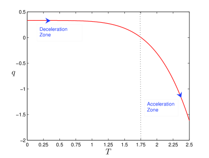
Figure 1: Plot of deceleration parameter $q$ versus time $T$.

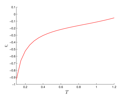
Figure 2: Plot of EoS parameter $\omega$ versus time $T$.

Hence the spacetime (1) is reduced to

$$ds^{2}=-\frac{dB^{2}}{n_{1}^{2}B^{-2(n+1)}\left(\frac{2\ell}{(k+1)}B^{\frac{k+1}{n_{1}}}+c_{1}\right)}+B^{2n}dx^{2}+B^{2}(dy^{2}+dz^{2}).$$ (18)

After using the suitable transformation of coordinates, $B=T$, the above model (18) transforms to

$$ds^{2}=-\frac{dT^{2}}{n_{1}^{2}T^{-2(n+1)}\left(\frac{2\ell}{(k+1)}T^{\frac{k+1}{n_{1}}}+c_{1}\right)}+T^{2n}dx^{2}+T^{2}(dy^{2}+dz^{2}).$$ (19)

It is to be noted that Eq. (17) indicates the explicit dependence of $B$ on $t$, i.e. $B=B(t)$. However, one can not solve Eq. (17) in general. So, in order to solve the problem completely, we have to choose either $B$ or $n$ in such a manner that (17) be integrable. It can be easily checked that different suitable values of $n$ generate the numerical solution of Eq. (17). But we are looking for a physically viable model of Universe and this prompt us to consider the transformation $B=f(t)=T$, which gives the time dependent DP. With this transformation Eq. (17) leads $t$ = constant for $T=0$.

Now, Eq. (15) yields

$$A=T^{n}.$$ (20)

It is important to note here that the derived model recovers isotropy with $n=1$. However, when we put $n=1$ in Eq. (16), it leads to a singularity. Therefore one can not choose $n=1$ to describe the feature of Universe in the present model.

The physical parameters such as the directional Hubble’s parameters $(H_{x},H_{y},H_{z})$, the average Hubble parameter $(H)$, the expansion scalar $(\theta)$, the spatial volume $(V)$ and the scale factor $(a)$ are, respectively given by

$$H_{x}=nn_{1}T^{-(n+2)}\sqrt{\frac{2\ell}{(k+1)}T^{\frac{(k+1)}{n_{1}}}+c_{1}},$$ (21)

$$H_{y}=H_{z}=n_{1}T^{-(n+2)}\sqrt{\frac{2\ell}{(k+1)}T^{\frac{(k+1)}{n_{1}}}+c_{1}},$$ (22)

$$H=\frac{1}{3}T^{-(n+2)}\sqrt{\frac{2\ell}{(k+1)}T^{\frac{(k+1)}{n_{1}}}+c_{1}},$$ (23)

$$\theta=3H=T^{-(n+2)}\sqrt{\frac{2\ell}{(k+1)}T^{\frac{(k+1)}{n_{1}}}+c_{1}},$$ (24)

$$V=T^{n+2},$$ (25)

$$a=T^{\frac{n+2}{3}}.$$ (26)

The value of DP $(q)$ is found to be

$$q=-1+\frac{1}{3}\left[\frac{\ell(k+3)}{k+1}T^{\frac{k+1}{n_{1}}}+c_{1}\right].$$ (27)

The sign of $q$ indicates whether the model inflates or not. A positive sign of $q$ corresponds to the standard decelerating model whereas the negative sign of $q$ indicates inflation. The recent observations of SN Ia Riess1998 ; Perlmutter1999 ; Torny2003 and CMB anisotropies Bennett2003 disclose that the expansion of the Universe is accelerating at present and it was decelerating in past with a transition redshift about $0.5$. It is therefore expected a signature flipping in the DP for the Universe which was decelerating in the past and is accelerating at the present time Padmanabhan2003 . In standard cosmology the DP naturally evolves with time just because there are many fluids, and whichever takes over determines it at any given time. However, recently Saha and Yadav Saha2011 presented an anisotropic DE model with time varying DP. In the present work, Fig. 1 depicts the variation of DP versus cosmic time as representative case with appropriate choice of constants of integration and other physical parameters.

The shear scalar $(\sigma)$ and the mean anisotropy parameter $(A_{m})$ are given by

$$\sigma^{2}=\frac{1}{18T^{2(n+2)}}\left[\left(1-\frac{1}{3nn_{1}}\right)^{2}+2\left(1-\frac{1}{3n_{1}}\right)^{2}\right]\left({\frac{2\ell}{(k+1)}T^{\frac{(k+1)}{n_{1}}}+c_{1}}\right)$$ (28)

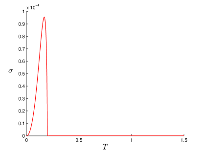
Figure 3: Plot of shear scalar $\sigma$ versus time $T$.

$$A_{m}=\frac{1}{3}\left[\left(1-\frac{1}{3nn_{1}}\right)^{2}+2\left(1-\frac{1}{3n_{1}}\right)^{2}\right]$$ (29)

The energy density of the cosmic fluid $(\rho)$, the EoS parameter $(\omega)$ and the energy density of magnetic fluid $(\rho_{B})$ are found to be

$$\rho=\frac{n_{1}^{2}\left(\frac{2\ell}{k+1}T^{\frac{k+1}{n_{1}}}+c_{1}\right)}{T^{2n+2}}\left[1+\frac{2n}{T}-\frac{\beta}{T^{4}}\right],$$ (30)

$$\omega=-\frac{\left[2n_{1}\ell T^{\frac{k+1}{n_{1}}-1}+(3T-2)T^{2n+1}-\beta T^{2n-2}\right]}{n_{1}^{2}\left(\frac{2\ell}{k+1}T^{\frac{k+1}{n_{1}}}+c_{1}\right)\left(1+\frac{2n}{T}-\frac{\beta}{T^{4}}\right)},$$ (31)

$$\rho_{B}=\frac{\beta}{T^{4}}.$$ (32)

The parameters $H$, $\theta$ and $\sigma^{2}$ start off with extremely large values and continue to decrease with the expansion of the Universe whereas the spatial volume $(V)$ grows with the cosmic time. Fig. 2 shows the variation of EoS parameter $(\omega)$ versus cosmic time for accelerating phase of the Universe as a representative case with appropriate choice of constants of integration and other physical parameters.

In the derived model the shear is limited to about $10^{-4}$ (Fig. 3) which is in fair agreement with the work of Adamek et al Adamek2011 .

4 Some Observational Constraint

In this section we follow the maximum likelihood approach under which one minimizes $\chi^{2}$ and hence measures the deviations of the theoretical predictions from the observations.

Let us now provide the scale factor $a$ and redshift $z$ are connected through the relation

$$a=\frac{a_{0}}{(1+z)},$$ (33)

where $a_{0}$ is the present value of scale factor.

Combining Eqs. (23), (26) and (33), one can easily obtain the expression for the Hubble’s parameter $(H)$ in terms of redshift parameter $(z)$ as follows

$$H=H_{0}(1+z)^{\frac{3(n+4)}{n+2}}.$$ (34)

Here $H_{0}$ is the present value of the Hubble’s parameter. Note that this relation is obtained by omitting the constant of integration.

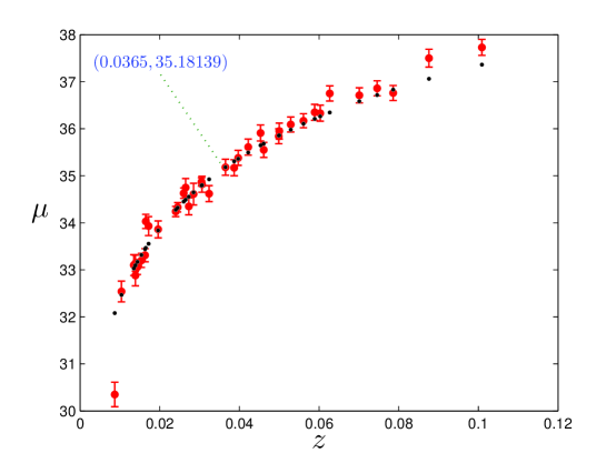
Figure 4: The distance modulus $\mu$ as function of redshift (z) to the derived model compared with SN Ia data from Amanullah et al. Amanullah2010 . The observational $\mu(z)$ data points are shown with error bars and the solid dots corresponds to distance modulus of derived model.

It is necessary for the investigation of type Ia supernovae to explore DE and constraint the models. Since SN Ia behave as excellent standard candles, they can be used to directly measure the expansion rate of the Universe upto high redshift, comparing with the present rate. The SN Ia data gives us the distance modulus $(\mu)$ to each supernova as

$$\mu=5log_{10}D_{L}(z)+\mu_{0},$$ (35)

where $D_{L}=\frac{H_{0}d_{L}}{c}$ is the Hubble-free luminosity distance and $\mu_{0}$ is the zero point offset, defined as

$$\mu_{0}=5log_{10}\left(\frac{cH_{0}^{-1}}{Mpc}\right)+25.$$ (36)

Inserting Eq. (36) into Eq. (35), we obtain

$$\mu=5log_{10}\left(\frac{d_{L}}{Mpc}\right)+25.$$ (37)

The luminosity distance $(d_{L)}$ is calculated by

$$d_{L}=r_{1}(1+z)a_{0}.$$ (38)

For the determination of $r_{1}$, we assume that a photon emitted by a source with co-ordinate $(r,t)$ and received at a time $t_{0}$ by an observer located at $r=0$. Then we determine $r_{1}$ from following relation

$$r_{1}=\int^{t_{0}}_{t}\frac{dt}{a}.$$ (39)

By solving the Eqs. (37)$-$(39) and (26), one can easily obtain the expression for distance modulus $(\mu)$ in the term of red shift parameter $(z)$ as

$$\mu=5log_{10}\left[\frac{3H_{0}^{\frac{1}{(n+2)k}}(1+z)^{\frac{2n+1}{n+2}}}{{\sqrt{\frac{2\ell}{k+1}}}^{\frac{1}{(n+2)k}}}\left((1+z)^{\frac{1-n}{n+2}}-1\right)\right]+25,$$ (40)

where $H_{0}$ is in the unit of Km $s^{-1}$Mp$c^{-1}$.

Table 1: Comparison of the results of present model with the observational data

Redshift$(z)$	Supernovae Ia$(\mu^{data})$	Our model $(\mu^{th})$
0.0087	$30.35^{+0.26}_{-0.26}$	32.07943
0.0104	$32.54^{+0.22}_{-0.22}$	32.46627
0.0135	$33.10^{+0.22}_{-0.22}$	33.031435
0.0172	$33.93^{+0.2}_{-0.2}$	33.555816
0.0245	$34.33^{+0.1}_{-0.01}$	34.320871
0.0285	$34.61^{+0.23}_{-0.23}$	34.64755
0.0306	$34.82^{+0.17}_{-0.17}$	34.8010
0.0365	$35.18^{+0.17}_{-0.17}$	35.18139
0.0453	$35.91^{+0.17}_{-0.17}$	35.64668
0.0499	$35.84^{+0.16}_{-0.16}$	35.85475
0.0529	$36.09^{+0.16}_{-0.16}$	35.98026
0.0589	$36.35^{+0.17}_{-0.17}$	36.21104
0.0603	$36.33^{+0.17}_{-0.17}$	36.26146
0.0627	$36.75^{+0.16}_{-0.16}$	36.34521
0.0701	$36.71^{+0.16}_{-0.16}$	36.58437
0.0746	$36.86^{+0.16}_{-0.16}$	36.71760
0.0786	$36.76^{+0.16}_{-0.16}$	36.82936
0.0876	$37.5^{+0.19}_{-0.19}$	37.06104
0.1009	$37.73^{+0.17}_{-0.17}$	37.36251

In the present analysis, we use $19$ data set out of recently released $38$ data set of SN Ia in the range $0.0015\leq z<0.12$, as reported by Amanullah et al. Amanullah2010 (Table 1). In this case $\chi_{SN}^{2}$ has been computed according to the following relation

$$\chi_{SN}^{2}=A-\frac{B^{2}}{C}+log_{10}\left(\frac{C}{2\pi}\right)=97.772,$$ (41)

where

$$A=\sum_{i}^{38}\frac{\left(\mu^{data}-\mu^{th}\right)^{2}}{\sigma_{i}^{2}},$$

$$B=\sum_{i}^{38}\frac{\left(\mu^{data}-\mu^{th}\right)}{\sigma_{i}^{2}},$$

$$C=\sum_{i}^{38}\frac{1}{\sigma_{i}^{2}}.$$

The comparison between distance modulus $\mu$ of the derived model and the observational $\mu(z)$ SN Ia data as reported by Amanullah et al. Amanullah2010 can be seen in Fig. 4. The observational $\mu(z)$ data points are shown with error bars and the solid dots corresponds to distance modulus of the derived model. It is observed that the derived model is fit well with SN Ia observation (see Fig. 4). Note that the best fit value of distance modulus is $\mu(z\;=\;0.0365)=35.18139$ with $\chi_{SN}^{2}=97.772$ and the reduced $\chi^{2}$ value is $\chi_{SN}^{2}$/(degree of freedom)=2.64.

5 Results and Discussions

In this paper, we have investigated magnetized DE model under the assumption that $\sigma\propto\theta$ in Bianchi-I spacetime. Under some specific choice of the parameters the present consideration yields the time dependent DP and EoS parameters. It is to be noted that our procedure of solving the field equations are altogether different from what Sharif and Zubair Sharif2010 have adopted. The derived model starts expanding with Big Bang singularity at $T=0$ and this singularity is point type because the directional scale factors $A$ and $B$ both simultaneously vanish at $T=0$. The dynamics of DP parameter yields two different phases of the Universe. Initially DP is evolving with positive sign that yields the decelerating phase of the Universe whereas in the later times it is evolving with negative sign which describes the present phase of the acceleration of the Universe. Thus the derived model has transition of the Universe from the early deceleration phase to the later acceleration phase which is in good agreement with the recent observations Caldwell2006 .

The distance modulus of the derived model fit well with the observational $\mu(z)$ values (see Fig. 4 and Table 1) which in turn imply that the derived model is physically realistic. It is important to note here that in the absence of the magnetic field only the anisotropic distribution of DE leads the present acceleration of the Universe Yadav2011c while in the presence of magnetic field along with the isotropic distribution of DE describes the dynamics of the Universe from Big Bang to the present epoch. Thus the magnetic field isotropizes the distribution of DE which signifies the role of magnetic field. Hence from the theoretical perspective, the present model can be a viable model to explain the late time acceleration of the Universe. In other words, the solution presented here can be one of the potential candidates to describe the observed Universe.

It is worth noticing that we have presented solutions of a magnetized Bianchi-I Universe like King and Coles King2007 . However, their work is concerned with vacuum energy. In our case, we have studied the Universe consists of cosmic fluid with equation of state $w=p/\rho$. Therefore, our study is more general than King and Coles King2007 .

In the present work we observe an interesting feature that the magnetic presence isotropises the expansion in the model. However, it is not clear, in particular, what property of the magnetic field is responsible for the isotropisation. Is it the additional energy density of the field, is it the magnetic pressure, or maybe the tension? It can be observed that the solution of Eq. (16) does not exist for $n=1$. Therefore, in the derived model, one can not choose $n=1$. To obtain an explicit solution of Eq. (16), one can choose $\beta=0$ which leads to $\rho_{B}=0$ and the isotropic distribution of cosmic fluid. This can also be observed from the LHS’s of Eqs. (4) and (5), which are same for $n=1$. As a result, one should get $\rho_{B}=0$. This means, there is no contribution of magnetic field and the model becomes an isotropic FRW model. The well known criteria for isotropization are $A=\frac{1}{3}\Sigma\frac{H_{i}^{2}}{H^{2}}-1\rightarrow 0$ and $\Sigma^{2}=\frac{1}{2}AH^{2}-1\rightarrow 0$, where $A$, $\Sigma^{2}$ are average anisotropy and shear respectively, and $H_{i}^{2}$ is the directional Hubble parameter. Obviously, these criteria are valid for large physical time. In the present model (Eqs. (21) - (24)), one can easily find out that for large time, $A\rightarrow\frac{2(n-1)^{2}}{n+2)^{2}}$ and $\Sigma^{2}\rightarrow 0$. This immediately implies that for $n\rightarrow 1$ our model turns out to be an isotropic FRW model. Therefore, $n=1$ is the condition of isotropy in the absence of magnetic field and the presence of magnetic field has constraint on $n=1$. This seems to contribute the magnetic field which resembles with the initial anisotropy of the Universe. With the passage of time magnetic field decreases and becomes negligible at late time to approach towards isotropy.

Our solution, in the present investigation, shows that the constrained equation of state of $\rho$ evolves in time, but this is not all that is needed when comparing with observations. This explicitly means that it is not exactly known about the generic fluid $\rho$, and how does it describe and include the known cosmological history where an early radiation domination gave way to matter domination. In particular, fitting the $H(z)$ evolution law derived from SN observations is only one of the many pieces of information which need to be used. A thorough discussion of all basic cosmological constraints is beyond the scope of this analysis in the present paper and is awaiting for a future project.

References

- (1) A.G. Riess et al., AJ 116, 1009 (1998).
- (2) S. Perlmutter et al., ApJ 517, 565 (1999).
- (3) A.C. Pope et al., ApJ 607, 655 (2004).
- (4) R.R. Caldwell, W. Komp, L. Parker, D.A.T. Vanzella, PRD 73, 023513 (2006).
- (5) S. Carroll, Liv. Rev. Relativ. 4, 1 (2001).
- (6) P.J.E. Peebles, B. Ratra, Rev. Mod. Phys. 75, 559 (2003).
- (7) J.M. Overduin, F.I. Cooperstock, PRD 58, 043506 (1998.
- (8) P.J. Steinhardt, L.M. Wang, I. Zlatev, PRD 59, 123504 (1999).
- (9) R.R. Caldwell, PLB 545, 23 (2002).
- (10) A.G. Riess et al., AJ 607, 665 (2004).
- (11) P. Astier et al., A & A 447, 31 (2006).
- (12) D.J. Eisentein et al., ApJ 633, 560 (2005).
- (13) C.J. MacTavish et al., ApJ 647, 799 (2006).
- (14) E. Komatsu et al., ApJ Suppl. Ser. 180, 330 (2009).
- (15) G. Hinshaw et al., ApJ Suppl. 180, 225 (2009).
- (16) G. Hinshaw et al., ApJ Suppl. 148, 135 (2003).
- (17) J. Jaffe et al., ApJ 629, L1 (2005).
- (18) J. Jaffe et al., ApJ 643, 616 (2006a).
- (19) J. Jaffe et al., A & A 460, 393 (2006b).
- (20) L. Campanelli, P. Cea, L. Tedesco, PRL 97, 131302 (2006).
- (21) L. Campanelli, P. Cea, L. Tedesco, PRD 76, 063007 (2007).
- (22) W. Huang, J. Math. Phys. 31, 1456 (1990).
- (23) L.P. Chimento et al., CQG 14, 3363 (1997).
- (24) J.A.S. Lima, M. Trodden, PRD 53, 4280 (1996).
- (25) J.A.S. Lima, J.M.F. Maia, PRD 49, 5597 (1994).
- (26) A. Pradhan, S.K. Singh, Int. J. Mod. Phys. D 13, 503 (2004).
- (27) B. Saha, Astrophys. Space Sci. 302, 83 (2006a).
- (28) B. Saha, Int. J. Theor. Phys. 45, 983 (2006b).
- (29) R. Battye, A. Moss, PRD 80, 023531 (2009).
- (30) L. Campanelli, P. Cea, G.L. Fogli, L. Tedesco, PRD 81, 081301 (2010).
- (31) S. Appleby, R. Battye, A. Moss, Int. J. Mod. Phys. D 20, 1153 (2011).
- (32) O. Akarsu, C.B. Kilinc, GRG 42, 119 (2010).
- (33) S. Kumar, A.K. Yadav, Mod. Phys. Lett. A 26, 647 (2011).
- (34) H. Amirhashchi, A. Pradhan, B. Saha, Astrophys. Space Sci. 333, 295 (2011).
- (35) A.K. Yadav, L. Yadav, Int. J. Theor. Phys. 50, 218 (2011).
- (36) A.K. Yadav, F. Rahaman, S. Ray, Int. J. Theor. Phys. 50, 871 (2011).
- (37) A.K. Yadav, B. Saha, Astrophys. Space Sci. DoI: 10.1007/s10509-011-0861-0 (2011).
- (38) A.K. Yadav, Astrophys. Space Sci. 335, 565 (2011).
- (39) E.J. King, P. Coles, CQG 24, 2061 (2007).
- (40) J.D. Barrow, P.G. Ferreira, J. Silk, PRL 78, 3610 (1997).
- (41) K.T. Kim, P.C. Tribble, P.P. Kronberg, ApJ 379, 80 (1991).
- (42) R. Perley, G. Taylor, AJ 101, 1623 (1991).
- (43) P.P. Kronberg, Rep. Prog. Phys., 57, 325 (1994).
- (44) P.P. Kronberg, J.J. Perry, E.L. Zukowski, ApJ 387, 528 (1992).
- (45) A. M. Wolfe, K. Lanzetta, A.L. Oren, ApJ 388, 17 (1992).
- (46) D. Grasso, H.R. Rubinstein, Astropart. Phys. 3, 95 (1995).
- (47) K.S. Thorne, ApJ 148, 51 (1967).
- (48) A.G. Doroshkevich, Astrophys. 1, 138 (1965).
- (49) K.C. Jacobs, ApJ 155, 379 (1969).
- (50) M.S. Maden, MNRAS 237, 109 (1989).
- (51) E. Milaneschi, R. Fabbri, A & A 151, 7 (1985).
- (52) V.G. LeBlanc, CQG 14, 2281 (1997).
- (53) C.G. Tsagas, R. Maartens, CQG 17, 2215 (2000).
- (54) M. Sharif, M. Zubair, Astrophys. Space Sci. 330, 399 (2010).
- (55) S.M. Carroll, M. Hoffman, M. Trodden, PRD 68, 023509 (2003).
- (56) R. Kantowski, R.K. Sachs, J. Math. Phys. 7, 443 (1966).
- (57) J. Kristian, R.K. Sachs, ApJ 143, 379, (1966).
- (58) C.B. Collins, E.N. Glass, D.A. Wilkinson, GRG 12, 805 (1980).
- (59) J.L. Torny et al., ApJ 594, 1 (2003).
- (60) C.L. Bennett et al., ApJ Suppl. Ser. 148, 1 (2003).
- (61) T. Padmanabhan, T. Roychowdhury, MNRAS 344, 823 (2003).
- (62) B. Saha, A.K. Yadav, Astrophys. Space Sci. DOI: 10.1007/s10509-012-1070-1; arXiv: 1110.4887 [physics.gen-ph] (2011).
- (63) J. Adamek, R. Durrer, E. Fenu, M. Vanlanthen, JCAP 06, 017 (2011).
- (64) R. Amanullah et al., ApJ 716, 712 (2010).