Are there nodes in LaFePO, BaFe₂(AsP)₂, and KFe₂As₂ ?

Abstract

We reexamined the experimental evidences for the possible existence of the superconducting (SC) gap nodes in the three most suspected Fe-pnictide SC compounds: LaFePO, BaFe₂(As_0.67P_0.33)₂, and KFe₂As₂. We showed that while the $T$-linear temperature dependence of the penetration depth $\lambda(T)$ of these three compounds indicate extremely clean nodal gap superconductors, the thermal conductivity data $\lim_{T,H\rightarrow 0}\kappa_{S}(H,T)/T$ unambiguously showed that LaFePO and BaFe₂(As_0.67P_0.33)₂ are extremely dirty, while KFe₂As₂ can possibly be clean. This apparently conflicting experimental data casts a serious doubt on the nodal gap possibility on LaFePO and BaFe₂(As_0.67P_0.33)₂.

1 Introduction

Despite the intensive research effort since the discovery of the Fe-based superconductors, [1] the pairing symmetry of this new class of superconducting (SC) compounds has not yet been settled. Early theories and experiments appear to best support the sign changing $s$-wave pairing state (denoted as $s_{\pm}$-, $s^{\pm}$-, or $\pm s$-state in the literature). [2, 3, 4, 5, 6] However, there exist several Fe-pnictide compounds that are not seemingly compatible with the $\pm$s state but are strongly suggesting for the presence of nodes in their SC states. Among others, LaFePO, [7, 8] BaFe₂(As_0.67P_0.33)₂,[9] and KFe₂As₂ [10] are the most compelling compounds for the nodal gap, and in lesser degree Ba(Fe_1-xCo_x)₂As₂ [11] is also suspected.

Commonly taken evidences for the nodal gap in the above mentioned compounds are: (1) $T$-linear temperature dependence of penetration depth $\lambda(T)$ down to very low temperatures,[7, 8, 9, 10] and (2) a strong field dependence in the thermal conductivity slope $\lim_{T\rightarrow 0}\kappa(H,T)/T$, which is proportional to in between $\sqrt{H}$ and $H$, accompanied with a substantial fraction of the residual thermal conductivity $\lim_{T,H\rightarrow 0}\kappa(H,T)/T=\kappa_{s0}/T$. [9, 12, 13, 14] These features are the well known signatures of the nodal gap superconductors such as the $d$-wave superconductivity of the high-$T_{c}$ cuprates. And although it was recently shown that the strong field dependence of the thermal conductivity $\kappa(H,T\rightarrow 0)$ can be equally well explained with the $\pm$$s$-wave state, [15] the extremely close $T$-linear $\lambda(T)$ is hard to be reconciled with other than a clean nodal gap superconductor. Furthermore, the finite value of the residual thermal conductivity $\kappa_{s0}/T$ measured in all three compounds [9, 12, 13, 14] –it is known that the nodal gap SC state produces an universal thermal conductivity slope independent of the amount of impurity concentrations [16, 17, 18] – is another evidence for a nodal gap state, so it was widely interpreted to support the presence of nodes in these compounds together with the penetration depth data.

In this paper, however, we will show that there is a serious and unreconcilable conflict between the above mentioned two experimental evidences for the nodal gap. We notice that (1) the universal value of $\kappa_{S0}/T$ delivers no information about the dirtiness of the superconducting sample, however, (2) the normal state value of $\kappa_{N}/T$ tells us the amount of dirts in the sample. Then combining the facts (1) and (2), the ratio $\kappa_{S}/\kappa_{N}$, which is usually plotted data in experiments, is a very good indicator of the dirtiness of the sample. Inspecting the reported data of thermal conductivities of the three compounds, we concluded that the measured samples of LaFePO and BaFe₂(As_0.67P${}_{0.33})_{2}$ should have a large amount of impurities and hence cannot be compatible of the $T$-linear $\lambda(T)$ within the nodal gap scenario. In the case of KFe₂As₂, there exist two very different thermal conductivity data by Dong et al.[13] and Reid et al.[14] with different $T_{c}$ samples, 3K and 3.8K, respectively. Our analysis of the thermal conductivity data showed that the sample of [14] ($T_{c}\sim 3.8$K) is cleaner with at least 10 times less impurity concentration than the sample of Ref.[13] ($T_{c}\sim 3$K). Hence, the former sample of KFe₂As₂ can possibly be compatible with the $T$-linear $\lambda(T)$ data. We conclude that KFe₂As₂ can remain a possible nodal gap superconductor, but not LaFePO and BaFe₂(As_0.67P${}_{0.33})_{2}$.

2 Theory

Assuming the quasiparticle excitation $E({\bf k})=\sqrt{(v_{1}k_{1})^{2}+(v_{F}k_{2})^{2}}$ in the $d$-wave superconductor ($v_{F}$ Fermi velocity perpendicular to the Fermi surface(FS), $v_{1}$ nodal gap velocity parallel to the FS), the universal thermal (electric) conductivity in the nodal gap superconductor has been derived as follows.[16, 17, 18]

$$\frac{\kappa_{S}(T=0)}{T} \sim v_{F}^{2}\int dk_{1}dk_{2}\frac{\gamma_{s}^{2}}{[\gamma_{s}^{2}+(v_{1}k_{1})^{2}+(v_{F}k_{2})^{2}]^{2}}$$ (1)

$$= \frac{v_{F}^{2}}{v_{F}v_{1}}\frac{\Delta_{0}}{\sqrt{\gamma_{s}^{2}+\Delta_{0}^{2}}},$$

where $\Delta_{0}$ is the maximum gap value of the $d$-wave gap $\Delta(\theta)$ and $\gamma_{s}$ is the impurity induced damping rate at zero energy in the SC state. As well known, $\frac{\kappa_{S}}{T}$ indeed becomes universal, independent of the impurity concentrations and scattering strength, but only in the limit of $\Delta_{0}\gg\gamma_{s}$; Eq.(1) clearly shows that a deviation occurs when $\gamma_{s}\sim\Delta_{0}$. The normal state limit of the above is easy to derive as

$$\frac{\kappa_{N}(T=0)}{T} \sim \frac{v_{F}^{2}}{v_{F}v_{1}}\frac{\Delta_{0}}{\gamma_{n}},$$ (2)

where $\gamma_{n}$ is the impurity induced damping rate in the normal state and in general $\gamma_{s}\neq\gamma_{n}$ for the same impurity strength and concentration. Knowing that the normal state should have no memory of the superconductivity, the above expression of $\frac{\kappa_{N}}{T}$ is a disguised form for convenient comparison with Eq.(1) and $\frac{\Delta_{0}}{v_{1}}$ becomes $\pi/4$ or a momentum scale of the FS size. Also we don’t need to know the material specific parameters like $N(0),v_{F}$, etc to estimate the absolute magnitude of the thermal conductivities because for our purpose we only need the ratio

$$\frac{\kappa_{S}}{\kappa_{N}} = \frac{\gamma_{n}}{\sqrt{\gamma_{s}^{2}+\Delta_{0}^{2}}}$$ (3)

$$= \frac{\Gamma}{\Delta_{0}}\frac{1}{\sqrt{1+\Gamma/\Delta_{0}}}\approx\frac{\Gamma}{\Delta_{0}}.$$ (4)

where $\Gamma=n_{imp}/\pi N(0)$ is the impurity concentration parameter and in the second line of the above equations we used the results of $\gamma_{s}\approx\sqrt{\Delta_{0}\Gamma}$ and $\gamma_{n}=\Gamma$ assuming the unitary impurity scattering strength. Eq.(4) is the key result of this paper.

It was nice to observe the universal value of the thermal conductivity slope $\kappa_{S}/T$ of Eq.(1) to confirm a nodal superconductor. On the other hand, it was also a drawback since the universal thermal conductivity slope doesn’t tell us how dirty or clean the sample is. However, as shown in Eq.(4), the ratio $\kappa_{S}/\kappa_{N}$ is an excellent indicator of the dirtiness of the specific SC sample. At this point, we would like to recall the fact that the typical experimental values of $\kappa_{S}/\kappa_{N}$ measured in LaFePO and BaFe₂(As_0.67P_0.33)₂ are $\frac{\Gamma}{\Delta_{0}}\approx 0.2-0.4$ which is quite high level of impurity concentration for a nodal gap superconductor.

3 Numerical calculations and discussions

In this section we will show the full numerical calculations of the field dependence of $\lim_{T\rightarrow 0}\kappa_{S}(H,T)/T$ as well as the specific coefficient $\lim_{T\rightarrow 0}C(H,T)/T$ of the canonical $d$-wave gap ($\Delta(\theta)=\Delta_{0}\cos{2\theta}$) state with the various impurity concentrations. Also the results of the penetration depth $\lambda(T)$ will be shown for the corresponding impurity concentrations.

To calculate the field dependencies of the thermal conductivity and specific heat in the mixed state with applied field, we just need to calculate the position dependent DOS $N(\omega,r)$ in the presence of vortices. In the semiclassical approximation, the matrix form of the single-particle Green’s function in the SC state, including Doppler shift of the quasiparticle excitations $\epsilon(k)$ due to the circulating supercurrent ${\bf v_{s}(r)}$, is given by [15, 19, 20]

$$\hat{G}({\bf k,r,\omega,\theta})=\frac{[\omega+{\bf v_{s}(r)}\cdot{\bf k}]\tau_{0}+\epsilon(k)\tau_{3}+\Delta_{\theta}\tau_{1}}{[\omega+{\bf v_{s}(r)}\cdot{\bf k}]^{2}-\epsilon^{2}(k)-\Delta^{2}_{\theta}}$$ (5)

where $\tau_{i}$ are Pauli matrices and the supercurrent velocity around the vortex core ${\bf v_{s}(r)}$ is $\sim\frac{1}{m}\frac{1}{r}{\bf\hat{\theta}}$, with ${\bf r}$ the distance from the vortex core. The position dependent DOS is calculated as $N(\omega,r)=-\frac{1}{\pi}{\rm TrIm}\sum_{k}\int d\theta~{}G_{0}({\bf k,r,\omega,\theta})$. Finally, the field dependent quantities are obtained from the areal average DOS per unit volume as $\bar{N}(\omega,H)=\int_{\xi}^{R_{H}}dr^{2}N(\omega,r)/\pi R_{H}^{2}$ with the magnetic length $R_{H}=\sqrt{\frac{\Phi_{0}}{\pi H}}$ ($\Phi_{0}$ a flux quanta) and the SC coherence length $\xi$.

The impurity scattering is included by the $\mathcal{T}$-matrix method. [21, 22, 23] The impurity induced self-energies renormalize the frequency and order parameter (OP) as $\omega\rightarrow\tilde{\omega}=\omega+\Sigma^{0}(\omega)$ and $\Delta_{0}\rightarrow\tilde{\Delta}_{0}=\Delta_{0}+\Sigma^{1}(\omega),$ with $\Sigma^{0,1}(\omega)=\Gamma\cdot\mathcal{T}^{0,1}(\omega)$, where $\mathcal{T}^{0,1}$ are the Pauli matrices $\tau^{0,1}$ components of the $\mathcal{T}$-matrices in the Nambu space. However, $\mathcal{T}^{1}$ is identically zero in the $d$-wave state. Then all impurity effect and the Volovik effect can be incorporated into the local Green’s function Eq.(5) by replacing $\omega$ by $\tilde{\omega}$.

After calculating the averaged $\bar{N}(\omega,H)$ for all frequencies, specific heat is calculated as

$$C(T,H)=\int_{0}^{\infty}d\omega(\frac{\omega}{T})^{2}\frac{\bar{N}(\omega,H)}{{\rm cosh}^{2}(\frac{\omega}{2T})}$$ (6)

Similarly, thermal conductivity is calculated by [24]

$$\kappa(T,H,r)\propto v_{F}^{2}\int d\theta\int_{0}^{\infty}d\omega(\frac{\omega}{T})^{2}\frac{K(\omega,H,r,\theta)}{{\rm cosh}^{2}(\frac{\omega}{2T})}$$ (7)

with

$$K(\omega,H,r,\theta)=\frac{1}{Im\sqrt{\tilde{z}^{2}-\Delta^{2}_{\theta}}}\times\Big{(}1+\frac{|\tilde{z}|^{2}-|\Delta_{\theta}|^{2}}{|\tilde{z}^{2}-\Delta^{2}_{\theta}|}\Big{)}$$ (8)

where $\tilde{z}=\tilde{\omega}+{\bf v}_{s}({\bf r)}\cdot{\bf k_{F}}$. And the longitudinal and transversal thermal conductivities are calculated as $\kappa_{\parallel}(T,H)=\int_{\xi}^{R_{H}}d^{2}r\kappa(T,H,r)/\pi R_{H}^{2}$ and $\kappa^{-1}_{\perp}(T,H)=\int_{\xi}^{R_{H}}d^{2}r\kappa^{-1}(T,H,r)/\pi R_{H}^{2}$, respectively.

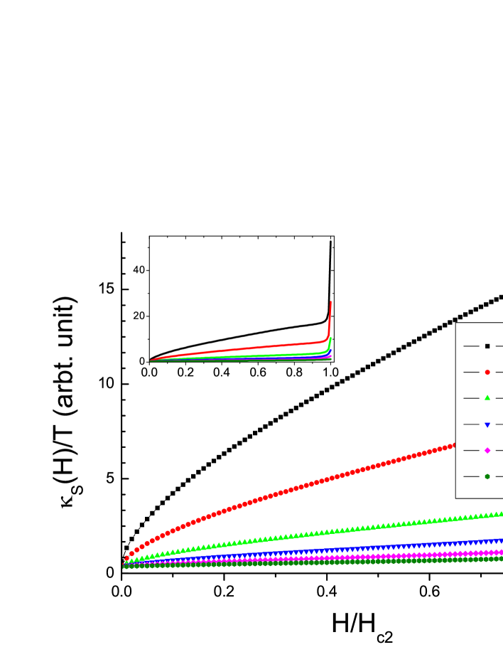
Figure 1: (Color online) Thermal conductivity $\kappa_{S}(H)/T$ vs the normalized fields $H/H_{c2}$ of the $d$-wave SC state, calculated at $T=0.02\Delta_{0}$ for various impurity concentrations $\Gamma/\Delta_{0}=0.01,0.02,0.05,0.1,0.2,$ and 0.4. (unitary impurity). The inset shows the full range of fields up to $H/H_{c2}=1$.

3.1 Thermal conductivity

Figure 1 shows the theoretical thermal conductivity $\kappa(T,H)/T$ vs $H$ of the $d$-wave SC state calculated at the low temperature limit of $T/\Delta_{0}=1/50$ with the varying impurity concentrations of the unitary scatterers, $\Gamma/\Delta_{0}=0.01,0.02,0.05,0.1,0.2,$ and 0.4. First, the results indeed showed that the universal thermal conductivity $\lim_{T,H\rightarrow 0}\kappa(T,H)/T$ is well reproduced by our numerical calculations for the vast range of impurity concentrations. Second, it showed that the normal state limit of $\kappa(T,H)/T$, which is approached by increasing the field strength $H$ toward $H_{c2}$, is inversely proportional to the impurity concentration as shown in Eq.(4). The inset shows the results for the full range of $H/H_{c2}=[0:1]$ and we can see that $\kappa(H)/T$ sharply increases near $H_{c2}$. This is due to a rapid collapse of the gap $\Delta_{0}(H)$ towards $H_{c2}$ and our semiclassical approximation faithfully follows the Doppler shifting effect of this rapidly collapsing gap up to $H_{c2}$. While this is the correct calculation results with the semiclassical approximation, it is also known that this semiclassical approximation is not precisely correct near $H_{c2}$ where the quantum effect should become important.[25] So the exact field dependence of $\kappa(T,H)/T$ near $H_{c2}$ in Fig.1 should not be taken seriously.

However, the important points for our purpose are: (1) at both limits, the universal limit value of $\lim_{T,H\rightarrow 0}\kappa(T,H)/T$ and the normal state limit value $\kappa(H=H_{c2})/T$ are exact, and (2) the overall field dependence of the initially slow rise and then a rapid rise of $\kappa(H)/T$ near $H_{c2}$ is the genuinely correct behavior regardless of different theoretical treatments. [26] The main conclusions of this paper relies only on these two points. The main panel in Fig.1 shows the results for the limited region of $H\leq 0.9H_{c2}$ for a better resolution of the low field behavior of $\kappa_{S}(H)/T$.

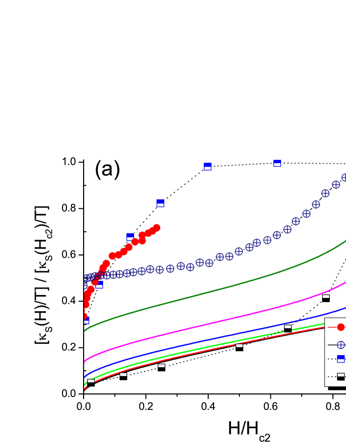
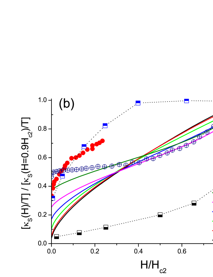
Figure 2: (Color online) (a) Theoretical thermal conductivities (lines) of Fig.1 normalized by the values of $\kappa_{S}(H_{c2})/T$ for each impurity concentrations $\Gamma/\Delta_{0}=0.01,0.02,0.05,0.1,0.2,$ and 0.4. (the same colors as in Fig.1). Symbols are the cropped data of experiments. (b) The same data as in (a) but normalized by the values of $\kappa_{S}(H=0.9H_{c2})/T$ for each impurity concentration. Symbols are the same as in (a).

In Fig.2, we replotted the theoretical results of Fig.1 with two different normalizations and the experimental data of $[\kappa_{S}(H)/T]/[\kappa_{N}/T]$ are overlaid. Fig.2(a) normalized $\kappa_{S}(H)/T$ of Fig.1 with its $\kappa_{S}(H=H_{c2})/T$ values for each impurity concentration, and Fig.2(b) used the $\kappa_{S}(H=0.9H_{c2})/T$ values for normalization. The second normalization plot by the $H=0.9H_{c2}$ values was chosen because it is the typical point of saturation before the sharp rise as seen in the inset of Fig.1. and this concave-down saturation behavior approaching $H_{c2}$ is the typical observations in experiments. [9, 12, 13] Different normalizations yield different line shapes of the normalized $\kappa_{S}(H)/T$ which is supposed to be compared to the experimental $[\kappa_{S}(H)/T]/[\kappa_{N}/T]$. The true behavior should be somewhere in between Fig.2(a) and Fig.2(b), but we emphasize that this fine detail is irrelevant to our main conclusions and analysis. The overlayed experimental data are BaFe₂(As_0.67P_0.33)₂, [9] LaFePO, [12] and KFe₂As₂. [13, 14]

Regardless of the choice of the normalizations, the experimental values of the residual thermal conductivity of BaFe₂(As_0.67P_0.33)₂, [9] LaFePO, [12] and KFe₂As₂ [13] unambiguously indicate that these compounds should have the impurity concentration $\Gamma/\Delta_{0}>0.4$, which is extremely dirty superconductor. Our theoretical calculations are with a single $d$-wave gap band. In reality, if there exists a nodal gap in these multiband Fe-pnictide compounds, the total gap function should consist of a nodal gap $+$ one or two $s$-wave gaps, for example, a nodal $\pm s$-wave gap.[12] If that is the case, the total $\kappa_{N}/T$ should increase due to the addition contributions from other bands. However, these additional $s$-wave gap bands have negligible contributions to the residual thermal conductivity $\lim_{T,H\rightarrow 0}\kappa_{S}(H)/T$ because they are fully gapped at low fields and low temperatures. Therefore, we need to have even higher impurity concentration than $\Gamma/\Delta_{0}>0.4$ in order to match the experimental data[9, 12, 13] of the normalized residual thermal conductivity $\lim_{H,T\rightarrow 0}[\kappa_{S}(H)/T]/[\kappa_{N}/T]$.

On the other hand, the data of KFe₂As₂ by Reid et al. [14] is very different from the data of KFe₂As₂ by Dong et al. [13] We can see that the data of Reid et al. [14] reasonably fit the theoretical result in Fig.2(a) with the impurity concentration, $\Gamma/\Delta_{0}<0.02$, which is relatively clean limit. As discussed in Ref.[14], the discrepancy between the data of two groups is understood by the sample purity. Judging from the $T_{c}$ of two samples (3.80K and 3K, respectively) and our theoretical calculations of $\kappa_{S}/\kappa_{N}$ in Fig.2, the sample of Reid et al. must be much cleaner, by about 10-20 times, than the one of Dong et al. and it appears to be consistent with the result of the clean d-wave calculation with $\Gamma/\Delta_{0}<0.02$ in Fig.2(a).

Summarizing the cases of BaFe₂(As_0.67P_0.33)₂ [9] and LaFePO [12], if we interpret the thermal conductivity data of these two compounds with a nodal gap scenario, we are led to conclude that both compounds are very dirty nodal gap superconductors. However, if this is true, the linear-$T$ penetration depth measurements[7, 8, 9] of these two compounds are in a serious conflict with the dirty nodal gap scenario.

In the case of KFe₂As₂, we have two seemingly contradicting thermal conductivity measurements [13, 14] as seen in Fig.2(a) and (b). However, despite the large difference of $T_{c}$ and the line shapes of $\kappa_{S}(H)/\kappa_{N}$, both samples reported a similar value of the residual thermal conductivity: $\kappa_{S0}/T$=3.7 $\pm$ 0.4 mW/K²cm (Ref.[14]) and $\kappa_{S0}/T$=2.27 $\pm$ 0.02 mW/K²cm (Ref.[13], here we ignored the correction by geometric factor discussed in Ref.[14]), respectively. This fact itself is a strong supporting evidence for the nodal gap in KFe₂As₂ compound. The different zero field intercepts of the data of two samples in Fig.2 are due to the normalization by the normal state thermal conductivities: $\kappa_{N}/T$=7.36 $\pm$ 0.04 mW/K²cm for Dong et al. [13] and $\kappa_{N}/T\approx$ 109 mW/K²cm for Reid et al. [14] The data of Reid et al.[14] can fit reasonably well with the clean nodal gap calculation ($\Gamma/\Delta_{0}<0.02$) for the most of low field region as seen in Fig.2(a). The data of Dong et al.,[13] however, doesn’t fit with any calculational results in Fig.2. While the residual thermal conductivity value of it can be fit with a dirty nodal gap with $\Gamma/\Delta_{0}\approx 0.4$, the data for $H>0$ increases much rapidly at low fields and saturates to become flat for $H>0.4H_{c2}$, not even close to any theoretical results in Fig.2. But, if we assume the additional bands with $s$-wave gaps in addition to a nodal gap, as in a nodal $\pm s$-wave state, it would be possible to fit the data of both clean and dirty limits of Ref.[13, 14]. The detailed SC properties of the nodal $\pm s$-wave state will be reported in future publication.

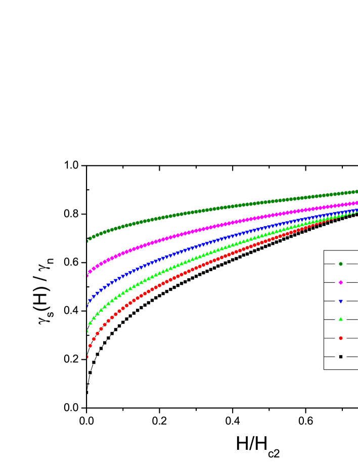
Figure 3: (Color online) Normalized specific heat coefficient $\lim_{T\rightarrow 0}C(T,H)/T=\gamma_{S}(H)$ vs fields $H/H_{c2}$ calculated at $T=0.02\Delta_{0}$ of the $d$-wave SC state for various impurity concentrations $\Gamma/\Delta_{0}=0,0.02,0.05,0.1,0.2,$ and 0.4 (unitary impurity).

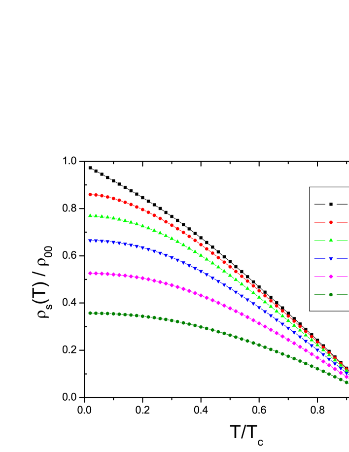
Figure 4: (Color online) Normalized superfluid density $\rho_{S}(T)$ vs $T/T_{c}$ of the $d$-wave SC state for various impurity concentrations $\Gamma/\Delta_{0}=0,0.02,0.05,0.1,0.2,$ and 0.4 (unitary impurity). $2\Delta_{0}/T_{c}=4$ is used.

3.2 Specific heat coefficient and Superfluid density

To foster the above discussions, we calculated the field dependence of the specific heat coefficient $\gamma_{s}(H)=\lim_{T\rightarrow 0}C(H,T)/T$ and the temperature dependence of the superfluid density $\rho(T)\sim 1/\lambda^{2}(T)$ of the $d$-wave state with various concentrations of the unitary impurities as in Figs.1 and 2. Figure 3 is the normalized $\gamma_{s}(H)/\gamma_{n}$ for $\Gamma/\Delta_{0}=0.4,0.2,0.1,0.05,0.02,$ and 0 (no impurity limit). It shows the expected behavior as the $\sqrt{H}$ behavior of $\gamma_{s}(H)$ in the clean limit becomes flattened with increasing the impurity concentration. The only point that we want to emphasize for our purpose is that even a small amount of impurities, for example, $\Gamma/\Delta_{0}=0.02$, immediately creates a substantial fraction of the specific heat coefficient $\gamma_{s}(H=0)\approx 0.2\gamma_{n}$. This demonstrates that a nodal gap such as the $d$-wave state is extremely vulnerable to the unitary impurity scattering to create the low energy excitations.

Figure 4 shows the normalized superfluid density $\rho_{S}(T)\sim 1/\lambda^{2}(T)$ of the $d$-wave state with corresponding impurity concentrations of Fig.3. It also shows the well known behavior of $\rho_{S}(T)$ of the $d$-wave state with impurities. The typical $T$-linear $\rho_{S}(T)$ behavior in the clean limit changes to the $T^{2}$ behavior at low temperatures with impurities. Similarly to the evolution of the specific heat coefficients in Fig.3, even a small amount of impurities changes quite a wide temperature region into the $T^{2}$ behavior. For example, the impurity concentration of $\Gamma/\Delta_{0}=0.02$ makes $\rho_{S}(T)\sim T^{2}$ for $0<T<0.2T_{c}$. In view of the fact that all three pnictide compounds studied in this paper reported the $T$-linear behaviors of $\lambda(T)$ down to extremely low temperatures: LaFePO ( $0.02<T/T_{c}$, [7] and $0.08<T/T_{c}$ [8]), BaFe₂(As_0.67P_0.33)₂ ($0.025<T/T_{c}$ [9]), and KFe₂As₂ ($0.05<T/T_{c}$ [10]), the required purity of these samples for the nodal gap scenario is $\Gamma/\Delta_{0}<0.01$ or even cleaner. However, this clean nodal gap scenario is totally contradicting to the thermal conductivity measurements $\kappa_{S}(H)/T$ in the cases of BaFe₂(As_0.67P_0.33)₂ [9] and LaFePO, [12] but possibly not with the case of KFe₂As₂.[13, 14]

4 Remark on the quantum oscillation (QO) experiments

It is well known that the observation of the QO such as de Haas-van Alphen (dHvA) oscillation is possible only with very clean samples and, therefore, often quoted as an indication of the extreme purity of the probed sample. All three compounds studied in this paper have reported the QO experiments [27, 28, 29], hence we should worry about the consistency between the QO experiments – which warrant that the probed samples are clean – and our analysis of the thermal conductivity – which indicate that most of theses compounds are not so clean. To begin with, we note that the criteria of the cleanness for the QO signal and the SC properties are different; the former is $\Gamma<\hbar\omega_{c}(=\hbar eB/m^{*};m^{*}$=renormalized mass) and the latter is $\Gamma<\Delta_{0}$. Also, we need some interpretation for the typical dirtiness deduced from our thermal conductivity analysis, i.e., $\Gamma/\Delta_{0}$, which was based on the single $d$-wave model. We concluded in the previous sections that only KFe₂As₂ is possibly consistent with a nodal gap, but LaFePO and BaFe₂(As_0.67P_0.33)₂ are not consistent with a nodal gap state but would be more consistent with a $\pm s$-wave gap model with a small isotropic gap on the major band and a larger isotropic gap on the minor band, namely, $\Delta_{S}\ll\Delta_{L}$ and $N(0)_{S}\gg N(0)_{L}$. Therefore, in the cases of LaFePO and BaFe₂(As_0.67P_0.33)₂, for example, the deduced damping rate $\Gamma/\Delta_{0}\sim 0.4$ should be understood as $\Gamma/\Delta_{S}\sim 0.4$ while $T_{c}$ of the compound is mostly governed by $\Delta_{L}$.[30] Bearing these in mind, let us examine the cases of each compound below.

4.1 LaFePO ($T_{c}\simeq 6K$).

The QO measurement on LaFePO has observed signals with magnetic fields above $\sim 9$T but the practically useful signals were obtained above $\sim 20$T and up to 45T.[27] The estimated cyclotron frequency at $B=20$T is $\hbar\omega_{c}\sim 1.2-2.4meV$ with the renormalized mass $m^{*}/m_{0}$ ($m_{0}$, free electron mass) $\sim 1-2$.[27] and the estimated damping rate from our analysis is $\Gamma=0.4\Delta_{0}\sim 0.35meV$ assuming the BCS relation $\Delta_{0}/T_{c}=1.75$. Therefore, the condition for the QO observation $\hbar\omega_{c}>\Gamma$ sufficiently holds for all fields $B>20$T, and, therefore, without invoking further argument of the multiple gaps, $\Delta_{S}$ and $\Delta_{L}$, the observation of the QO in LaFePO has no contradiction with the damping rate estimated in our analysis.

4.2 KFe₂As₂ ($T_{c}\simeq$ 3K).

The QO signals on KFe₂As₂ [28] were obtained in the field range of 10 to 17.5 T. The estimated cyclotron frequency is $\hbar\omega_{c}\sim 0.2meV$ at $B=10$T with the heavily renormalized mass $m^{*}/m_{0}\sim 6$ of this compound.[28] As discussed in the previous section, there exist two very different thermal conductivity experiments[13, 14]; the sample by Reid et al.[14] seems to be clean ($\Gamma<0.02\Delta_{0}$) and the other one by Dong et al.[13] seems to be dirtier ($\Gamma\approx 0.4\Delta_{0})$. The estimated damping rates are $\Gamma\sim 0.0087meV$ for the clean one and $\Gamma\sim 0.175meV$ for the dirty one, respectively, assuming the BCS relation $\Delta_{0}/T_{c}=1.75$ with $T_{c}=$3K. Therefore, if the sample used for the QO experiment[28] is close to the cleaner one, there is absolutely no problem to observe the QO signals ($\hbar\omega_{c}\gg\Gamma$; $\hbar\omega_{c}\sim 0.2meV$, $\Gamma\sim 0.0087meV$). On the other hand, if the sample were on the side of the dirtier one, the observation of the QO signals should be very weak at best ($\Gamma\sim 0.175meV,\hbar\omega_{c}\sim 0.2meV$). Putting together, there exists a wide range of sample purity between $0.0087meV<\Gamma<0.175meV$ with which the QO experiment was possible.

4.3 BaFe₂(As_0.67P_0.33)₂ ($T_{c}\simeq 30$K).

Shishido et al.[29] have performed the QO experiments with BaFe₂(As_1-xP_x)₂. However, the QO signals was obtained only with $1\geq x\geq 0.41$ for the field range from 17T to 55T, and the $x=0.33$ sample never produced meaningful signals up to 55T. On top of that, even in the samples of $1\geq x\geq 0.41$ only the electron band FSs ($\alpha$ and $\beta$ bands in their notations) produced signals but the hole band FSs never produced measurable signals. With theses, we can estimate the overall damping rate of the $x=0.33$ sample should be higher than $\hbar\omega_{c}\sim 0.55meV$ using the renormalized mass $m^{*}/m_{0}\approx 3$ and the maximum field strength $B=55$T used in experiments.[29] On the other hand, our estimated damping rate is $\Gamma=0.4\Delta_{0}\sim 1.4meV$ using the BCS relation and $T_{c}$=30K. So it is consistent with the failure of the QO experiment for the $x=0.33$ sample. In reality, since we have argued that the $\pm s$-wave state is more consistent with BaFe₂(As_0.67P_0.33)₂, if we understood $\Gamma=0.4\Delta_{0}$ as $\Gamma=0.4\Delta_{S}$, the real damping rate $\Gamma$ should be $<1.4meV$ but still $>0.55meV$.

5 Conclusions

In conclusion, we have carefully reexamined the experimental evidences for the possible existence of the SC gap nodes in the three most suspected Fe-pnictide compounds, LaFePO, BaFe₂(As_0.67P_0.33)₂, and KFe₂As₂. We have derived an exact relation for the ratio between the universal residual thermal conductivity $\kappa_{S}/T$ and its normal state value $\kappa_{N}/T$ in the $d$-wave state. Using this ratio $\kappa_{S}/\kappa_{N}\approx\Gamma/\Delta_{0}$ as an indicator to determine the dirtiness of the SC sample, we have shown that the reported experimental data of the thermal conductivity in BaFe₂(As_0.67P_0.33)₂ [9] and LaFePO [12] indicated that the measured samples are the dirty limit superconductors, hence contradicting to the clean limit nodal gap scenario deduced from the penetration depth measurements. [7, 8, 9] To this end, if the nodal gap scenario fails for these two compounds, we propose a dirty $\pm s$-wave gap state as a possible scenario to reconcile the apparently contradicting experiments of thermal conductivity and penetration depth measurements – the large residual thermal conductivity slope $\kappa_{S}/T$ and the $T$-linear $\lambda(T)$; in this scenario one isotropic $s$-wave gap is much smaller than the other one and the small gap is almost filled with the impurity band caused by a sufficient amount of impurity scattering.

In the case of KFe₂As₂, there exist two qualitatively different data of the thermal conductivity measurements. [13, 14] It appears that the one of Reid et al.[14] is a clean sample but the one by Dong et al.[13] contains at least 10 times more impurities. We concluded that the clean sample result can be consistent with a nodal gap scenario both for the thermal conductivity and penetration depth measurements. On the other hand, the thermal conductivity data of the dirty sample[13] can be understood with a dirty nodal gap plus additional isotropic gaps as in the nodal $\pm s$-wave gap, but the $T$-linear $\lambda(T)$ cannot be compatible with this sample by any scenario. Therefore, the gap symmetry of KFe₂As₂ should be further investigated by the cross-examination of the penetration depth and thermal conductivity measurements with samples with various purities.

References

References

- [1] Kamihara Y et al 2008 J. Am. Chem. Soc. 130 3296
- [2] Mazin I I, Singh D J, Johannes M D and Du M H 2008 Phys. Rev. Lett. 101 057003
- [3] Kuroki K, Onari S, Arita R, Usui H, Tanaka Y, Kontani H, and Aoki H 2008 Phys. Rev. Lett. 101 087004
- [4] Bang Y and Choi H -Y 2008 Phys. Rev. B 78 134523
- [5] Hirschfeld P J , Korshunov M M, Mazin I I 2011 Rep. Prog. Phys. 74 124508
- [6] Chubukov A V Annual Reviews of Condensed Matter Physics, vol. 3 (2012) 57
- [7] Fletcher J D, Serafin A, Malone L, Analytis J G, Chu J -H, A. S. Erickson A S, I. R. Fisher I R, and A. Carrington A 2009 Phys. Rev. Lett. 102 147001
- [8] Hicks C W, Lippman T M, Huber M E, Analytis J G, Chu J -H, Erickson A S, Fisher I R, and Moler K A 2009 Phys. Rev. Lett. 103 127003
- [9] Hashimoto K, Yamashita M, Kasahara S, Senshu Y, Nakata N, Tonegawa S, Ikada K, Serafin A, Carrington A, Terashima T, Ikeda H, Shibauchi T, and Matsuda Y 2010 Phys. Rev. B 81 220501
- [10] Hashimoto K, Serafin A, Tonegawa S, Katsumata R, R. Okazaki R, Saito T, Fukazawa H, Kohori Y, Kihou K, Lee C H, Iyo A, Eisaki H, Ikeda H, Matsuda Y, Carrington A, and Shibauchi T 2010 Phys. Rev. B 82 014526
- [11] Reid J -Ph, Tanatar M A, Luo X G, Shakeripour H, Doiron-Leyraud N, N. Ni N, Bud ko S L, Canfield P C, Prozorov R, and Taillefer L 2010 Phys. Rev. B 82, 064501
- [12] Yamashita M, Nakata N, Senshu Y, Tonegawa S, Ikada K, Hashimoto K, Sugawara H, Shibauchi T, and Matsuda Y 2009 Phys. Rev. B 80, 220509
- [13] Dong J K, Zhou S Y, Guan T Y, Zhang H, Dai Y F, Qiu X, Wang X F, He Y, Chen X H, and Li S Y 2010 Phys. Rev. Lett. 104, 087005
- [14] Reid J -Ph, Tanatar M A, Juneau-Fecteau A, Gordon R T, Rene de Cotret S, Doiron-Leyraud N, Saito T, Fukazawa H, Kohori Y, Kihou K, Lee C H, Iyo A, Eisaki H, Prozorov R, Taillefer L, arXiv:1201.3376
- [15] Bang Y 2010 Phys. Rev. Lett. 104, 217001
- [16] Lee P A, 1993 Phys. Rev. Lett. 71, 1887
- [17] Graf M J, Yip S -K, Sauls J A, and Rainer D, 1996 Phys. Rev. B 53, 15 147
- [18] Durst A C and Lee P A, 2000 Phys. Rev. B 62, 1270
- [19] Volovik G E, 1993 JETP Lett. 58, 469
- [20] Kubert C and Hirschfeld P J 1998 Solid State Commun. 105, 459
- [21] Hirschfeld P J, Wolfle P, and Einzel D, 1988 Phys. Rev. B 37, 83
- [22] Balatsky A V, Vekhter I, and Zhu J -X, 2006 Rev. Mod. Phys. 78, 373
- [23] Bang Y, Choi H -Y, and Won H, 2009 Phys. Rev. B 79, 054529
- [24] Ambegaoka V and Tewordt L, 1964 Phys. Rev. 134, A805,
- [25] Vorontsov A B and Vekhter I, 2007 Phys. Rev. B 75, 224502
- [26] Mishra V, Vorontsov A, Hirschfeld P J, and Vekhter I, 2009 Phys. Rev. B 80, 224525
- [27] Coldea A I et al., 2008 Phys. Rev. Lett. 101, 216402
- [28] Terashima T et al., 2010 J. Phys. Soc. Jpn. 79, 053702
- [29] Shishido H et al., 2010 Phys. Rev. Lett. 104, 057008
- [30] Bang Y and Choi H -Y 2008 Phys. Rev. B 78 134523