On the existence of paths between points in high level excursion sets of Gaussian random fields

Abstract

The structure of Gaussian random fields over high levels is a well researched and well understood area, particularly if the field is smooth. However, the question as to whether or not two or more points which lie in an excursion set belong to the same connected component has constantly eluded analysis. We study this problem from the point of view of large deviations, finding the asymptotic probabilities that two such points are connected by a path laying within the excursion set, and so belong to the same component. In addition, we obtain a characterization and descriptions of the most likely paths, given that one exists.

, and t1Supported in part by US-Israel Binational Science Foundation, 2008262. t2Supported in part by ARO Grant W911NF-07-1-0078, NSF Grant DMS-1005903 and NSA Grant H98230-11-1-0154 at Cornell University. t3Supported in part by Israel Science Foundation, 853/10. t4Supported in part by AFOSR FA8655-11-1-3039. t5Supported in part by Office for Absorption of New Scientists and EC-FP7-230804 Grant.

1 Introduction

Let $\mathbf{X}=(X(\mathbf{t}),\mathbf{t}\in\mathbb{R}^{d})$ be a real-valued sample continuous Gaussian random field. Given a level $u$, the excursion set of $\mathbf{X}$ above the level $u$ is the random set

$$A_{u}=\bigl{\{}\mathbf{t}\in\mathbb{R}^{d}\dvtx X(\mathbf{t})>u\bigr{\}}.$$ (1)

Understanding the structure of the excursion sets of random fields is a mathematical problem with many applications, and it has generated significant interest, with several recent books on the subject (e.g., adlertaylor2007 and azaiswschebor2009 ) and with considerable emphasis on the topology of these sets. One very natural question in this setting which has until now eluded solution but which we study in this paper is the following: given that two points in $\mathbb{R}^{d}$ belong to the excursion set, what is the probability that they belong to the same path-connected component of the excursion set? Specifically, let $\mathbf{a},\mathbf{b}\in\mathbb{R}^{d}$, $\mathbf{a}\not=\mathbf{b}$. Recall that a path in $\mathbb{R}^{d}$ connecting $\mathbf{a}$ and $\mathbf{b}$ is a continuous map $\xi\dvtx[0,1]\to\mathbb{R}^{d}$ with $\xi(0)=\mathbf{a}$, $\xi(1)=\mathbf{b}$. We denote the collection of all such paths by $\mathcal{P}(\mathbf{a},\mathbf{b})$ and are interested in the conditional probability

$$P\bigl{(}\exists\xi\in{\mathcal{P}}(\mathbf{a},\mathbf{b})\dvtx X\bigl{(}\xi(v)\bigr{)}>u,\mbox{ for all }0\leq v\leq 1|X(\mathbf{a})>u,X(\mathbf{b})>u\bigr{)}.$$

It is straightforward to check that we are considering measurable collections of outcomes, so this probability is well defined.

Of course, the conditional probability above is a ratio of two probabilities, the denominator being no more than a bivariate Gaussian probability, which is well understood. Therefore, we will concentrate on the unconditional probability

$$\Psi_{\mathbf{a},\mathbf{b}}(u)\stackrel{{\scriptstyle\Delta}}{{=}}P\bigl{(}\exists\xi\in{\mathcal{P}}(\mathbf{a},\mathbf{b})\dvtx X\bigl{(}\xi(v)\bigr{)}>u,\mbox{ for all }0\leq v\leq 1\bigr{)}.$$ (2)

If the random field is stationary, we may, without loss of generality, assume that $\mathbf{b}=\mathbf{0}$, in which case we will use the simpler notation $\Psi_{\mathbf{a}}$ in (2).

When the domain of a random field is restricted to a (compact) subset $T\subset\mathbb{R}^{d}$, the points $\mathbf{a}$ and $\mathbf{b}$ will be assumed to be in $T$, and the entire path in (2) will be required to lie in $T$ as well (the implicit assumption being that $T$ contains some path between $\mathbf{a}$ and $\mathbf{b}$). Nevertheless, we will use the same notation and also write

$$\Psi_{\mathbf{a},\mathbf{b}}(u)=P\bigl{(}\exists\xi\in{\mathcal{P}}(\mathbf{a},\mathbf{b})\dvtx\xi(v)\in T\mbox{ and }X\bigl{(}\xi(v)\bigr{)}>u,\mbox{ for all }0\leq v\leq 1\bigr{)}.$$

Which of the two interpretations of $\Psi_{\mathbf{a},\mathbf{b}}$ is intended at any point will be clear from the context.

We will study the logarithmic behavior of the probability $\Psi_{\mathbf{a},\mathbf{b}}(u)$ for high levels $u$, that is, as $u\to\infty$. We start with a large deviations approach, which, as usual, will not only describe the probability but also give us insight into the highest probability configurations. This makes up Sections 3 and 4, which follow a brief technical Section 2 collecting some results on the reproducing kernel Hilbert space of a Gaussian process. Throughout we will treat the general and the stationary cases in parallel, but separately, since the stationary case is somewhat more transparent and more readily provides illustrative and illuminating special cases. In particular, we will look at a number of one-dimensional examples in Sections 5–7, where we can compute quite a lot. Even in this case the results are new and rather unexpected. We look at the multidimensional case in Section 8. While this section also contains some interesting and surprising examples, it turns out that typical examples involve nonconvex optimization problems that we do not, at this stage, know how to solve in general.

2 Some technical preliminaries

In this section we introduce much of the notation we will use in the rest of the paper and recall certain important notions, concentrating in particular on the reproducing kernel Hilbert (RKHS) space of a Gaussian process.

Our main reference for the RKHS is van der Vaart and van Zanten vandervaartvanzanten2008 , and we use it selectively so as to prepare the background for using the large deviations theory of Deuschel and Stroock deuschelstroock1989 . An alternative route would be to have followed the new notes by Lifshits lifshits2012 .

We consider a real-valued centered continuous Gaussian random field $\mathbf{X}=(X(\mathbf{t}),\mathbf{t}\in\mathbb{R}^{d})$. When needed (particularly, in the nonstationary case) we may restrict the domain of the random field to a compact subset $T$ of $\mathbb{R}^{d}$. We denote the covariance function of $\mathbf{X}$ by $R_{\mathbf{X}}(\mathbf{s},\mathbf{t})=\operatorname{cov}(X(\mathbf{s}),X(\mathbf{t}))$.

As is customary, when the random field is stationary, we will use the single variable notation $R_{\mathbf{X}}(\mathbf{t})=R_{\mathbf{X}}(\mathbf{0},\mathbf{t})$ for the covariance function. In this case we denote the spectral measure of $\mathbf{X}$ by $F_{\mathbf{X}}$, this being the symmetric, finite, Borel probability measure on $\mathbb{R}^{d}$ satisfying

$$R_{\mathbf{X}}(\mathbf{t})=\int_{\mathbb{R}^{d}}e^{i(\mathbf{t},\mathbf{x})}F_{\mathbf{X}}(d\mathbf{x}),\qquad\mathbf{t}\in\mathbb{R}^{d}.$$ (3)

If $\mathbf{X}$ is stationary, then this and local boundedness imply that

$$\lim_{\|\mathbf{t}\|\to\infty}\frac{X(\mathbf{t})}{\|\mathbf{t}\|}=0$$

with probability 1, so that almost all the sample paths of $\mathbf{X}$ belong to the space

$$C_{0}=\Bigl{\{}\bolds{\omega}=\bigl{(}\omega(\mathbf{t}),\mathbf{t}\in\mathbb{R}^{d}\bigr{)},\mbox{ continuous, such that }\lim_{\|\mathbf{t}\|\to\infty}\omega(\mathbf{t})/\|\mathbf{t}\|=0\Bigr{\}}.$$

Equipped with the norm

$$\|\bolds{\omega}\|_{C_{0}}=\sup_{\mathbf{t}\in\mathbb{R}^{d}}\frac{|\omega(\mathbf{t})|}{1+\|\mathbf{t}\|},$$ (4)

$C_{0}$ becomes a separable Banach space, with dual space

$$C_{0}^{*}=\biggl{\{}\mbox{finite signed Borel measures $\mu$ on $\mathbb{R}^{d}$ with }\int_{\mathbb{R}^{d}}\|\mathbf{t}\|\|\mu\|(d\mathbf{t})<\infty\biggr{\}}.$$

We view the stationary random field $\mathbf{X}$ as a Gaussian random element of $C_{0}$, generating a Gaussian probability measure $\mu_{\mathbf{X}}$ on that space.

In the absence of stationarity, we will usually consider a continuous Gaussian random field $\mathbf{X}=(X(\mathbf{t}),\mathbf{t}\in T)$, for a compact set $T\subset\mathbb{R}^{d}$. In that case we view the random field $\mathbf{X}$ as a Gaussian random element in the space $C(T)$ of continuous functions on $T$, equipped with the supremum norm, thus generating a Gaussian probability measure $\mu_{\mathbf{X}}$ on $C(T)$.

The reproducing kernel Hilbert space (henceforth RKHS) $\mathcal{H}$ of the Gaussian measure $\mu_{\mathbf{X}}$ (or of the random field $\mathbf{X}$) is a subspace of $C_{0}$ or $C(T)$, depending on the parameter space of $\mathbf{X}$, obtained as follows. In the general case we identify $\mathcal{H}$ with the closure $\mathcal{L}$ in the mean square norm of the space of finite linear combinations $\sum_{j=1}^{k}a_{j}X(\mathbf{t}_{j})$ of the values of the process, $a_{j}\in\mathbb{R},\mathbf{t}_{j}\in\mathbb{R}^{d}$ (or $T$) for $j=1,\ldots,k$, $k=1,2,\ldots$ via the injection ${\mathcal{L}}\to C(T)$ given by

$$H\to w_{H}=\bigl{(}E\bigl{(}X(\mathbf{t})H\bigr{)},\mathbf{t}\in T\bigr{)}.$$ (5)

When $\mathbf{X}$ is stationary, the RKHS $\mathcal{H}$ can also be identified with the subspace of functions, with even real parts and odd imaginary parts, of the $L^{2}$ space of the spectral measure $F_{\mathbf{X}}$ in (3), via the injection $L^{2}(F_{\mathbf{X}})\to C_{0}$ given by

$$h\to S(h)=\biggl{(}\int_{\mathbb{R}^{d}}e^{i(\mathbf{t},\mathbf{x})}\bar{h}(\mathbf{x})F(d\mathbf{x}),\mathbf{t}\in\mathbb{R}^{d}\biggr{)}.$$ (6)

We denote by $(\cdot,\cdot)_{\mathcal{H}}$ and $\|\cdot\|_{\mathcal{H}}$ the inner product and the norm in the RKHS $\mathcal{H}$. Since both injections described above are isometric, we have the important equalities:

$$E\bigl{(}H^{2}\bigr{)}=\|w_{H}\|^{2}_{\mathcal{H}}.$$ (7)

In the stationary case, these can be written somewhat more informatively as

$$\|h\|_{L^{2}(F_{\mathbf{X}})}^{2}=\int_{\mathbb{R}^{d}}\bigl{\|}h(x)\bigr{\|}^{2}F_{\mathbf{X}}(d\mathbf{x})=\bigl{\|}S(h)\bigr{\|}_{\mathcal{H}}^{2}.$$ (8)

We shall use these equalities heavily in what follows.

Note that for every $\mathbf{s}\in\mathbb{R}^{d}$, the fixed $\mathbf{s}$ covariance function $R_{\mathbf{s}}=R(\cdot,\mathbf{s})$ is in $\mathcal{H}$, and for every $w_{H}\in\mathcal{H}$, and $\mathbf{t}\in\mathbb{R}^{d}$, $w_{H}(\mathbf{t})=(w_{H},R_{\mathbf{t}})_{\mathcal{H}}$, meaning that the coordinate projections are continuous operations on the RKHS. This is also the reproducing property of the RKHS. Note also that the quadruple $(C(T),\mathcal{H},w,\mu_{\mathbf{X}})$ in general, or $(C_{0},\mathcal{H},S,\mu_{\mathbf{X}})$ in the stationary case, is a Wiener quadruple in the sense of Section 3.4 in deuschelstroock1989 .

In the sequel we will use the notation $M^{+}(E)$ [resp., $M_{1}^{+}(E)$] for the collection of all Borel finite (resp., probability) measures on a topological space $E$.

3 The basic large deviations result

We start with a large deviation result for the probability $\Psi_{\mathbf{a},\mathbf{b}}$ there exists a path between $\mathbf{a}$ and $\mathbf{b}$ wholly within a connected component of an excursion set.

Theorem 3.1

(i) Let $\mathbf{X}=(X(\mathbf{t}),\mathbf{t}\in T)$ be a continuous Gaussian random field on a compact set $T\subset\mathbb{R}^{d}$. Then

$$\lim_{u\to\infty}\frac{1}{u^{2}}\log\Psi_{\mathbf{a},\mathbf{b}}(u)=-\frac{1}{2}\mathcal{C}_{\mathbf{X}}(\mathbf{a},\mathbf{b}),$$ (9)

where

$$\mathcal{C}_{\mathbf{X}}(\mathbf{a},\mathbf{b}) \stackrel{{\scriptstyle\Delta}}{{=}} \inf\bigl{\{}EH^{2}\dvtx H\in{\mathcal{L}},\mbox{ and, for some }\xi\in{\mathcal{P}}(\mathbf{a},\mathbf{b}),$$

$$\hskip 26.0pt\xi(v)\in T\mbox{ and }w_{H}\bigl{(}\xi(v)\bigr{)}>1,0\leq v\leq 1\bigr{\}}.$$

(ii) Let $\mathbf{X}=(X(\mathbf{t}),\mathbf{t}\in\mathbb{R}^{d})$ be a continuous stationary Gaussian random field, with covariance function satisfying

$$\limsup_{\|\mathbf{t}\|\to\infty}R_{\mathbf{X}}(\mathbf{t})\leq 0.$$ (11)

Then

$$\lim_{u\to\infty}\frac{1}{u^{2}}\log\Psi_{\mathbf{a}}(u)=-\frac{1}{2}\mathcal{C}_{\mathbf{X}}(\mathbf{a}),$$ (12)

where

$$\mathcal{C}_{\mathbf{X}}(\mathbf{a}) \stackrel{{\scriptstyle\Delta}}{{=}} \inf\biggl{\{}\int_{\mathbb{R}^{d}}\bigl{\|}h(\mathbf{x})\bigr{\|}^{2}F_{\mathbf{X}}(d\mathbf{x})\dvtx\mbox{ for some }\xi\in{\mathcal{P}}(\mathbf{0},\mathbf{a})$$

$$\hskip 28.0pt\int_{\mathbb{R}^{d}}e^{i(\xi(v),\mathbf{x})}\bar{h}(\mathbf{x})F_{\mathbf{X}}(d\mathbf{x})>1,0\leq v\leq 1\biggr{\}}.$$

We start with putting our problem into the large deviation setup for Gaussian measures of deuschelstroock1989 . We will use the language of part (i) of the theorem, but the setup for part (ii) is completely parallel. Observe that for $u>0$

$$\Psi_{\mathbf{a},\mathbf{b}}(u)=P\bigl{(}u^{-1}\mathbf{X}\in A\bigr{)},$$

where $A$ is the open subset of $C(T)$ given by

$$A\equiv A_{\mathbf{a},\mathbf{b}}\stackrel{{\scriptstyle\Delta}}{{=}}\bigl{\{}\bolds{\omega}\in C(T)\dvtx\exists\xi\in{\mathcal{P}}(\mathbf{a},\mathbf{b})\mbox{ such that }\omega\bigl{(}\xi(v)\bigr{)}>1,0\leq v\leq 1\bigr{\}}.$$

Therefore, by Theorem 3.4.5 in deuschelstroock1989 , we conclude that

$$-\inf_{\bolds{\omega}\in A}I(\bolds{\omega}) \leq \liminf_{u\to\infty}\frac{1}{u^{2}}\log\Psi_{\mathbf{a},\mathbf{b}}(u)\leq\limsup_{u\to\infty}\frac{1}{u^{2}}\log\Psi_{\mathbf{a},\mathbf{b}}(u)$$

$$\leq -\inf_{\bolds{\omega}\in\bar{A}}I(\bolds{\omega})$$

for the rate function $I$ which, by Theorem 3.4.12 of deuschelstroock1989 , can be written as

$$I(\bolds{\omega})=\cases{\tfrac 12\|\bolds{\omega}\|_{\mathcal{H}}^{2},&\quad$\mbox{if $\bolds{\omega}\in\mathcal{H}$},$\vspace*{2pt}\cr\infty,&\quad$\mbox{if $\bolds{\omega}\notin\mathcal{H}$,}$}$$ (14)

for $\bolds{\omega}\in C(T)$. Then (3) already proves the lower limit statement

$$\liminf_{u\to\infty}\frac{1}{u^{2}}\log\Psi_{\mathbf{a},\mathbf{b}}(u)\geq-\frac{1}{2}\mathcal{C}_{\mathbf{X}}(\mathbf{a},\mathbf{b}),$$

valid for both parts of the theorem. Therefore, it remains to prove the matching upper limit. Here the argument is more involved in part (ii) of the theorem, since noncompactness of the domain of the field requires us to rule out the possibility of increasingly long ranging paths. We present the argument in this case. The proof for part (i) is similar, and easier (since we do not have to worry about paths which “escape to infinity” as in the following).

As is common with large deviation arguments, although we know that $A=A^{\circ}\neq\bar{A}$, this is not per se important. All that we need show is that the $\omega$ in the set difference $\bar{A}\setminus A$ do not contribute to the infimum on the far right of (3).

We start by checking that

$$\bar{A}\subseteq\biggl{(}\bigcap_{0<\delta<1}(1-\delta)A\biggr{)}\cup\biggl{(}\bigcap_{0<\delta<1}(1-\delta)A_{1}\biggr{)}$$ (15)

(in the sense of the usual multiplication of a set of functions by a real number), where $A_{1}\subset C_{0}$ is given by

$$A_{1} = \bigl{\{}\bolds{\omega}\in C_{0}\dvtx\mbox{ for every $r>0$ there is $\mathbf{t}\in\mathbb{R}^{d}$ with $\|\mathbf{t}\|\geq r$ }$$

$$\hskip 6.0pt\mbox{and a path $\xi\in{\mathcal{P}}(\mathbf{0},\mathbf{t})$ such that $\bolds{\omega}\bigl{(}\xi(v)\bigr{)}>1,0\leq v\leq 1$}\bigr{\}}.$$

To see this, let $\bolds{\omega}\in\bar{A}$, so that there is a sequence $\bolds{\omega}_{n}\in A,n=1,2,\ldots,$ with $\bolds{\omega}_{n}\to\bolds{\omega}$ in $C_{0}$. Suppose first that there is $r>0$ such that for a subsequence $n_{k}\uparrow\infty$, for each $k=1,2,\ldots$ there is a path $\xi_{k}\in{\mathcal{P}}(\mathbf{0},\mathbf{a})$ satisfying $\|\xi_{k}(v)\|\leq r$ and $\bolds{\omega}_{n_{k}}(\xi_{k}(v))>1,0\leq v\leq 1$. Given $0<\delta<1$, choose $k$ so large that

$$\|\bolds{\omega}_{n_{k}}-\bolds{\omega}\|_{C_{0}}\leq\delta/(1+r).$$

Then for every $\mathbf{t}\in\mathbb{R}^{d}$ with $\|\mathbf{t}\|\leq r$ we have $|\bolds{\omega}_{n_{k}}(\mathbf{t})-\bolds{\omega}(\mathbf{t})|\leq\delta$, so that $\bolds{\omega}(\xi_{k}(v))>1-\delta$ for $0\leq v\leq 1$, and $\bolds{\omega}\in(1-\delta)A$.

Alternatively, suppose that such an $r>0$ does not exist. Then for every $r>0$, for all but finitely many $n$, there is a path $\xi_{n}\in{\mathcal{P}}(\mathbf{0},\mathbf{a})$, going through a point $\mathbf{t}_{n}$ with $\|\mathbf{t}_{n}\|=r$, lying within the ball of radius $r$ centered at the origin prior to hitting the point $\mathbf{t}_{n}$, and such that $\bolds{\omega}_{n}(\xi_{n}(v))>1,0\leq v\leq 1$. Given $r>0$ and $0<\delta<1$, choose $n$ outside of the above exceptional finite set, and so large that

$$\|\bolds{\omega}_{n}-\bolds{\omega}\|_{C_{0}}\leq\delta/(1+r).$$

As before, we conclude that there is a path connecting $\mathbf{0}$ and $\mathbf{t}_{n}$ such that the function $\bolds{\omega}$ takes values above $1-\delta$ along this path. Therefore, $\bolds{\omega}\in(1-\delta)A_{1}$, and so we have shown (15).

Now note that since

$$\inf_{\bolds{\omega}\in(1-\delta)A}I(\bolds{\omega})=(1-\delta)^{2}\inf_{\bolds{\omega}\in A}I(\bolds{\omega})$$

for any $0<\delta<1$, the upper limit part in (12), and so the result, will follow from (15) once we check that $I(\bolds{\omega})=\infty$ for any $\omega\in A_{1}$, which we establish by showing that $A_{1}\cap\mathcal{H}=\varnothing$.

Suppose that, to the contrary, there is a $\bolds{\omega}=S(h)\in A_{1}$ for some $h\in\mathcal{H}$. Fix an arbitrary $\varepsilon>0$. Assumption (11) guarantees the existence of a $r_{\varepsilon}>0$ such that $R_{\mathbf{X}}(\mathbf{t})\leq\varepsilon$ if $\|\mathbf{t}\|\geq r_{\varepsilon}$. By the definition of $A_{1}$, for every $n=1,2,\ldots$ there is $\mathbf{t}_{n}$ with $\|\mathbf{t}_{n}\|=nr_{\varepsilon}$ and a path $\xi$ connecting $\mathbf{0}$ and $\mathbf{t}_{n}$ such that $\bolds{\omega}(\xi(v))>1,0\leq v\leq 1$. We can choose $0<v_{1}<\cdots<v_{n}\leq 1$ such that $\|\xi(v_{j})\|=jr_{\varepsilon}$ for $j=1,\ldots,n$. Then

$$1 < \frac{1}{n}\sum_{j=1}^{n}\bolds{\omega}\bigl{(}\xi(v_{j})\bigr{)}=\int_{\mathbb{R}^{d}}\Biggl{(}\frac{1}{n}\sum_{j=1}^{n}e^{i(\xi(v_{j}),\mathbf{x})}\Biggr{)}\bar{h}(\mathbf{x})F_{\mathbf{X}}(d\mathbf{x})$$

$$\leq \Biggl{\|}\frac{1}{n}\sum_{j=1}^{n}e^{i(\xi(v_{j}),\cdot)}\Biggr{\|}_{L^{2}(F_{\mathbf{X}})}\|h\|_{L^{2}(F_{\mathbf{X}})}.$$

However,

$$\Biggl{\|}\frac{1}{n}\sum_{j=1}^{n}e^{i(\xi(v_{j}),\cdot)}\Biggr{\|}_{L^{2}(F_{\mathbf{X}})}^{2} = \frac{1}{n^{2}}\Biggl{(}nR_{\mathbf{X}}(0)+2\sum_{j_{1}=1}^{n-1}\sum_{j_{2}=j_{1}+1}^{n}R_{\mathbf{X}}\bigl{(}\xi(v_{j_{1}})-\xi(v_{j_{2}})\bigr{)}\Biggr{)}$$

$$\leq \frac{1}{n}R_{\mathbf{X}}(0)+\varepsilon,$$

so that

$$\|h\|^{2}_{L^{2}(F_{\mathbf{X}})}>\frac{1}{\frac{1}{n}R_{\mathbf{X}}(0)+\varepsilon}.$$

Sending first $n\to\infty$ and then $\varepsilon\to 0$, we obtain $\|h\|_{L^{2}(F_{\mathbf{X}})}=\infty$, which is impossible.

This contradiction proves the rightmost inequality in (12) and so we are done.

Theorem 3.1 describes the logarithmic asymptotic of the path existence probability $\Psi_{\mathbf{a},\mathbf{b}}$ in terms of a solution to an optimization problem in the Hilbert space. The next result contains the dual version of this optimization problem and relates $\Psi_{\mathbf{a},\mathbf{b}}$ to the problem of finding a path of minimal capacity between $\mathbf{a}$ and $\mathbf{b}$.

Theorem 3.2

(i) Let $\mathbf{X}=(X(\mathbf{t}),\mathbf{t}\in T)$ be a continuous Gaussian random field on a compact set $T\subset\mathbb{R}^{d}$. Then

$$\lim_{u\to\infty}\frac{1}{u^{2}}\log\Psi_{\mathbf{a},\mathbf{b}}(u)$$

$$\qquad=-\frac{1}{2}\mathcal{C}_{\mathbf{X}}(\mathbf{a},\mathbf{b})$$ (16)

$$\qquad=-\frac{1}{2}\biggl{[}\sup_{\xi\in\mathcal{P}(\mathbf{a},\mathbf{b})}\min_{\mu\in M_{1}^{+}([0,1])}\int_{0}^{1}\int_{0}^{1}R_{\mathbf{X}}\bigl{(}\xi(u),\xi(v)\bigr{)}\mu(du)\mu(dv)\biggr{]}^{-1}.$$

(ii) Let $\mathbf{X}=(X(\mathbf{t}),\mathbf{t}\in\mathbb{R}^{d})$ be a continuous stationary Gaussian random field, with covariance function satisfying (11). Then

$$\lim_{u\to\infty}\frac{1}{u^{2}}\log\Psi_{\mathbf{a}}(u)$$

$$\qquad=-\frac{1}{2}\mathcal{C}_{\mathbf{X}}(\mathbf{a})$$ (17)

$$\qquad=-\frac{1}{2}\biggl{[}\sup_{\xi\in\mathcal{P}(\mathbf{0},\mathbf{a})}\min_{\mu\in M_{1}^{+}([0,1])}\int_{0}^{1}\int_{0}^{1}R_{\mathbf{X}}\bigl{(}\xi(u)-\xi(v)\bigr{)}\mu(du)\mu(dv)\biggr{]}^{-1}.$$

Note that the space $M_{1}^{+}([0,1])$ is weakly compact, and the covariance function $R_{\mathbf{X}}$ is continuous. Therefore, for a fixed path $\xi$, the function

$$\mu\to\int_{0}^{1}\int_{0}^{1}R_{\mathbf{X}}\bigl{(}\xi(u),\xi(v)\bigr{)}\mu(du)\mu(dv)$$

is weakly continuous on compacts. Hence, it achieves its infimum, and it is legitimate to write “min” in (3.2) and in (3.2). Proof of Theorem 3.2 The proofs of the two parts are only notationally different, so we will suffice with a proof for part (i) only. We use the Lagrange duality approach of Section 8.6 in luenberger1969 . Writing

$$\mathcal{C}_{\mathbf{X}}(\mathbf{a},\mathbf{b})=\inf_{\xi\in\mathcal{P}(\mathbf{a},\mathbf{b})}\mathcal{C}_{\mathbf{X}}(\mathbf{a},\mathbf{b};\xi),$$

where, for $\xi\in\mathcal{P}(\mathbf{a},\mathbf{b})$,

$$\mathcal{C}_{\mathbf{X}}(\mathbf{a},\mathbf{b};\xi)\stackrel{{\scriptstyle\Delta}}{{=}}\inf\bigl{\{}EH^{2}\dvtx H\in{\mathcal{L}}\mbox{ and }w_{H}\bigl{(}\xi(v)\bigr{)}>1,0\leq v\leq 1\bigr{\}},$$ (18)

we see that it is enough to prove that for every $\xi\in\mathcal{P}(\mathbf{a},\mathbf{b})$,

$$\mathcal{C}_{\mathbf{X}}(\mathbf{a},\mathbf{b};\xi)$$

(19)

$$\qquad=\biggl{[}\min_{\mu\in M_{1}^{+}([0,1])}\int_{0}^{1}\int_{0}^{1}R_{\mathbf{X}}\bigl{(}\xi(u),\xi(v)\bigr{)}\mu(du)\mu(dv)\biggr{]}^{-1}.$$

To this end, let ${\tt Z}=C([0,1]$. Then ${\tt P}\stackrel{{\scriptstyle\Delta}}{{=}}\{z\in{\tt Z}\dvtx z(v)\geq 0,0\leq v\leq 1\}$ is a closed convex cone in ${\tt Z}$. Its dual cone ${\tt P}^{\oplus}\subset{\tt Z}^{*}$ [defined as the collection of $z^{*}\in{\tt Z}^{*}$ such that $z^{*}(z)\geq 0$ for all $z\in{\tt P}$] can be naturally identified with $M^{+}([0,1])$. Fix $\xi\in\mathcal{P}(\mathbf{a},\mathbf{b})$, and define $G\dvtx{\mathcal{L}}\to{\tt Z}$ by

$$G(H)=G_{\xi}(H)\stackrel{{\scriptstyle\Delta}}{{=}}\bigl{(}1-w_{H}\bigl{(}\xi(v)\bigr{)},0\leq v\leq 1\bigr{)}.$$

Then $G$ is, clearly, a convex mapping. We can also write

$$\bigl{(}\mathcal{C}_{\mathbf{X}}(\mathbf{a},\mathbf{b};\xi)\bigr{)}^{1/2}=\inf\bigl{\{}\bigl{(}EH^{2}\bigr{)}^{1/2}\dvtx H\in{\mathcal{L}},G(H)\in-{\tt P}\bigr{\}},$$ (20)

and so our task now is to show that (20) implies (3).

Suppose first that the feasible set in the optimization problem (18) is not empty. Then there is $H\in{\mathcal{L}}$ such that $G(H)$ belongs to the interior of the cone $-{\tt P}$, so by Theorem 1, page 224 of luenberger1969 , we conclude that

$$\bigl{(}\mathcal{C}_{\mathbf{X}}(\mathbf{a},\mathbf{b};\xi)\bigr{)}^{1/2}$$

(21)

$$\qquad=\max_{\mu\in M^{+}([0,1])}\inf_{H\in{\mathcal{L}}}\biggl{[}\bigl{(}EH^{2}\bigr{)}^{1/2}+\int_{0}^{1}G(H)(v)\mu(dv)\biggr{]},$$

and we may use “max” instead of “sup” because an optimal $\mu\in M^{+}([0,1])$ exists. For a fixed $\mu\in M^{+}([0,1])$ with total mass $\|\mu\|$, we let $\hat{\mu}=\mu/\|\mu\|\in M^{+}_{1}([0,1])$. Then

$$\inf_{H\in{\mathcal{L}}}\biggl{[}\bigl{(}EH^{2}\bigr{)}^{1/2}+\int_{0}^{1}G(H)(v)\mu(dv)\biggr{]}$$

$$\qquad=\|\mu\|+\inf_{H\in{\mathcal{L}}}\biggl{[}\bigl{(}EH^{2}\bigr{)}^{1/2}-\|\mu\|\int_{0}^{1}w_{H}\bigl{(}\xi(v)\bigr{)}\hat{\mu}(dv)\biggr{]}$$ (22)

$$\qquad=\|\mu\|+\inf_{a\geq 0}a\biggl{[}1-\|\mu\|\sup_{H\in{\mathcal{L}}\dvtx EH^{2}=1}\int_{0}^{1}w_{H}\bigl{(}\xi(v)\bigr{)}\hat{\mu}(dv)\biggr{]}$$

$$\qquad=\cases{-\infty,&\quad$\mbox{if }\displaystyle\|\mu\|>\biggl{[}\sup_{H\in{\mathcal{L}}\dvtx EH^{2}=1}\int_{0}^{1}w_{H}\bigl{(}\xi(v)\bigr{)}\hat{\mu}(dv)\biggr{]}^{-1},$\vspace*{2pt}\cr\|\mu\|,&\quad$\mbox{if }\displaystyle\|\mu\|\leq\biggl{[}\sup_{H\in{\mathcal{L}}\dvtx EH^{2}=1}\int_{0}^{1}w_{H}\bigl{(}\xi(v)\bigr{)}\hat{\mu}(dv)\biggr{]}^{-1}.$}$$

Therefore,

$$\bigl{(}\mathcal{C}_{\mathbf{X}}(\mathbf{a},\mathbf{b};\xi)\bigr{)}^{1/2}=\biggl{[}\inf_{\mu\in M_{1}^{+}([0,1])}\sup_{H\in{\mathcal{L}}\dvtx EH^{2}=1}\int_{0}^{1}w_{H}\bigl{(}\xi(v)\bigr{)}\mu(dv)\biggr{]}^{-1},$$

and (3) follows, since by the reproducing property of the RKHS, for every $\mu\in M_{1}^{+}([0,1])$,

$$\sup_{H\in{\mathcal{L}}\dvtx EH^{2}=1}\int_{0}^{1}w_{H}\bigl{(}\xi(v)\bigr{)}\mu(dv) = \sup_{H\in{\mathcal{L}}\dvtx EH^{2}=1}\int_{0}^{1}\bigl{(}w_{H},R_{X}\bigl{(}\xi(v),\cdot\bigr{)}\bigr{)}_{\mathcal{H}}\mu(dv)$$

$$= \sup_{w\in\mathcal{H}\dvtx\|w\|_{\mathcal{H}}=1}\biggl{(}w,\int_{0}^{1}R_{X}\bigl{(}\xi(v),\cdot\bigr{)}\mu(dv)\biggr{)}_{\mathcal{H}}$$

$$= \biggl{(}\int_{0}^{1}\int_{0}^{1}R_{\mathbf{X}}\bigl{(}\xi(u),\xi(v)\bigr{)}\mu(du)\mu(dv)\biggr{)}^{1/2}.$$

In the last step we have used the fact that

$$w_{\mu}\stackrel{{\scriptstyle\Delta}}{{=}}\int_{0}^{1}R_{X}\bigl{(}\xi(v),\cdot\bigr{)}\mu(dv)\in\mathcal{H},$$

so the supremum of the inner product is achieved at $w=w_{\mu}/\|w_{\mu}\|_{\mathcal{H}}$, and

$$\|w_{\mu}\|=\biggl{(}\int_{0}^{1}\int_{0}^{1}R_{\mathbf{X}}\bigl{(}\xi(u),\xi(v)\bigr{)}\mu(du)\mu(dv)\biggr{)}^{1/2}.$$

This establishes (3) for the case that the feasible set in (18) is not empty. We now turn to the case in which this set is, indeed, empty. This will complete the proof of the theorem. In this case (3) reduces to the statement

$$I_{*}\stackrel{{\scriptstyle\Delta}}{{=}}\min_{\mu\in M_{1}^{+}([0,1])}\int_{0}^{1}\int_{0}^{1}R_{\mathbf{X}}\bigl{(}\xi(u),\xi(v)\bigr{)}\mu(du)\mu(dv)=0.$$ (23)

Suppose that, to the contrary, $I_{*}>0$. Let $\mu_{0}\in M_{1}^{+}([0,1])$ achieve the minimum value in the integral defining $I_{*}$. Consider the continuous real-valued function

$$W(u)=\int_{0}^{1}R_{\mathbf{X}}\bigl{(}\xi(u),\xi(v)\bigr{)}\mu_{0}(dv),\qquad 0\leq u\leq 1.$$

If this function never vanishes, then, by continuity and compactness, it is bounded away from zero, so a sufficiently large in absolute value multiple of the random variable in $\mathcal{L}$ given by

$$H=\int_{0}^{1}X\bigl{(}\xi(v)\bigr{)}\mu_{0}(dv)$$

is feasible for the optimization problem (18), contradicting the assumption that the set of feasible solutions is empty.

Hence, there is $u_{0}\in[0,1]$ such that $W(u_{0})=0$. For $0<\varepsilon<1$ define a probability measure in $M_{1}^{+}([0,1])$ by

$$\mu_{\varepsilon}=(1-\varepsilon)\mu_{0}+\varepsilon\delta_{u_{0}},$$

where $\delta_{a}$ denotes the point mass at $a$. Note that

$$I(\varepsilon) \stackrel{{\scriptstyle\Delta}}{{=}} \int_{0}^{1}\int_{0}^{1}R_{\mathbf{X}}\bigl{(}\xi(u),\xi(v)\bigr{)}\mu_{\varepsilon}(du)\mu_{\varepsilon}(dv)$$

$$= (1-\varepsilon)^{2}I_{*}+2\varepsilon(1-\varepsilon)W(u_{0})+\varepsilon^{2}R_{\mathbf{X}}(0)$$

$$= (1-\varepsilon)^{2}I_{*}+\varepsilon^{2}R_{\mathbf{X}}(0).$$

Since $I_{*}$ was assumed to be positive, we see that

$$\frac{d}{d\varepsilon}I(\varepsilon)\Big{|}_{\varepsilon=0}<0,$$

which contradicts the minimality of $I_{*}$. This proves (23) and so the theorem.

Observe that an alternative way of stating the result of Theorem 3.2 is

$$\mathcal{C}_{\mathbf{X}}(\mathbf{a},\mathbf{b})=\inf_{\xi\in\mathcal{P}(\mathbf{a},\mathbf{b})}\biggl{[}\min_{\mu\in M_{1}^{+}(\xi)}\int_{\xi}\int_{\xi}R_{\mathbf{X}}(\mathbf{t},\mathbf{s})\mu(d\mathbf{t})\mu(d\mathbf{s})\biggr{]}^{-1},$$ (24)

where $M_{1}^{+}(\xi)$ is the set of all probability measures in $\mathbb{R}^{d}$ supported by the path $\xi$ (strictly speaking, by the compact image of the interval $[0,1]$ under $\xi$). For a fixed path $\xi\in\mathcal{P}(\mathbf{a},\mathbf{b})$, the quantity

$$\mathcal{C}_{\mathbf{X}}(\mathbf{a},\mathbf{b};\xi)=\biggl{[}\min_{\mu\in M_{1}^{+}(\xi)}\int_{\xi}\int_{\xi}R_{\mathbf{X}}(\mathbf{t},\mathbf{s})\mu(d\mathbf{t})\mu(d\mathbf{s})\biggr{]}^{-1}$$ (25)

is known as the capacity of the path $\xi$ with respect to the kernel $R_{\mathbf{X}}$; see fuglede1960 . Therefore, we can treat the problem of solving (24) as one of finding a path between the points $\mathbf{a}$ and $\mathbf{b}$ of minimal capacity.

4 Fixed paths and measures of minimal energy

The dual formulation (12) of the optimization problem required to find the asymptotics of the path existence probability $\Psi_{\mathbf{a},\mathbf{b}}(u)$ involves solving fixed path $\xi$ optimization problems (18) or (3). For a fixed path we have the following version of Theorems 3.1 and 3.2.

Theorem 4.1

(i) For a $\xi\in\mathcal{P}(\mathbf{a},\mathbf{b})$ let

$$\Psi_{\mathbf{a},\mathbf{b}}(u;\xi)=P\bigl{(}X\bigl{(}\xi(v)\bigr{)}>u,0\leq v\leq 1\bigr{)}.$$

Then

$$\lim_{u\to\infty}\frac{1}{u^{2}}\log\Psi_{\mathbf{a},\mathbf{b}}(u;\xi)=-\frac{1}{2}\mathcal{C}_{\mathbf{X}}(\mathbf{a},\mathbf{b};\xi).$$ (26)

[(iii)]

The primal problem (18) can be rewritten in the form

$$\mathcal{C}_{\mathbf{X}}(\mathbf{a},\mathbf{b};\xi)=\inf\bigl{\{}EH^{2}\dvtx H\in{\mathcal{L}},E\bigl{[}X\bigl{(}\xi(v)\bigr{)}H\bigr{]}\geq 1,0\leq v\leq 1\bigr{\}}.$$ (27)

Further, if the feasible set in (27) is nonempty, then the infimum in (27) is achieved at a unique $H_{\xi}\in{\mathcal{L}}$.

The set $\mathcal{W}_{\xi}$ of $\mu\in M_{1}^{+}([0,1])$ over which the minimum in the dual problem (3) is achieved is a weakly compact convex subset of $M_{1}^{+}([0,1])$. Furthermore, if the feasible set in (27) is nonempty, then, for every $\mu\in\mathcal{W}_{\xi}$,

$$\mu\bigl{(}\bigl{\{}0\leq v\leq 1\dvtx E\bigl{[}X\bigl{(}\xi(v)\bigr{)}H_{\xi}\bigr{]}>1\bigr{\}}\bigr{)}=0.$$ (28)

Suppose that the feasible set in (27) is nonempty. Then for every $\varepsilon>0$,

$$P\biggl{(}\sup_{0\leq v\leq 1}\biggl{|}\frac{1}{u}X\bigl{(}\xi(v)\bigr{)}-x_{\xi}(v)\biggr{|}\geq\varepsilon\Big{|}X\bigl{(}\xi(v)\bigr{)}>u,0\leq v\leq 1\biggr{)}\to 0$$ (29)

as $u\to\infty$. Here

$$x_{\xi}(v)=E\bigl{[}X\bigl{(}\xi(v)\bigr{)}H_{\xi}\bigr{]},\qquad 0\leq v\leq 1.$$ (30)

The probability measures $\mu\in\mathcal{W}_{\xi}$ are called capacitary measures, or measures of minimal energy; see fuglede1960 . Proof of Theorem 4.1 Part (i) of the theorem can be proved in the same way as Theorem 3.1. The fact that the primal formulations (18) and (27) are equivalent is an immediate consequence of the definition of $w_{H}$. Suppose now that the feasible set in (27) is nonempty, and let $H_{n}\in{\mathcal{L}}$, $n=1,2,\ldots$ be a sequence of feasible solutions such that $EH_{n}^{2}\to\mathcal{C}_{\mathbf{X}}(\mathbf{a},\mathbf{b};\xi)$. The weak compactness of the unit ball in $\mathcal{L}$ shows that this sequence has a subsequential weak limit $H_{\xi}$ with $EH_{\xi}^{2}=\mathcal{C}_{\mathbf{X}}(\mathbf{a},\mathbf{b};\xi)$. Since the set of feasible solutions is weakly closed, $H_{\xi}$ is feasible. The uniqueness of the optimal solution to (27) follows from convexity of the norm.

Convexity and weak compactness of the set $\mathcal{W}_{\xi}$ follow from the nonnegative definiteness and continuity of $R_{\mathbf{X}}$; see, for example, Remark 2, page 160, in fuglede1960 . The statement (28) is a part of the relation between the dual and primal optimal solutions; see Theorem 1, page 224, in luenberger1969 .

For part (iv) of the theorem, note that by the Gaussian large deviation principle of Theorem 3.4.5 in deuschelstroock1989 ,

$$\limsup_{u\to\infty}\frac{1}{u^{2}}\log P\biggl{(}X\bigl{(}\xi(v)\bigr{)}>u,0\leq v\leq 1,\sup_{0\leq v\leq 1}\biggl{|}\frac{1}{u}X\bigl{(}\xi(v)\bigr{)}-x_{\xi}(v)\biggr{|}\geq\varepsilon\biggr{)}$$

$$\qquad\leq-\frac{1}{2}\inf\Bigl{\{}EH^{2},H\in{\mathcal{L}}\dvtx E\bigl{[}X\bigl{(}\xi(v)\bigr{)}H\bigr{]}\geq 1,0\leq v\leq 1,$$

$$\hskip 25.0pt\qquad\qquad\sup_{0\leq v\leq 1}\bigl{|}E\bigl{[}X\bigl{(}\xi(v)\bigr{)}H\bigr{]}-E\bigl{[}X\bigl{(}\xi(v)\bigr{)}H_{\xi}\bigr{]}\bigr{|}\geq\varepsilon\Bigr{\}}.$$

Therefore, the statement (29) will follow from Parts (i) and (ii) of the theorem once we prove that the infimum in (4) is strictly larger than $\mathcal{C}_{\mathbf{X}}(\mathbf{a},\mathbf{b};\xi)$. Suppose that, to the contrary, the two infima are equal. By the weak compactness of the unit ball in $\mathcal{L}$ and the fact that the feasible set in (4) is weakly closed, this would imply existence of $H_{*}$ feasible for (4) such that $EH_{*}^{2}=EH_{\xi}^{2}$. Since $H_{\xi}$ is not feasible for (4), we know that $H_{*}\not=H_{\xi}$. Since $H_{*}$ is feasible for (27), we have obtained a contradiction to the uniqueness of $H_{\xi}$ proved above. This completes the proof of the theorem.

Remark 4.2.

Theorem 4.1 has the following important interpretation. Assuming that the feasible set in (27) is nonempty, part (iv) of the theorem implies that the nonrandom function $x_{\xi}$ in (30) is the most likely choice for the normalized sample path $u^{-1}X(\xi(v)),0\leq v\leq 1$ along $\xi$, given that $\{X(\xi(v))>u,0\leq v\leq 1\}$. Part (iii) of the theorem implies that the values of the random field along the path $\xi$ have to (nearly) touch the level $u$ at the points of the support of any measure of minimal energy. In other words, the sample path needs to be “supported,” or “held,” at the level $u$ at the points of the support in order to achieve the highest probability of exceeding the high level $u$ along the entire path $\xi$. We will see explicit examples of how this works in the following section, when we more closely investigate the one-dimensional case.

The duality relation of the optimization problems (27) and (3) immediately provides upper and lower bounds on $\mathcal{C}_{\mathbf{X}}(\mathbf{a},\mathbf{b};\xi)$ of the form

$$\biggl{[}\int_{0}^{1}\int_{0}^{1}R_{\mathbf{X}}\bigl{(}\xi(u),\xi(v)\bigr{)}\mu(du)\mu(dv)\biggr{]}^{-1}\leq\mathcal{C}_{\mathbf{X}}(\mathbf{a},\mathbf{b};\xi)\leq EH^{2}$$ (32)

for any $\mu\in M_{1}^{+}([0,1])$ and any $H\in{\mathcal{L}}$ feasible for (27). In particular, if

$$\biggl{[}\int_{0}^{1}\int_{0}^{1}R_{\mathbf{X}}\bigl{(}\xi(u)\xi(v)\bigr{)}\mu(du)\mu(dv)\biggr{]}^{-1}=EH^{2}$$ (33)

for some $\mu$ and $H$ as above, then $\mu\in\mathcal{W}_{\xi}$, $H=H_{\xi}$, and the common value in (33) is equal to $\mathcal{C}_{\mathbf{X}}(\mathbf{a},\mathbf{b};\xi)$.

Finding a measure of minimal energy, $\mu\in\mathcal{W}_{\xi}$, is, in general, a difficult problem. The following theorem includes a characterization of these measures.

Theorem 4.3

Assume that the feasible set in (27) is nonempty. [(ii)]

For every $\mu\in\mathcal{W}_{\xi}$ we have

$$H_{\xi}=\mathcal{C}_{\mathbf{X}}(\mathbf{a},\mathbf{b};\xi)\int_{0}^{1}X\bigl{(}\xi(v)\bigr{)}\mu(dv)$$

with probability 1.

A probability measure $\mu\in M^{+}_{1}([0,1])$ is a measure of minimal energy (i.e., $\mu\in\mathcal{W}_{\xi}$) if and only if

$$\min_{0\leq v\leq 1}\int_{0}^{1}R_{\mathbf{X}}\bigl{(}\xi(u),\xi(v)\bigr{)}\mu(du)$$

(34)

$$\qquad=\int_{0}^{1}\int_{0}^{1}R_{\mathbf{X}}\bigl{(}\xi(u_{1}),\xi(u_{2})\bigr{)}\mu(du_{1})\mu(du_{2})>0.$$

Note that part (ii) of the theorem also says that the integral in the left-hand side of (4.3) is equal to the double integral in its right-hand side for $\mu$-almost every $0\leq v\leq 1$. Proof of Theorem 4.3 For part (i), let $\mu\in\mathcal{W}_{\xi}$. The calculations following the maximization problem (3) show that $\mu_{\xi}=\mathcal{C}_{\mathbf{X}}(\mathbf{a},\mathbf{b};\xi)^{1/2}\mu$ is an optimal measure for that problem. It follows from Theorem 1, page 224, in luenberger1969 that $H_{\xi}$ solves the minimization problem in (3), when any measure in $M^{+}([0,1])$ optimal for (3) is used. Using the measure $\mu_{\xi}$, we see that

$$H_{\xi}=a\int_{0}^{1}X\bigl{(}\xi(v)\bigr{)}\mu_{\xi}(dv)=a\mathcal{C}_{\mathbf{X}}(\mathbf{a},\mathbf{b};\xi)^{1/2}\int_{0}^{1}X\bigl{(}\xi(v)\bigr{)}\mu(dv)$$

for some $a>0$. Testing all random variables of the type

$$H_{\xi}=b\int_{0}^{1}X\bigl{(}\xi(v)\bigr{)}\mu(dv),\qquad b>0,$$

in (27) leads to the conclusion that

$$b=\biggl{[}\min_{0\leq v\leq 1}\int_{0}^{1}R_{\mathbf{X}}\bigl{(}\xi(u),\xi(v)\bigr{)}\mu(du)\biggr{]}^{-1}.$$

The fact that $b=\mathcal{C}_{\mathbf{X}}(\mathbf{a},\mathbf{b};\xi)$ follows now from the optimality of $\mu$ and the general properties of measures of minimal energy for bounded symmetric kernels; see, for example, Theorem 2.4 in fuglede1960 .

We now prove part (ii). Suppose first that $\mu$ satisfies (4.3), and define $H\in{\mathcal{L}}$ by

$$H=\bigl{(}K(\mu)\bigr{)}^{-1}\int_{0}^{1}X\bigl{(}\xi(v)\bigr{)}\mu(dv),$$

where $K(\mu)$ is the double integral in the right-hand side of (4.3). Note that for any $0\leq v\leq 1$,

$$E\bigl{[}X\bigl{(}\xi(v)\bigr{)}H\bigr{]}=\bigl{(}K(\mu)\bigr{)}^{-1}\int_{0}^{1}R_{\mathbf{X}}\bigl{(}\xi(u),\xi(v)\bigr{)}\mu(du)\geq 1$$

by (4.3). Therefore, $H$ is feasible for (27). However,

$$EH^{2}=\frac{1}{K(\mu)^{2}}E\biggl{(}\int_{0}^{1}X\bigl{(}\xi(v)\bigr{)}\mu(dv)\biggr{)}^{2}=\frac{1}{K(\mu)},$$

so that $\mu$ and $H$ satisfy the relation (33). Hence, $\mu\in\mathcal{W}_{\xi}$ (and $H=H_{\xi}$).

In the opposite direction, if $\mu\in\mathcal{W}_{\xi}$, then the equality in (4.3) is a general property of measures of minimal energy for bounded symmetric kernels, as in the proof of part (i). The fact that the equal terms in (4.3) are positive follows from the fact that the feasible set in (27) is nonempty, so $\mathcal{C}_{\mathbf{X}}(\mathbf{a},\mathbf{b};\xi)<\infty$.

Remark 4.4.

If the random field $\mathbf{X}$ is stationary, then the results of this section can be restated in the language used in Section 3 in the stationary case. In particular, the primal problem (27) becomes

$$\mathcal{C}_{\mathbf{X}}(\mathbf{a};\xi)=\inf\biggl{\{}\int_{\mathbb{R}^{d}}\bigl{\|}h(\mathbf{x})\bigr{\|}^{2}F_{\mathbf{X}}(d\mathbf{x})\dvtx\int_{\mathbb{R}^{d}}e^{i(\xi(v),\mathbf{x})}\bar{h}(\mathbf{x})F_{\mathbf{X}}(d\mathbf{x})>1,0\leq v\leq 1\biggr{\}},$$

while the optimal solution of the primal problem in part (i) of Theorem 4.3 becomes

$$h_{\xi}(\mathbf{x})=\mathcal{C}_{\mathbf{X}}(\mathbf{a};\xi)\int_{0}^{1}e^{i(\xi(v),\mathbf{x})}\mu(dv)\qquad\mbox{for $F_{\mathbf{X}}$-almost all }\mathbf{x}\in\mathbb{R}^{d}$$

and for any $\mu\in\mathcal{W}_{\xi}$. This relation can also be restated in terms on the measures supported by the (image of) path $\xi$ instead of the unit interval, as in (25). If $\mu$ is an optimal measure in (25), then we have

$$h_{\xi}(\mathbf{x})=\mathcal{C}_{\mathbf{X}}(\mathbf{a};\xi)\int_{\xi}e^{i(\mathbf{t},\mathbf{x})}\mu(d\mathbf{t})\qquad\mbox{for $F_{\mathbf{X}}$-almost all }\mathbf{x}\in\mathbb{R}^{d}.$$ (35)

Note that the function in the right-hand side of (35) is, up to a constant, the characteristic function of the measure $\mu$. If the support of the spectral measure $F_{\mathbf{X}}$ happens to be the entire space $\mathbb{R}^{d}$, then the characteristic functions of all optimal measures in (25) are equal and, hence, the uniqueness of a characteristic function shows that, in this case [and as long as the feasible set in (27) is nonempty], there is exactly one probability measure $\mu\in M_{1}^{+}(\xi)$ of minimal energy.

Remark 4.5.

An immediate conclusion of part (ii) of Theorem 4.3 and the assumed continuity of the covariance function is that the function

$$v\mapsto\int_{0}^{1}R_{\mathbf{X}}\bigl{(}\xi(u),\xi(v)\bigr{)}\mu(du),\qquad 0\leq v\leq 1,$$

is constant on the support of any measure $\mu\in\mathcal{W}_{\xi}$. This seems to indicate that the support of any measure of minimal energy may not be “large.” In the examples below, however, this intuition holds only in some cases.

5 The one-dimensional case

In this and the following two sections we specialize to the one-dimensional case $d=1$. Let $a<b$. As before, we are interested in the probability

$$\Psi_{a,b}(u)=P\bigl{(}X(t)>u,a\leq t\leq b\bigr{)}.$$

There is, essentially, a single path between $a$ and $b$, and the results of the previous two sections immediately specialize to yield the following special case. [Note that condition (11) is superfluous in the one-dimensional nonstationary case.]

Theorem 5.1

Let $\mathbf{X}$ be a continuous Gaussian process on an interval including $[a,b]$. Then the limit

$$-\frac{1}{2}C_{\mathbf{X}}(a,b)\stackrel{{\scriptstyle\Delta}}{{=}}\lim_{u\to\infty}\frac{1}{u^{2}}\log\Psi_{a,b}(u)$$

exists, and

$$C_{\mathbf{X}}(a,b)$$ (37)

$$\qquad=\inf\bigl{\{}EH^{2}\dvtx H\in{\mathcal{L}},E\bigl{[}X\bigl{(}a+(b-a)v\bigr{)}H\bigr{]}\geq 1,0\leq v\leq 1\bigr{\}}$$

$$\qquad=\biggl{[}\min_{\mu\in M_{1}^{+}([0,1])}\int_{0}^{1}\int_{0}^{1}R_{\mathbf{X}}\bigl{(}a+(b-a)u,a+(b-a)v\bigr{)}\mu(du)\mu(dv)\biggr{]}^{-1}.$$

If the process $\mathbf{X}$ is stationary, an alternative expression for $C_{\mathbf{X}}(a)\stackrel{{\scriptstyle\Delta}}{{=}}C_{\mathbf{X}}(0,a)$, $a>0$, is given by

$$C_{\mathbf{X}}(a)=\inf\biggl{\{}\int_{-\infty}^{\infty}\bigl{\|}h(x)\bigr{\|}^{2}F_{\mathbf{X}}(dx)\dvtx\int_{-\infty}^{\infty}e^{ivax}\bar{h}(x)F_{\mathbf{X}}(dx)>1,$$

(38)

$$\hskip 235.0pt0\leq v\leq 1\biggr{\}}.$$

The set $\mathcal{W}_{a,b}$ of $\mu\in M_{1}^{+}([0,1])$ over which the minimum in (37) is achieved is a weakly compact convex subset of $M_{1}^{+}([0,1])$. The measures in $\mathcal{W}_{a,b}$ are characterized by the relation

$$\min_{0\leq v\leq 1}\int_{0}^{1}R_{\mathbf{X}}\bigl{(}a+(b-a)u,a+(b-a)v\bigr{)}\mu(du)$$

(39)

$$\qquad=\int_{0}^{1}\int_{0}^{1}R_{\mathbf{X}}\bigl{(}a+(b-a)u_{1},a+(b-a)u_{2}\bigr{)}\mu(du_{1})\mu(du_{2}).$$

Suppose, further, that the problem (37) has a feasible solution. In this case the double integral in (5.1) is positive for any $\mu\in\mathcal{W}_{a,b}$, and the problem (37) has a unique optimal solution, $H_{a,b}$. For each $\mu\in\mathcal{W}_{a,b}$,

$$H_{a,b}=C_{\mathbf{X}}(a,b)\int_{0}^{1}X\bigl{(}a+(b-a)v\bigr{)}\mu(dv)$$

with probability 1. In the stationary case, the problem (5.1) has a unique optimal solution, $h_{a}$. For each $\mu\in\mathcal{W}_{a}\stackrel{{\scriptstyle\Delta}}{{=}}{\mathcal{W}}_{0,a}$

$$h_{a}(x)=C_{\mathbf{X}}(a)\int_{0}^{1}e^{iavx}\mu(dv)\qquad\mbox{for $F_{\mathbf{X}}$-almost all $-\infty<x<\infty$.}$$

The conditional law on $C[a,b]$ of the scaled process $u^{-1}\mathbf{X}$ restricted to the interval $[a,b]$, given that $X(t)>u,a\leq t\leq b$, converges as $u\to\infty$ to the Dirac measure at

$$x_{a,b}(t)=C_{\mathbf{X}}(a,b)\int_{0}^{1}R_{\mathbf{X}}\bigl{(}t,a+(b-a)v\bigr{)}\mu(dv),\qquad a\leq t\leq b$$ (40)

and

$$\mu\bigl{(}\bigl{\{}0\leq v\leq 1\dvtx x_{a,b}\bigl{(}a+(b-a)v\bigr{)}>1\bigr{\}}\bigr{)}=0.$$

Finally, if the process $\mathbf{X}$ is stationary, and the support of $F_{\mathbf{X}}$ is the entire real line, then the set $\mathcal{W}_{a}$ consists of a single probability measure, $\mu_{a}$.

Remark 5.2.

Suppose that the process $\mathbf{X}$ is stationary. For $\mu\in M_{1}^{+}([0,1])$ define $\hat{\mu}=\mu\circ T^{-1}$ with $T\dvtx[0,1]\to[0,1]$ being the reflection map $Tx=1-x$, $0\leq x\leq 1$. If $\mu\in\mathcal{W}_{a}$, then $\hat{\mu}$ satisfies conditions (5.1) because $\mu$ does, hence $\hat{\mu}\in\mathcal{W}_{a}$ as well. By convexity of $\mathcal{W}_{a}$, so does the symmetric (around $x=1/2$) probability measure $1/2(\mu+\hat{\mu})$. Therefore, $\mathcal{W}_{a}$ always contains a symmetric measure. In particular, if $\mathcal{W}_{a}$ is a singleton, then the unique measure of minimal energy is symmetric.

In the remainder of this section we concentrate on the stationary case. We will investigate how the probability measure $\mu_{a}$, the function $h_{a}$ and the limiting shape $x_{a}\stackrel{{\scriptstyle\Delta}}{{=}}x_{0,a}$ change as functions of $a$. This will help us understand the order of magnitude of the probability $\Psi_{a}(u)$ for varying lengths $a$ of the interval and, according to part (iv) of Theorem 4.1, it will tell us the most likely shape the process $\mathbf{X}$ takes when it exceeds a high level $u$ along the entire interval $[0,a]$.

Our first result describes the situation occurring for some, but not all, stationary Gaussian processes on short intervals.

Proposition 5.3

Let $\mathbf{X}$ be a stationary continuous Gaussian process. Suppose that for some $a>0$ the following condition holds:

$$R_{\mathbf{X}}(t)+R_{\mathbf{X}}(a-t)\geq R_{\mathbf{X}}(0)+R_{\mathbf{X}}(a)>0\qquad\mbox{for all $0\leq t\leq a$.}$$ (41)

Then a measure in $\mathcal{W}_{a}$ is given by

$$\mu^{(1)}\stackrel{{\scriptstyle\Delta}}{{=}}\tfrac 12\delta_{0}+\tfrac 12\delta_{1}.$$ (42)

Furthermore,

$$C_{\mathbf{X}}(a) = \frac{2}{R_{\mathbf{X}}(0)+R_{\mathbf{X}}(a)},$$ (43)

$$h_{a}(x) = \frac{1+e^{iax}}{R_{\mathbf{X}}(0)+R_{\mathbf{X}}(a)}\qquad\mbox{for $F_{\mathbf{X}}$-almost all $-\infty<x<\infty$}$$ (44)

and

$$x_{a}(t)=\frac{R_{\mathbf{X}}(t)+R_{\mathbf{X}}(a-t)}{R_{\mathbf{X}}(0)+R_{\mathbf{X}}(a)},\qquad 0\leq t\leq a.$$ (45)

Once we show that $\mu^{(1)}\in\mathcal{W}_{a}$, the rest of the statements will follow from Theorem 5.1. In order to prove (42), we need to check conditions (5.1). These follow immediately from (41) and the fact that

$$\int_{0}^{1}\int_{0}^{1}R_{\mathbf{X}}\bigl{(}a(u_{1}-u_{2})\bigr{)}\mu^{(1)}(du_{1})\mu^{(1)}(du_{2})=\frac{1}{2}R_{\mathbf{X}}(0)+\frac{1}{2}R_{\mathbf{X}}(a),$$

while for $0\leq v\leq 1$,

$$\int_{0}^{1}R_{\mathbf{X}}\bigl{(}a(u-v)\bigr{)}\mu^{(1)}(du)=\frac{1}{2}R_{\mathbf{X}}(av)+\frac{1}{2}R_{\mathbf{X}}(a-av).$$

Remark 5.4.

Note that a sufficient (but not necessary) condition for (41) is concavity of the covariance function $R_{\mathbf{X}}$ on the interval $[0,a]$. Indeed, for a concave covariance function the derivative exists apart from a countable set of points and is monotone. Therefore,

$$R_{\mathbf{X}}(t)-R_{\mathbf{X}}(0)=\int_{0}^{t}R_{\mathbf{X}}^{\prime}(s)\,ds\geq\int_{0}^{t}R_{\mathbf{X}}^{\prime}(a-t+s)\,ds=R_{\mathbf{X}}(a)-R_{\mathbf{X}}(a-t).$$

In particular, if the process $\mathbf{X}$ has a finite second spectral moment, then the second derivative of the covariance function exists, is continuous and negative at zero (unless the covariance function is constant). Therefore, the derivative stays negative on an interval around the origin, hence, the covariance function is concave on $[0,a]$, and (41) holds, for $a>0$ small enough.

On the other hand, apart from degenerate cases, the situation described in Proposition 5.3 cannot continue to hold for arbitrarily large $a$. For example, if the covariance function vanishes at infinity, then (41) fails for $a$ large enough and $t=a/2$, say.

In addition, a simple calculation shows that it is always true that

$$\lim_{u\to\infty}\frac{1}{u^{2}}\log P\bigl{(}\mathbf{X}(0)>u,\mathbf{X}(a)>u\bigr{)}=-\bigl{(}R_{\mathbf{X}}(0)+R_{\mathbf{X}}(a)\bigr{)}^{-1}.$$ (46)

Combining this with (43) shows that, in the scenario of Proposition 5.3, the probability that $\mathbf{X}$ exceeds a high level over an entire interval and the probability that it does so only at the endpoints of the interval are, at a logarithmic scale, the same.

The plots of Figure 1 show the limiting shape $x_{a}$ for the stationary Gaussian process with covariance function $R_{\mathbf{X}}(t)=\exp(-t^{2}/2)$, for a range of $a$ for which Proposition 5.3 applies. In this case the largest such $a$ is approximately equal to $2.2079$. See Example 6.1 for more details.

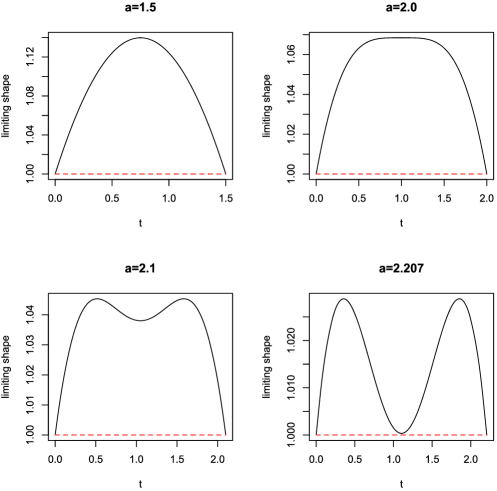
Figure 1: Limiting shapes $x_{a}$ for the stationary Gaussian process with covariance function $R_{\mathbf{X}}(t)=\exp(-t^{2}/2)$ when Proposition 5.3 applies.

The plots of Figure 1 indicate that as $a$ approaches a critical value (approximately $2.2079$ in this case), the limiting curve $x_{a}$ “attempts” to cross the level 1 at the midpoint of $[0,a]$. Equivalently, the normalized process $u^{-1}\mathbf{X}$ attempts to drop below level 1 at that point and so, speaking heuristically, it has to be “supported” at the midpoint $t=a/2$. The interpretation of Theorem 4.1 in Remark 4.2 calls for adding a mass to the measure $\mu^{(1)}$ for the critical value of $a$ at the midpoint of the interval. The next result shows that, in certain cases, this is indeed the optimal thing to do.

Proposition 5.5

Let $\mathbf{X}$ be a stationary continuous Gaussian process. Suppose that, for some $a>0$,

$$R_{\mathbf{X}}(0)+R_{\mathbf{X}}(a)>2R_{\mathbf{X}}(a/2),$$ (47)

and let

$$\varepsilon_{a}=\frac{R_{\mathbf{X}}(0)+R_{\mathbf{X}}(a)-2R_{\mathbf{X}}(a/2)}{3R_{\mathbf{X}}(0)+R_{\mathbf{X}}(a)-4R_{\mathbf{X}}(a/2)}\in(0,1].$$ (48)

Suppose that for all $0\leq t\leq a/2$,

$$R_{\mathbf{X}}(t)+R_{\mathbf{X}}(a-t)-R_{\mathbf{X}}(0)-R_{\mathbf{X}}(a)$$

$$\qquad\geq\varepsilon_{a}\bigl{[}R_{\mathbf{X}}(t)+R_{\mathbf{X}}(a-t)-R_{\mathbf{X}}(0)-R_{\mathbf{X}}(a)$$ (49)

$$\hskip 78.0pt{}-2\bigl{(}R_{\mathbf{X}}(a/2-t)-R_{\mathbf{X}}(a/2)\bigr{)}\bigr{]}.$$

Then a measure in $\mathcal{W}_{a}$ is given by

$$\mu^{(2)}\stackrel{{\scriptstyle\Delta}}{{=}}\frac{1-\varepsilon_{a}}{2}\delta_{0}+\frac{1-\varepsilon_{a}}{2}\delta_{1}+\varepsilon_{a}\delta_{1/2}.$$ (50)

Furthermore,

$$C_{\mathbf{X}}(a) = \frac{3R_{\mathbf{X}}(0)+R_{\mathbf{X}}(a)-4R_{\mathbf{X}}(a/2)}{R_{\mathbf{X}}(0)^{2}+R_{\mathbf{X}}(0)R_{\mathbf{X}}(a)-2R_{\mathbf{X}}(a/2)^{2}},$$ (51)

$$h_{a}(x) = C_{\mathbf{X}}(a)\biggl{[}\frac{1-\varepsilon_{a}}{2}\bigl{(}1+e^{iax}\bigr{)}+\varepsilon_{a}e^{iax/2}\biggr{]}$$ (52)

for $F_{\mathbf{X}}$-almost all $-\infty<x<\infty$, and

$$x_{a}(t)=C_{\mathbf{X}}(a)\biggl{[}\frac{1-\varepsilon_{a}}{2}\bigl{(}R_{\mathbf{X}}(t)+R_{\mathbf{X}}(a-t)\bigr{)}+\varepsilon_{a}R_{\mathbf{X}}\bigl{(}|t-a/2|\bigr{)}\biggr{]},$$ (53)

$0\leq t\leq a$.

The proof is identical to that of Proposition 5.3 once we observe that, under (47), $\mu^{(2)}$ is a legitimate probability measure.

The plots of Figure 2 show the limiting shape $x_{a}$ for the stationary Gaussian process with covariance function $R_{\mathbf{X}}(t)=\exp(-t^{2}/2)$, for a range of $a$ for which Proposition 5.5 applies. In this case the range of $a$ is, approximately, between $2.2079$ and $3.9283$. See Example 6.1 for more details.

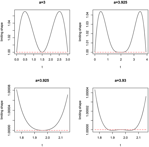
Figure 2: Limiting shapes for $R_{\mathbf{X}}(t)=\exp(-t^{2}/2)$ when Proposition 5.5 applies (the top row). The left plot in the bottom row is a blowup of the right plot in the top row. The right plot in the bottom row shows how the constraints are violated soon after the upper critical value of $a$.

6 Specific covariance functions

In the previous section we saw some general results for one-dimensional processes, with some illustrative figures for what happens in the case of a Gaussian covariance function. In this section we look more carefully at this case, and also look at what can be said for an exponential covariance.

Example 6.1.

Consider the centered stationary Gaussian process with the Gaussian covariance function

$$R(t)=e^{-t^{2}/2},\qquad t\in\mathbb{R}.$$ (54)

For this process the spectral measure has a Gaussian spectral density which is of full support in $\mathbb{R}$. In particular, for every $a>0$ there is a unique (symmetric) measure of minimal energy. Furthermore, the second spectral moment is finite, so that, according to Remark 5.4, for $a>0$ sufficiently small this process satisfies the conditions of Proposition 5.3. To find the range of $a$ for which this happens, note that conditions (41) become, in this case,

$$e^{-t^{2}/2}+e^{-(a-t)^{2}/2}\geq 1+e^{-a^{2}/2},\qquad 0\leq t\leq a.$$ (55)

Since the function

$$g(t)=e^{-t^{2}/2}+e^{-(a-t)^{2}/2},\qquad 0\leq t\leq a,$$

is concave if $0\leq a\leq 2$, and has a unique local minimum, at $t=a/2$, when $a>2$, it is only necessary to check (55) at the midpoint $t=a/2$. At that point the condition becomes

$$\psi(a)=2e^{-a^{2}/8}-1-e^{-a^{2}/2}\geq 0.$$

The function $\psi$ crosses 0 at $a_{1}\approx 2.2079$, which is the limit of the validity of the situation of Proposition 5.3 in this case. The plots of Figure 1 show the limiting shape $x_{a}$ for this process in the situation of Proposition 5.3.

Somewhat longer (and numerical) calculations show that the conditions of Proposition 5.5 hold for the process with the covariance function (54) for an interval of values of $a$ after the conditions of Proposition 5.3 break down. The conditions of Proposition 5.5 continue to hold until the second derivative at the midpoint $t=a/2$ of the limiting function in (53) becomes negative (so that the function takes values smaller than 1 in a neighborhood of the midpoint). To find when this happens, we solve the equation

$$\frac{1-\varepsilon_{a}}{2}\bigl{(}R_{\mathbf{X}}^{\prime\prime}(t)+R_{\mathbf{X}}^{\prime\prime}(a-t)\bigr{)}+\varepsilon_{a}R_{\mathbf{X}}^{\prime\prime}\bigl{(}|t-a/2|\bigr{)}=0$$

at $t=a/2$. The resulting equation

$$(1-\varepsilon_{a})\bigl{(}a^{2}/4-1\bigr{)}e^{-a^{2}/8}-\varepsilon_{a}=0$$

has the solution $a_{2}\approx 3.9283$, which is the limit of the validity of the situation of Proposition 5.5 in this case. The plots of Figure 2 shed some light on the above discussion. This discussion indicates, and calculations confirm, that, in the next regime, the mass in the middle for the optimal measure splits into two parts that start to move away from the center. Heuristically, this is needed “to support” the trajectory that, otherwise, would “dip” below 1 outside of the midpoint.

These calculations rapidly become complicated. They seem to indicate that the next regime continues to hold until around $a_{3}\approx 5.4508$. In this regime the optimal measure takes the form

$$\mu^{(3)}\stackrel{{\scriptstyle\Delta}}{{=}}\frac{1-\varepsilon_{a}}{2}\delta_{0}+\frac{1-\varepsilon_{a}}{2}\delta_{1}+\frac{\varepsilon_{a}}{2}\delta_{1/2-d_{a}}+\frac{\varepsilon_{a}}{2}\delta_{1/2+d_{a}},$$ (56)

where $d_{a}$ is the distance of two internal masses from the midpoint. When $a=4.5$, $\varepsilon_{4.5}=0.36632$ and $d_{4.5}=0.12285$, so that the internal atoms are at $0.37715$ and $0.62285$, and the rest of the support is concentrated at the endpoints of the interval with probabilities $0.31684$. Figure 3 shows the limiting shape $x_{4.5}$.

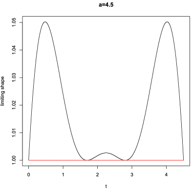
Figure 3: The limiting shape in the case $a=4.5$ for $R_{\mathbf{X}}(t)=\exp(-t^{2}/2).$

It would be nice to understand all regimes, but we do not yet know how to find a general structure. On the other hand, Section 7 gives asymptotic results for $a\to\infty$.

Finally, Figure 4 shows the growth of the exponent $C_{\mathbf{X}}(a)$ with $a$ for as long as either Proposition 5.3 or Proposition 5.5 applies.

Figure 4: The exponent $C_{\mathbf{X}}(a)$ as a function of $a$ for $R_{\mathbf{X}}(t)=\exp(-t^{2}/2)$.

The next example shows a situation very different from that of Example 6.1.

Example 6.2.

Consider an Ornstein–Uhlenbeck process, that is, a centered stationary Gaussian process with the covariance function

$$R(t)=e^{-|t|},\qquad t\in\mathbb{R}.$$ (57)

For this process the spectral measure has a Cauchy spectral density, so it is also of full support in $\mathbb{R}$. Therefore, for every $a>0$ there is a unique (symmetric) measure of minimal energy. In this case, however, even the first spectral moment is infinite. The covariance function is actually convex on the positive half-line so, in particular, the conditions of Proposition 5.3 fail for all $a>0$. In fact, it is elementary to check that for the probability measure

$$\mu=\frac{1}{a+2}\delta_{0}+\frac{1}{a+2}\delta_{1}+\frac{a}{a+2}\lambda$$ (58)

[where $\lambda$ is the Lebesgue measure on $(0,1)$], the integrals

$$\int_{0}^{1}R_{\mathbf{X}}\bigl{(}a(u-v)\bigr{)}\mu(du),\qquad 0\leq v\leq 1,$$

have a constant value, equal to $2/(a+2)$. Therefore, the measure $\mu$ in (58) is the measure of minimal energy, and $C_{\mathbf{X}}(a)=(a+2)/2$ for all $a>0$.

By Theorem 5.1 we conclude that the limiting function $x_{a}$ is equal to 1 almost everywhere in $[0,a]$ with respect to the Lebesgue measure. Since $x_{a}$ is continuous, it is identically equal to 1 on $[0,a]$.

Examples 6.1 and 6.2 demonstrate a number of the ways a stationary Gaussian process “prefers,” in the large deviations sense, to stay above a high level over an interval. The process of Example 6.1 with covariance function (54) is smooth; the most likely way for it to stay above a level is to force it to be “slightly” above that level at a properly chosen finite set of time points; after that it is “held” above the level at the rest of the interval $[0,a]$ by the correlations of the process. The optimal configuration of the finite set of points depends on the length of the interval $[0,a]$, and it appears to undergo phase transitions at certain critical interval lengths. The complete picture of this “dynamical system” of finite sets remains unclear. On the other hand, the Ornstein–Uhlenbeck process of Example 6.2 is continuous, but not smooth. In fact, it behaves locally like a Brownian motion. Therefore, “holding” it “slightly” above a level at a discrete point does not help, since it “wants” immediately to go below that level. This explains the nature of the optimal measure $\mu$ in (58), and this nature stays the same no matter how short or long the interval $[0,a]$ is. In particular, phase transitions do not happen for this process.

It remains to be investigated whether other types of behavior are possible, and under what exact conditions on the Gaussian process each type of behavior occurs. It is also likely that minimal energy measures in $\mathcal{W}_{a}$ carry additional information, describing how “slightly” above the level $u$ a Gaussian process is most likely to be, given that it is above that level along the interval. The exact nature of this information also remains to be investigated.

7 Asymptotics for long intervals

In this section we investigate the asymptotics of the exponent $C_{\mathbf{X}}(a)$ for large $a$. We start with a result showing that, for certain short memory stationary Gaussian processes, the exponent $C_{\mathbf{X}}(a)$ grows linearly with $a$ over long intervals. Furthermore, the energy of the uniform distribution $\lambda$ on $[0,1]$ becomes, asymptotically, minimal.

Theorem 7.1

Let $\mathbf{X}$ be a stationary continuous Gaussian process. Assume that $R_{\mathbf{X}}$ is positive, and satisfies the following condition:

$$\int_{0}^{\infty}R(t)\,dt<\infty.$$ (59)

Then, with $\lambda$ denoting the uniform probability measure on $[0,1]$,

$$\lim_{a\to\infty}\frac{1}{a}C_{\mathbf{X}}(a) = \biggl{(}\lim_{a\to\infty}a\int_{0}^{1}\int_{0}^{1}R_{\mathbf{X}}\bigl{(}a(u-v)\bigr{)}\lambda(du)\lambda(dv)\biggr{)}^{-1}$$

$$= \frac{1}{2\int_{0}^{\infty}R(t)\,dt}.$$

By Theorem 5.1, the statement of the present theorem is equivalent to the following pair of claims:

$$\lim_{a\to\infty}a\int_{0}^{1}\int_{0}^{1}R_{\mathbf{X}}\bigl{(}a(u-v)\bigr{)}\lambda(du)\lambda(dv)=2\int_{0}^{\infty}R(t)\,dt$$ (61)

and

$$\qquad\liminf_{a\to\infty}a\min_{\mu\in M_{1}^{+}([0,1])}\int_{0}^{1}\int_{0}^{1}R_{\mathbf{X}}\bigl{(}a(u-v)\bigr{)}\mu(du)\mu(dv)\geq 2\int_{0}^{\infty}R(t)\,dt.$$ (62)

Since

$$\int_{0}^{1}\int_{0}^{1}R_{\mathbf{X}}\bigl{(}a(u-v)\bigr{)}\lambda(du)\lambda(dv)$$

$$\qquad=\frac{1}{a}\int_{0}^{1}\biggl{[}\int_{0}^{av}R(t)\,dt+\int_{0}^{a(1-v)}R(t)\,dt\biggr{]}\,dv,$$

(61) immediately follows from (59) and the bounded convergence theorem. Therefore, it only remains to prove (62). Suppose that, to the contrary, (62) fails, and choose a sequence $a_{n}\to\infty$ such that

$$\lim_{n\to\infty}a_{n}\min_{\mu\in M_{1}^{+}([0,1])}\int_{0}^{1}\int_{0}^{1}R_{\mathbf{X}}\bigl{(}a_{n}(u-v)\bigr{)}\mu(du)\mu(dv)<2\int_{0}^{\infty}R(t)\,dt.$$

For each $n$ choose a symmetric $\mu_{a_{n}}\in{\mathcal{W}}_{a_{n}}$, so that

$$\lim_{n\to\infty}a_{n}\int_{0}^{1}\int_{0}^{1}R_{\mathbf{X}}\bigl{(}a_{n}(u-v)\bigr{)}\mu_{a_{n}}(du)\mu_{a_{n}}(dv)<2\int_{0}^{\infty}R(t)\,dt.$$ (63)

We claim that, for every $\gamma>0$,

$$\lim_{n\to\infty}\mu_{a_{n}}\bigl{(}\bigl{[}0,\gamma a_{n}^{-1}\bigr{]}\bigr{)}=0.$$ (64)

Indeed, by the positivity of $R_{\mathbf{X}}$, for any $\gamma>0$,

$$\int_{0}^{1}\int_{0}^{1}R_{\mathbf{X}}\bigl{(}a_{n}(u-v)\bigr{)}\mu_{a_{n}}(du)\mu_{a_{n}}(dv)$$

$$\qquad\geq\int_{0}^{\gamma a_{n}^{-1}}\int_{0}^{\gamma a_{n}^{-1}}R_{\mathbf{X}}\bigl{(}a_{n}(u-v)\bigr{)}\mu_{a_{n}}(du)\mu_{a_{n}}(dv)$$

$$\qquad\geq\bigl{\{}\mu_{a_{n}}\bigl{(}\bigl{[}0,\gamma a_{n}^{-1}\bigr{]}\bigr{)}\bigr{\}}^{2}\inf_{0\leq t\leq\gamma}R(t),$$

so that (63) necessitates (64). Next, define a sequence of signed measures on $[0,1]$ by $\hat{\mu}_{n}=\mu_{a_{n}}-\lambda$. Note that

$$\hat{\mu}_{n}\bigl{(}[0,1]\bigr{)}=0\qquad\mbox{for each $n$.}$$ (65)

By the nonnegative definiteness of $R_{\mathbf{X}}$,

$$\int_{0}^{1}\int_{0}^{1}R_{\mathbf{X}}\bigl{(}a_{n}(u-v)\bigr{)}\mu_{a_{n}}(du)\mu_{a_{n}}(dv)$$

$$\qquad=\int_{0}^{1}\int_{0}^{1}R_{\mathbf{X}}\bigl{(}a_{n}(u-v)\bigr{)}\lambda(du)\lambda(dv)+\int_{0}^{1}\int_{0}^{1}R_{\mathbf{X}}\bigl{(}a_{n}(u-v)\bigr{)}\hat{\mu}_{n}(du)\hat{\mu}_{n}(dv)$$

$$\qquad\quad{}+2\int_{0}^{1}\int_{0}^{1}R_{\mathbf{X}}\bigl{(}a_{n}(u-v)\bigr{)}\lambda(du)\hat{\mu}_{n}(dv)$$

$$\qquad\geq\int_{0}^{1}\int_{0}^{1}R_{\mathbf{X}}\bigl{(}a_{n}(u-v)\bigr{)}\lambda(du)\lambda(dv)$$

$$\qquad\quad{}+2\int_{0}^{1}\int_{0}^{1}R_{\mathbf{X}}\bigl{(}a_{n}(u-v)\bigr{)}\lambda(du)\hat{\mu}_{n}(dv).$$

We will show that

$$\lim_{n\to\infty}a_{n}\int_{0}^{1}\int_{0}^{1}R_{\mathbf{X}}\bigl{(}a_{n}(u-v)\bigr{)}\lambda(du)\hat{\mu}_{n}(dv)=0.$$ (66)

Together with (61) this will provide the necessary contradiction to (63). Let $\gamma>0$. Write the integral in (66) as

$$\int_{\gamma a_{n}^{-1}}^{1-\gamma a_{n}^{-1}}\biggl{[}\int_{0}^{1}R_{\mathbf{X}}\bigl{(}a_{n}(u-v)\bigr{)}\,du\biggr{]}\hat{\mu}_{n}(dv)$$

$$\quad{}+2\int_{0}^{\gamma a_{n}^{-1}}\biggl{[}\int_{0}^{1}R_{\mathbf{X}}\bigl{(}a_{n}(u-v)\bigr{)}\,du\biggr{]}\hat{\mu}_{n}(dv)$$

$$\qquad\stackrel{{\scriptstyle\Delta}}{{=}}J_{n}^{(1)}+2J_{n}^{(2)}.$$

Observe that

$$\bigl{|}J_{n}^{(2)}\bigr{|} = \frac{1}{a_{n}}\biggl{|}\int_{0}^{\gamma a_{n}^{-1}}\biggl{[}\int_{0}^{a_{n}v}R_{\mathbf{X}}(t)\,dt+\int_{0}^{a_{n}(1-v)}R_{\mathbf{X}}(t)\,dt\biggr{]}\hat{\mu}_{n}(dv)\biggr{|}$$

$$\leq \frac{2\int_{0}^{\infty}R_{\mathbf{X}}(t)\,dt}{a_{n}}\|\hat{\mu}_{n}\|\bigl{(}\bigl{[}0,\gamma a_{n}^{-1}\bigr{]}\bigr{)},$$

so that by (64) we obtain

$$\lim_{n\to\infty}a_{n}J_{n}^{(2)}=0$$ (67)

for every $\gamma>0$. Next, we write

$$J_{n}^{(1)} = \frac{1}{a_{n}}\int_{\gamma a_{n}^{-1}}^{1-\gamma a_{n}^{-1}}\biggl{[}\int_{0}^{a_{n}v}R_{\mathbf{X}}(t)\,dt+\int_{0}^{a_{n}(1-v)}R_{\mathbf{X}}(t)\,dt\biggr{]}\hat{\mu}_{n}(dv)$$

$$= \frac{2\int_{0}^{\infty}R_{\mathbf{X}}(t)\,dt}{a_{n}}\hat{\mu}_{n}\bigl{(}\bigl{[}\gamma a_{n}^{-1},1-\gamma a_{n}^{-1}\bigr{]}\bigr{)}$$

$${}-\frac{1}{a_{n}}\int_{\gamma a_{n}^{-1}}^{1-\gamma a_{n}^{-1}}\biggl{[}\int_{a_{n}v}^{\infty}R_{\mathbf{X}}(t)\,dt+\int_{a_{n}(1-v)}^{\infty}R_{\mathbf{X}}(t)\,dt\biggr{]}\hat{\mu}_{n}(dv)$$

$$\stackrel{{\scriptstyle\Delta}}{{=}} J_{n}^{(11)}-J_{n}^{(12)}.$$

It follows from (65) that

$$\qquad\bigl{|}a_{n}J_{n}^{(11)}\bigr{|}=2\int_{0}^{\infty}R_{\mathbf{X}}(t)\,dt\bigl{|}\hat{\mu}_{n}\bigl{(}\bigl{[}0,\gamma a_{n}^{-1}\bigr{]}\bigr{)}+\hat{\mu}_{n}\bigl{(}\bigl{[}1-\gamma a_{n}^{-1},1\bigr{]}\bigr{)}\bigr{|}\to 0$$ (68)

as $n\to\infty$, by (64). Finally,

$$\bigl{|}a_{n}J_{n}^{(12)}\bigr{|}\leq 4\int_{\gamma}^{\infty}R_{\mathbf{X}}(t)\,dt,$$ (69)

and we obtain by (67), (68) and (69) that

$$\limsup_{n\to\infty}a_{n}\biggl{|}\int_{0}^{1}\int_{0}^{1}R_{\mathbf{X}}\bigl{(}a_{n}(u-v)\bigr{)}\lambda(du)\hat{\mu}_{n}(dv)\biggr{|}\leq 4\int_{\gamma}^{\infty}R_{\mathbf{X}}(t)\,dt.$$

Letting $\gamma\to\infty$ proves (66) and, hence, completes the proof of the theorem.

The next theorem is the counterpart of Theorem 7.1 for certain long memory stationary Gaussian processes. In this case, the uniform distribution on $[0,1]$ is no longer, asymptotically, optimal. We will assume that the covariance function of the process is regularly varying at infinity:

$$R_{\mathbf{X}}(t)=\frac{L(t)}{|t|^{\beta}},\qquad 0<\beta<1,$$ (70)

where $L$ is slowly varying at infinity. Before stating the theorem, we introduce new notation.

Consider the minimization problem

$$\min_{\mu\in M_{1}^{+}([0,1])}\int_{0}^{1}\int_{0}^{1}\frac{\mu(du)\mu(dv)}{|u-v|^{\beta}},\qquad 0<\beta<1.$$ (71)

This is a minimization problem of the same nature as in (37) with $a=0,b=1$, and the covariance function $R_{\mathbf{X}}$ replaced by the Riesz kernel $K_{\beta}(u,v)=|u-v|^{-\beta}$, $u,v\in[0,1]$. The general theory of energy of measures in fuglede1960 applies to the Riesz kernel. In particular, the minimum in (71) is well defined, is finite and positive. Let ${\mathcal{W}}_{\beta}$ be the set of measures in $M_{1}^{+}([0,1])$ of minimal energy with respect to the Riesz kernel. Note that the uniform measure $\lambda\notin{\mathcal{W}}_{\beta}$ since it does not satisfy the optimality conditions in Theorem 2.4 in fuglede1960 .

Theorem 7.2

Let $\mathbf{X}$ be a continuous stationary Gaussian process. Assume that $R_{\mathbf{X}}$ is positive and satisfies assumption (70) of regular variation. Then for any $\mu_{\beta}\in{\mathcal{W}}_{\beta}$,

$$\lim_{a\to\infty}R_{\mathbf{X}}(a)\mathcal{C}_{\mathbf{X}}(\mathbf{a})=\biggl{(}\int_{0}^{1}\int_{0}^{1}\frac{\mu_{\beta}(du)\mu_{\beta}(dv)}{|u-v|^{\beta}}\biggr{)}^{-1}.$$ (72)

Suppose first that there is a sequence $a_{n}\uparrow\infty$ such that

$$\lim_{n\to\infty}\frac{1}{R_{\mathbf{X}}(a_{n})}\min_{\mu\in M_{1}^{+}([0,1])}\int_{0}^{1}\int_{0}^{1}R_{\mathbf{X}}\bigl{(}a_{n}(u-v)\bigr{)}\mu(du)\mu(dv)$$

(73)

$$\qquad<\int_{0}^{1}\int_{0}^{1}\frac{\mu_{\beta}(du)\mu_{\beta}(dv)}{|u-v|^{\beta}}.$$

For each $n$ choose $\mu_{n}\in{\mathcal{W}}_{a_{n}}$, let $n_{k}\uparrow\infty$ be a subsequence such that $\mu_{n_{k}}\Rightarrow\hat{\mu}$ weakly as $k\to\infty$ for some $\hat{\mu}\in M_{1}^{+}([0,1])$. By Fatou’s lemma and the regular variation of $R_{\mathbf{X}}$,

$$\liminf_{k\to\infty}\frac{1}{R_{\mathbf{X}}(a_{n_{k}})}\int_{0}^{1}\int_{0}^{1}R_{\mathbf{X}}\bigl{(}a_{n_{k}}(u-v)\bigr{)}\mu_{n_{k}}(du)\mu_{n_{k}}(dv)$$

$$\qquad\geq\int_{0}^{1}\int_{0}^{1}\frac{\hat{\mu}(du)\hat{\mu}(dv)}{|u-v|^{\beta}}\geq\int_{0}^{1}\int_{0}^{1}\frac{\mu_{\beta}(du)\mu_{\beta}(dv)}{|u-v|^{\beta}},$$

since $\mu_{\beta}$ has the smallest energy with respect to the Riesz kernel. This contradicts (7), thus proving that

$$\liminf_{a\to\infty}\frac{1}{R_{\mathbf{X}}(a)}\min_{\mu\in M_{1}^{+}([0,1])}\int_{0}^{1}\int_{0}^{1}R_{\mathbf{X}}\bigl{(}a(u-v)\bigr{)}\mu(du)\mu(dv)$$

(74)

$$\qquad\geq\int_{0}^{1}\int_{0}^{1}\frac{\mu_{\beta}(du)\mu_{\beta}(dv)}{|u-v|^{\beta}}.$$

In order to finish the proof, we need to establish a matching upper limit bound.

To this end, let $\theta>0$ be a small number. We define a probability measure $\nu_{\theta}\in M_{1}^{+}([0,1])$ by convolving $\mu_{\beta}$ with the uniform distribution on $[0,\theta]$ and rescaling the resulting convolution back to the unit interval. More explicitly, if $X$ and $U$ are independent random variables, whose laws are $\mu_{\beta}$ and $\lambda$, respectively, then $\nu_{\theta}$ is the law of $(X+\theta U)/(1+\theta)$. Note that

$$\nu_{\theta}\ll\lambda\qquad\mbox{and}\qquad\frac{d\nu_{\theta}}{d\lambda}\leq\frac{1+\theta}{\theta}\qquad\mbox{a.e. on $[0,1]$.}$$ (75)

Given $0<\varepsilon<1-\beta$, by Potter’s bounds (see, e.g., Proposition 0.8 in resnick1987 ), there is $t_{0}>0$ sufficiently large to ensure

$$\frac{R_{\mathbf{X}}(tx)}{R_{\mathbf{X}}(t)}>(1-\varepsilon)x^{-\beta-\varepsilon}$$

for all $t\geq t_{0}$ and $x\geq 1$. We have

$$\min_{\mu\in M_{1}^{+}([0,1])}\int_{0}^{1}\int_{0}^{1}R_{\mathbf{X}}\bigl{(}a(u-v)\bigr{)}\mu(du)\mu(dv)$$

$$\qquad\leq\int_{0}^{1}\int_{0}^{1}R_{\mathbf{X}}\bigl{(}a(u-v)\bigr{)}\nu_{\theta}(du)\nu_{\theta}(dv)$$

$$\qquad=\int_{0}^{1}\int_{0}^{1}\mathbf{1}\bigl{(}|u-v|\leq t_{0}/a\bigr{)}R_{\mathbf{X}}\bigl{(}a(u-v)\bigr{)}\nu_{\theta}(du)\nu_{\theta}(dv)$$

$$\qquad\quad{}+\int_{0}^{1}\int_{0}^{1}\mathbf{1}\bigl{(}|u-v|>t_{0}/a\bigr{)}R_{\mathbf{X}}\bigl{(}a(u-v)\bigr{)}\nu_{\theta}(du)\nu_{\theta}(dv)$$

$$\qquad\stackrel{{\scriptstyle\Delta}}{{=}}I_{1}(a)+I_{2}(a).$$

By the definition of $t_{0}$,

$$\mathbf{1}\bigl{(}|u-v|>t_{0}/a\bigr{)}\frac{R_{\mathbf{X}}(a(u-v))}{R_{\mathbf{X}}(a)}\leq\frac{1}{1+\varepsilon}|u-v|^{-(\beta+\varepsilon)},$$

so that by the dominated convergence theorem we have

$$\lim_{a\to\infty}\frac{1}{R_{\mathbf{X}}(a)}I_{2}(a)=\int_{0}^{1}\int_{0}^{1}\frac{\nu_{\theta}(du)\nu_{\theta}(dv)}{|u-v|^{\beta}}.$$

On the other hand, by (75),

$$I_{1}(a)\leq R_{\mathbf{X}}(0)\frac{2t_{0}}{a}\frac{1+\theta}{\theta}=o\bigl{(}R_{\mathbf{X}}(a)\bigr{)}$$

as $a\to\infty$. We conclude that

$$\limsup_{a\to\infty}\frac{1}{R_{\mathbf{X}}(a)}\min_{\mu\in M_{1}^{+}([0,1])}\int_{0}^{1}\int_{0}^{1}R_{\mathbf{X}}\bigl{(}a(u-v)\bigr{)}\mu(du)\mu(dv)$$

$$\qquad\leq\int_{0}^{1}\int_{0}^{1}\frac{\nu_{\theta}(du)\nu_{\theta}(dv)}{|u-v|^{\beta}}.$$

Once we show that

$$\lim_{\theta\to 0}\int_{0}^{1}\int_{0}^{1}\frac{\nu_{\theta}(du)\nu_{\theta}(dv)}{|u-v|^{\beta}}=\int_{0}^{1}\int_{0}^{1}\frac{\mu_{\beta}(du)\mu_{\beta}(dv)}{|u-v|^{\beta}},$$ (76)

we will have established an upper bound matching (7). This will complete the proof of the theorem. Recall that (76) is equivalent to

$$\lim_{\theta\to 0}E\bigl{|}X_{1}-X_{2}+\theta(U_{1}-U_{2})\bigr{|}^{-\beta}=E|X_{1}-X_{2}|^{-\beta},$$

where $X_{1},X_{2},U_{1},U_{2}$ are independent random variables, $X_{1}$ and $X_{2}$ with the law $\mu_{\beta}$, while $U_{1}$ and $U_{2}$ are uniformly distributed on $[0,1]$. This, however, follows by the dominated convergence theorem and the following fact, that can be checked by elementary calculations: there is $r_{\beta}\in(0,\infty)$ such that for any $0<b<1$ and $0<\theta<1$,

$$E\bigl{|}b+\theta(U_{1}-U_{2})\bigr{|}^{-\beta}\leq r_{\beta}b^{-\beta}.$$

Remark 7.3.

It follows from Proposition A.3 in khoshnevisanxiaozhong2003 that the energy of the measure $\mu_{\beta}$ with respect to the Riesz kernel cannot be smaller than one half of the energy of the uniform measure. Hence,

$$\lim_{a\to\infty}R_{\mathbf{X}}(a)\mathcal{C}_{\mathbf{X}}(\mathbf{a})\in\bigl{(}(1-\beta)(2-\beta)/2,(1-\beta)(2-\beta)\bigr{)}.$$

8 The multidimensional case

Our understanding of the one-dimensional case described in the previous three sections, while incomplete, is nevertheless quite significant. In contrast, there is much less we can say about the multivariate problem of Section 3. The problem lies, in part, in the nonconvexity of the feasible set in (9) which leads, in turn, to the “max-min” problem in Theorem 3.2.

The following proposition is a multivariate version of Proposition 41. Note that stationarity of the random field is not required.

Proposition 8.1

Let $\mathbf{X}=(X(\mathbf{t}),\mathbf{t}\in T)$ be a continuous Gaussian random field on a compact set $T\subset\mathbb{R}^{d}$, and suppose that $\mathbf{a},\mathbf{b}$ are in $T$. Suppose that there is a path $\xi_{0}$ in $T$ connecting $\mathbf{a}$ and $\mathbf{b}$ such that

$$\qquad R_{\mathbf{X}}\bigl{(}\mathbf{a},\xi_{0}(u)\bigr{)}+R_{\mathbf{X}}\bigl{(}\xi_{0}(u),\mathbf{b}\bigr{)}\geq\frac{R_{\mathbf{X}}(\mathbf{a},\mathbf{a})+2R_{\mathbf{X}}(\mathbf{a},\mathbf{b})+R_{\mathbf{X}}(\mathbf{b},\mathbf{b})}{2}>0$$ (77)

for all $0\leq u\leq 1$. Then the supremum in (3.2) is achieved on the path $\xi_{0}$ and

$$\mathcal{C}_{\mathbf{X}}(\mathbf{a},\mathbf{b})=\frac{4}{R_{\mathbf{X}}(\mathbf{a},\mathbf{a})+2R_{\mathbf{X}}(\mathbf{a},\mathbf{b})+R_{\mathbf{X}}(\mathbf{b},\mathbf{b})}.$$ (78)

Remark 8.2.

Using $u=0$ and $u=1$ in (77) shows that conditions of Proposition 8.1 cannot be satisfied unless $R_{\mathbf{X}}(\mathbf{a},\mathbf{a})=R_{\mathbf{X}}(\mathbf{b},\mathbf{b})$. Correspondingly, we can restate (78) as

$$\mathcal{C}_{\mathbf{X}}(\mathbf{a},\mathbf{b})=\frac{2}{R_{\mathbf{X}}(\mathbf{a},\mathbf{a})+R_{\mathbf{X}}(\mathbf{a},\mathbf{b})}.$$

Recall (46), which shows that this implies the logarithmic equivalence of the probabilities of $\mathbf{X}$ being above the level $u$ along a curve or at its endpoints.

Proof of Proposition 8.1 Consider the fixed path $\xi_{0}$. The assumption (77) shows that the measure

$$\mu_{0}=\tfrac 12\delta_{a}+\tfrac 12\delta_{b}$$

satisfies conditions (4.3) and, hence, is in ${\mathcal{W}}_{\xi_{0}}$ by Theorem 4.3. Therefore,

$$\min_{\mu\in M_{1}^{+}([0,1])}\int_{0}^{1}\int_{0}^{1}R_{\mathbf{X}}\bigl{(}\xi_{0}(u),\xi_{0}(v)\bigr{)}\mu(du)\mu(dv)$$

$$\qquad=\int_{0}^{1}\int_{0}^{1}R_{\mathbf{X}}\bigl{(}\xi_{0}(u),\xi_{0}(v)\bigr{)}\mu_{0}(du)\mu_{0}(dv)$$

$$\qquad=\frac{R_{\mathbf{X}}(\mathbf{a},\mathbf{a})+2R_{\mathbf{X}}(\mathbf{a},\mathbf{b})+R_{\mathbf{X}}(\mathbf{b},\mathbf{b})}{4}.$$

On the other hand, for any other path in $T$ connecting $\mathbf{a}$ and $\mathbf{b}$,

$$\min_{\mu\in M_{1}^{+}([0,1])}\int_{0}^{1}\int_{0}^{1}R_{\mathbf{X}}\bigl{(}\xi(u),\xi(v)\bigr{)}\mu(du)\mu(dv)$$

$$\qquad\leq\int_{0}^{1}\int_{0}^{1}R_{\mathbf{X}}\bigl{(}\xi(u),\xi(v)\bigr{)}\mu_{0}(du)\mu_{0}(dv)$$

$$\qquad=\frac{R_{\mathbf{X}}(\mathbf{a},\mathbf{a})+2R_{\mathbf{X}}(\mathbf{a},\mathbf{b})+R_{\mathbf{X}}(\mathbf{b},\mathbf{b})}{4}.$$

Therefore, the supremum in (3.2) is achieved on the path $\xi_{0}$, and (78) follows by Theorem 3.2.

Even for the most common Gaussian random fields, the assumptions of Proposition 8.1 may be satisfied on some path but not on the straight line connecting the two points. In that case, the straight line, clearly, fails to be optimal.

Example 8.3.

Consider a Brownian sheet in $d\geq 2$ dimensions. This is the continuous centered Gaussian random field $\mathbf{X}$ on $[0,\infty)^{d}$ with covariance function

$$R_{\mathbf{X}}(\mathbf{s},\mathbf{t})=\prod_{j=1}^{d}\min(s_{j},t_{j}),\qquad\mathbf{s},\mathbf{t}\in[0,\infty)^{d}.$$

We restrict the random field to the hypercube $T=[0,d]^{d}$, and let

$$\mathbf{a}=(1,2,\ldots,d-1,d),\qquad\mathbf{b}=(d,1,2,\ldots,d-1).$$

It is elementary to check that the path

$$\xi_{0}(u)=\cases{\bigl{(}1+d(d-1)u,2,\ldots,d-1,d\bigr{)},&\quad$\mbox{for }0\leq u\leq\displaystyle\frac{1}{d},$\vspace*{2pt}\cr(d,1,\ldots,j-2,2j-1-du,j+1,\ldots,d),&\quad$\mbox{for }\displaystyle\frac{j-1}{d}\leq u\leq\frac{j}{d},$\vspace*{2pt}\cr&\quad$j=2,\ldots,d$,}$$

satisfies (77) and, hence, the supremum in (3.2) is achieved on that path. Therefore, by Proposition 8.1,

$$\mathcal{C}_{\mathbf{X}}(\mathbf{a},\mathbf{b})=\frac{2}{d!+(d-1)!}.$$

On the other hand, if we consider the straight line connecting the points $\mathbf{a}$ and $\mathbf{b}$,

$$\xi(u)=\bigl{(}1+(d-1)u,2-u,3-u,\ldots,d-u\bigr{)},\qquad 0\leq u\leq 1,$$

then the sum in the right-hand side of (77) becomes

$$L(u)=\prod_{j=2}^{d}(j-u)+\bigl{(}1+(d-1)u\bigr{)}(d-1)!,\qquad 0\leq u\leq 1.$$

The function $L$ achieves the value $d!+(d-1)!$ at the endpoints $u=0$ and $u=1$, and is strictly convex if $d\geq 3$. Therefore, it takes values strictly smaller than $d!+(d-1)!$ over $0<u<1$. That is, (77) fails, and the straight line is not optimal. If $d=2$, however, then $L$ is a constant function, condition (77) holds over the straight line path, and the straight line is optimal.

We also note that, if $d=1$, then the Brownian sheet becomes the Brownian motion in one dimension. In that case it is, clearly, impossible to find two positive points $a<b$ in which the process has the same variance, so Proposition 8.1 does not apply. In this case, however, we are in the situation of Theorem 5.1, so if $0<a<b<\infty$, then the measure $\mu=\delta_{a}$ satisfies (5.1) and, hence, is optimal.

The above example notwithstanding, under certain assumptions on the random field, the straight line path between two points turns out to be optimal for the optimization problem (3.2). The next result describes one such situation.

Recall that a random field on $\mathbb{R}^{d}$ is isotropic if its law is invariant under rigid motions of the parameter space. A centered Gaussian random field $\mathbf{X}$ is isotropic if and only if its covariance function is a function of the Euclidian distance between two points. With the usual abuse of notation we will write $R_{\mathbf{X}}(\mathbf{a},\mathbf{b})=R_{\mathbf{X}}(\|\mathbf{b}-\mathbf{a}\|)$, $\mathbf{a},\mathbf{b}\in\mathbb{R}^{d}$.

Proposition 8.4

Let $\mathbf{X}$ be a continuous centered isotropic Gaussian random field, such that the covariance function $R_{\mathbf{X}}$ is nonincreasing. Then for any $\mathbf{a},\mathbf{b}\in\mathbb{R}^{d}$, the straight path connecting the points $\mathbf{a}$ and $\mathbf{b}$ is optimal for the optimization problem (3.2).

We may and will assume, without loss of generality, that $\mathbf{a}=(a,0,\ldots,0)$ and $\mathbf{b}=\mathbf{0}$ for some $a>0$. We start with showing that the supremum over $\xi\in\mathcal{P}(\mathbf{0},\mathbf{a})$ is achieved over paths in

$$\mathcal{P}_{l}=\bigl{\{}\xi\dvtx[0,1]\to\bigl{\{}(x,0,\ldots,0)\dvtx x\geq 0\bigr{\}},\mbox{continuous, }\xi(0)=\mathbf{0},\xi(1)=\mathbf{a}\bigr{\}}.$$

To this end, it is enough to show that for each $\xi\in\mathcal{P}(\mathbf{0},\mathbf{a})$ there is $\hat{\xi}\in\mathcal{P}_{l}$ such that

$$\min_{\mu\in M_{1}^{+}([0,1])}\int_{0}^{1}\int_{0}^{1}R_{\mathbf{X}}\bigl{(}\bigl{\|}\xi(u)-\xi(v)\bigr{\|}\bigr{)}\mu(du)\mu(dv)$$

(79)

$$\qquad\leq\min_{\mu\in M_{1}^{+}([0,1])}\int_{0}^{1}\int_{0}^{1}R_{\mathbf{X}}\bigl{(}\bigl{\|}\hat{\xi}(u)-\hat{\xi}(v)\bigr{\|}\bigr{)}\mu(du)\mu(dv).$$

To see this, define for $\xi\in\mathcal{P}(\mathbf{0},\mathbf{a})$

$$\hat{\xi}(u)=\bigl{(}\bigl{\|}\xi(u)\bigr{\|},0,\ldots,0\bigr{)},\qquad 0\leq u\leq 1.$$

Clearly, $\hat{\xi}\in\mathcal{P}_{l}$, and (8) follows by the monotonicity of $R_{\mathbf{X}}$ and the triangle inequality

$$\bigl{|}\bigl{\|}\xi(u)\bigr{\|}-\bigl{\|}\xi(v)\bigr{\|}\bigr{|}\leq\bigl{\|}\xi(u)-\xi(v)\bigr{\|}.$$

Next, any $\xi\in\mathcal{P}_{l}$ is of the form

$$\xi(u)=\bigl{(}\varphi(u),0,\ldots,0\bigr{)},\qquad 0\leq u\leq 1,$$ (80)

with $\varphi\dvtx[0,1]\to[0,\infty)$ a continuous function, satisfying $\varphi(0)=0$, $\varphi(1)=a$. Defining $\hat{\varphi}(u)=\min(\varphi(u),a)$, $0\leq u\leq 1$, and

$$\hat{\xi}(u)=\bigl{(}\hat{\varphi}(u),0,\ldots,0\bigr{)},\qquad 0\leq u\leq 1,$$

we see that the supremum over paths in $\mathcal{P}_{l}$ is, actually, achieved over paths whose image is exactly the interval $[0,a]$. Finally, for any path $\xi\in\mathcal{P}_{l}$ of the latter type, given in the form (80), define

$$r(v)=\inf\bigl{\{}u\in[0,1]\dvtx\varphi(u)=av\bigr{\}},\qquad 0\leq v\leq 1.$$

Then $r$ is a measurable map from $[0,1]$ to itself, so for any $\mu\in M_{1}^{+}([0,1])$, we can define $\mu_{1}\in M_{1}^{+}([0,1])$ by $\mu_{1}=\mu\circ r^{-1}$. Then

$$\int_{0}^{1}\int_{0}^{1}R_{\mathbf{X}}\bigl{(}\bigl{|}\varphi(u)-\varphi(v)\bigr{|}\bigr{)}\mu_{1}(du)\mu_{1}(dv)$$

$$\qquad=\int_{0}^{1}\int_{0}^{1}R_{\mathbf{X}}\bigl{(}\bigl{|}\varphi\bigl{(}r(u)\bigr{)}-\varphi\bigl{(}r(v)\bigr{)}\bigr{|}\bigr{)}\mu(du)\mu(dv)$$

$$\qquad=\int_{0}^{1}\int_{0}^{1}R_{\mathbf{X}}\bigl{(}a|u-v|\bigr{)}\mu(du)\mu(dv).$$

Therefore,

$$\min_{\mu\in M_{1}^{+}([0,1])}\int_{0}^{1}\int_{0}^{1}R_{\mathbf{X}}\bigl{(}\bigl{\|}\xi(u)-\xi(v)\bigr{\|}\bigr{)}\mu(du)\mu(dv)$$

$$\qquad\leq\min_{\mu\in M_{1}^{+}([0,1])}\int_{0}^{1}\int_{0}^{1}R_{\mathbf{X}}\bigl{(}a|u-v|\bigr{)}\mu(du)\mu(dv),$$

and the statement of the proposition follows.

References

(1){bbook}[mr]
\bauthor\bsnmAdler, \bfnmRobert J.\binitsR. J. and \bauthor\bsnmTaylor, \bfnmJonathan E.\binitsJ. E.
(\byear2007).
\btitleRandom Fields and Geometry.
\bpublisherSpringer, \blocationNew York.
\bidmr=2319516
\bptokimsref
\endbibitem
(2){bbook}[mr]
\bauthor\bsnmAzaïs, \bfnmJean-Marc\binitsJ.-M. and \bauthor\bsnmWschebor, \bfnmMario\binitsM.
(\byear2009).
\btitleLevel Sets and Extrema of Random Processes and Fields.
\bpublisherWiley, \blocationHoboken, NJ.
\biddoi=10.1002/9780470434642, mr=2478201
\bptokimsref
\endbibitem
(3){bbook}[mr]
\bauthor\bsnmDeuschel, \bfnmJean-Dominique\binitsJ.-D. and \bauthor\bsnmStroock, \bfnmDaniel W.\binitsD. W.
(\byear1989).
\btitleLarge Deviations.
\bseriesPure and Applied Mathematics
\bvolume137.
\bpublisherAcademic Press, \blocationBoston, MA.
\bidmr=0997938
\bptokimsref
\endbibitem
(4){barticle}[mr]
\bauthor\bsnmFuglede, \bfnmBent\binitsB.
(\byear1960).
\btitleOn the theory of potentials in locally compact spaces.
\bjournalActa Math.
\bvolume103
\bpages139–215.
\bidissn=0001-5962, mr=0117453
\bptokimsref
\endbibitem
(5){barticle}[mr]
\bauthor\bsnmKhoshnevisan, \bfnmDavar\binitsD.,
\bauthor\bsnmXiao, \bfnmYimin\binitsY. and \bauthor\bsnmZhong, \bfnmYuquan\binitsY.
(\byear2003).
\btitleMeasuring the range of an additive Lévy process.
\bjournalAnn. Probab.
\bvolume31
\bpages1097–1141.
\biddoi=10.1214/aop/1048516547, issn=0091-1798, mr=1964960
\bptokimsref
\endbibitem
(7){bbook}[mr]
\bauthor\bsnmLuenberger, \bfnmDavid G.\binitsD. G.
(\byear1969).
\btitleOptimization by Vector Space Methods.
\bpublisherWiley, \blocationNew York.
\bidmr=0238472
\bptokimsref
\endbibitem
(8){bbook}[mr]
\bauthor\bsnmResnick, \bfnmSidney I.\binitsS. I.
(\byear1987).
\btitleExtreme Values, Regular Variation, and Point Processes.
\bseriesApplied Probability. A Series of the Applied Probability Trust
\bvolume4.
\bpublisherSpringer, \blocationNew York.
\bidmr=0900810
\bptokimsref
\endbibitem
(9){bincollection}[mr]
\bauthor\bparticlevan der \bsnmVaart, \bfnmA. W.\binitsA. W. and \bauthor\bparticlevan \bsnmZanten, \bfnmJ. H.\binitsJ. H.
(\byear2008).
\btitleReproducing kernel Hilbert spaces of Gaussian priors.
In \bbooktitlePushing the Limits of Contemporary Statistics:
Contributions in
Honor of Jayanta K. Ghosh.
\bseriesInst. Math. Stat. Collect.
\bvolume3
\bpages200–222.
\bpublisherIMS, \blocationBeachwood, OH.
\biddoi=10.1214/074921708000000156, mr=2459226
\bptokimsref
\endbibitem