Improved estimation in cumulative link models

Abstract

For the estimation of cumulative link models for ordinal data, the bias-reducing adjusted score equations in Firth (1993) are obtained, whose solution ensures an estimator with smaller asymptotic bias than the maximum likelihood estimator. Their form suggests a parameter-dependent adjustment of the multinomial counts, which, in turn suggests the solution of the adjusted score equations through iterated maximum likelihood fits on adjusted counts, greatly facilitating implementation. Like the maximum likelihood estimator, the reduced-bias estimator is found to respect the invariance properties that make cumulative link models a good choice for the analysis of categorical data. Its additional finiteness and optimal frequentist properties, along with the adequate behaviour of related asymptotic inferential procedures make the reduced-bias estimator attractive as a default choice for practical applications. Furthermore, the proposed estimator enjoys certain shrinkage properties that are defensible from an experimental point of view relating to the nature of ordinal data.
Key words: reduction of bias, adjusted score equations, adjusted counts, shrinkage, ordinal response models.

1 Introduction

In many models with categorical responses the maximum likelihood estimates can be on the boundary of the parameter space with positive probability. For example, Albert and Anderson (1984) derive the conditions that describe when the maximum likelihood estimates are on the boundary in multinomial logistic regression models. While there is no ambiguity in reporting an estimate on the boundary of the parameter space, as is for example an infinite estimate for the parameters of a logistic regression model, estimates on the boundary can (i) cause numerical instabilities to fitting procedures, (ii) lead to misleading output when estimation is based on iterative procedures with a stopping criterion, and more importantly, (iii) cause havoc to asymptotic inferential procedures, and especially to the ones that depend on estimates of the standard error of the estimators (for example, Wald tests and related confidence intervals).

The maximum likelihood estimator in cumulative link models for ordinal data (McCullagh, 1980) also has a positive probability of being on the boundary.

Example 1.1:

As a demonstration consider the example in Christensen (2012a, §7). The data set in Table 1 comes from Randall (1989) and concerns a factorial experiment for investigating factors that affect the bitterness of white wine. There are two factors in the experiment, temperature at the time of crushing the grapes (with two levels, “cold” and “warm”) and contact of the juice with the skin (with two levels “Yes” and “No”). For each combination of factors two bottles were rated on their bitterness by a panel of 9 judges. The responses of the judges on the bitterness of the wine were taken on a continuous scale in the interval from 0 (“None”) to 100 (“Intense”) and then they were grouped correspondingly into $5$ ordered categories, $1$, $2$, $3$, $4$, $5$.

Table 1: The top table contains the wine tasting data (Randall, 1989) (top). The bottom table contains the maximum likelihood estimates for the parameters of model (1), the corresponding estimated standard errors (in parenthesis) and the values of the $Z$ statistic (bottom) for the hypothesis that the corresponding parameter is zero.

Temperature	Contact	Bitterness scale
		1	2	3	4	5
Cold	No	4	9	5	0	0
Cold	Yes	1	7	8	2	0
Warm	No	0	5	8	3	2
Warm	Yes	0	1	5	7	5

Parameter	ML estimates		$Z$-statistic
$\alpha_{1}$	-1.27	(0.51)	-2.46
$\alpha_{2}$	1.10	(0.44)	2.52
$\alpha_{3}$	3.77	(0.80)	4.68
$\alpha_{4}$	28.90	(193125.63)	0.00
$\beta_{1}$	25.10	(112072.69)	0.00
$\beta_{2}$	2.15	(0.59)	3.65
$\beta_{3}$	2.87	(0.82)	3.52
$\beta_{4}$	26.55	(193125.63)	0.00
$\theta$	1.47	(0.47)	3.13

Consider the partial proportional odds model (Peterson and Harrell, 1990) with

$$\mathop{\rm log}{\frac{\gamma_{rs}}{1-\gamma_{rs}}}=\alpha_{s}-\beta_{s}w_{r}-\theta z_{r}\quad(r=1,\ldots,4;s=1,\ldots,4)\,,$$ (1)

where $w_{r}$ and $z_{r}$ are dummy variables representing the factors temperature and contact, respectively, $\alpha_{1},\ldots,\alpha_{4},\beta,\theta$ are model parameters and $\gamma_{rs}$ is the cumulative probability for the $s$th category at the $r$th combination of levels for temperature and contact. The clm function of the R package ordinal (Christensen, 2012b) is used to maximize the multinomial likelihood that corresponds to model (1). The clm function finds the maximum likelihood estimates up to a specified accuracy, by using a Newton-Raphson iteration for finding the roots of the log-likelihood derivatives. For the current example, the stopping criterion is set to that the log-likelihood derivatives are less than $10^{-10}$ in absolute value. The maximum likelihood estimates, estimated standard errors and the corresponding values for the $Z$ statistics for the hypothesis that the respective parameter is zero, are extracted from the software output and shown in Table 1. At those values for the maximum likelihood estimator the maximum absolute log-likelihood derivative is less than $10^{-10}$ and the software correctly reports convergence. Nevertheless, an immediate observation is that the absolute value of the estimates and estimated standard errors for the parameters $\alpha_{4}$, $\beta_{1}$ and $\beta_{4}$ is very large. Actually, these would diverge to infinity as the stopping criteria of the iterative fitting procedure used become stricter and the number of allowed iterations increases.

For model (1) interest usually is on testing departures from the assumption of proportional odds via the hypothesis $\beta_{1}=\beta_{2}=\beta_{3}=\beta_{4}$. Using a Wald-type statistic would be adventurous here because such a statistic explicitly depends on the estimates of $\beta_{1}$, $\beta_{2}$, $\beta_{3}$ and $\beta_{4}$. Of course, given that the likelihood is close to its maximal value at the estimates in Table 1, a likelihood ratio test can be used instead; the likelihood ratio test for the particular example has been carried out in Christensen (2012a, §7).

Furthermore, the current example demonstrates some of the potential dangers involved in the application of cumulative link models in general; the behaviour of the individual $Z$ statistics — being essentially $0$ for the parameters $\beta_{1}$ and $\beta_{4}$ in this example — is quite typical of what happens when estimates diverge to infinity. The values of the $Z$ statistics converge to zero because the estimated standard errors diverge much faster than the estimates, irrespective of whether or not there is evidence against the individual hypotheses. This behaviour is also true for individual hypotheses at values other than zero and can lead to invalid conclusions if the output is interpreted naively. More importantly, the presence of three infinite standard errors in a non-orthogonal (in the sense of Cox and Reid, 1987) setting like the current may affect the estimates of the standard errors for other parameters in ways that are hard to predict. ∎

An apparent solution to the issues mentioned in Example 1.1 is to use a different estimator that has probability zero of resulting in estimates on the boundary of the parameter space. For example, for the estimation of the common difference in cumulative logits from ordinal data arranged in a $2\times k$ contingency table with fixed row totals, McCullagh (1980) describes the generalized empirical logistic transform. The generalized empirical logistic transform has smaller asymptotic bias than the maximum likelihood estimator and is also guaranteed to give finite estimates of the difference in cumulative logits because it adjusts all cumulative counts by $1/2$. However, the applicability of this estimator is limited to the analysis of $2\times k$ tables, and particularly in estimating differences in cumulative logits, with no obvious extension to more general cumulative link models, such as the one in Example 1.1.

A family of estimators that can be used for arbitrary cumulative link models and are guaranteed to be finite are ridge estimators. As one of the referees highlighted, if one extends the work in le Cessie and van Houwelingen (1992) for logistic regression to cumulative link models, then the shrinkage properties of the ridge estimator can guarantee its finiteness. Nevertheless, ridge estimators have a series of shortcomings. Firstly, in contrast to the maximum likelihood estimator, the ridge estimators are not generally equivariant under general linear transformations of the parameters for cumulative link models. A reparameterization of the model by re-scaling the parameters or taking contrasts of those — which are often interesting transformations in cumulative link models — and a corresponding transformation of the ridge estimator will not generally result to the estimator that the same ridge penalty would produce for the reparameterized model, unless the penalty is also appropriately adjusted. For example, if one wishes to test the hypothesis in Example 1.1 using a Wald test, then an appropriate ridge estimator would be one that penalizes the size of the contrasts of $\beta_{1}$, $\beta_{2}$, $\beta_{3}$ and $\beta_{4}$ instead of the size of those parameters themselves. Secondly, the choice of the tuning parameter is usually performed through the use of an optimality criterion and cross-validation. Hence, the properties of the resultant estimators are sensitive to the choice of the criterion. For example, criteria like mean-squared error of predictions, classification error, and log-likelihood that have been discussed in le Cessie and van Houwelingen (1992) will each produce different results, as is also shown in the latter study. Furthermore, the resultant ridge estimator is sensitive to the type of cross-validation used. For example, $k$-fold cross-validation will produce different results for different choices of $k$. Lastly, standard asymptotic inferential procedures for performing hypothesis tests and constructing confidence intervals cannot be used by simply replacing the maximum likelihood estimator with the ridge estimator in the associated pivots. For the above reasons, ridge estimators can only offer an ad-hoc solution to the problem.

Several simulation studies on well-used models for discrete responses have demonstrated that bias reduction via the adjustment of the log-likelihood derivatives (Firth, 1993) offers a solution to the problems relating to boundary estimates; see, for example, Mehrabi and Matthews (1995) for the estimation of simple complementary log-log models, Heinze and Schemper (2002) and Bull et al. (2002); Kosmidis and Firth (2011) for binomial and multinomial logistic regression, respectively, and Kosmidis (2009) for binomial-response generalized linear models.

In the current paper the aforementioned adjustment is derived and evaluated for the estimation of cumulative link models for ordinal responses. It is shown that reduction of bias is equivalent to a parameter-dependent additive adjustment of the multinomial counts and that such adjustment generalizes well-known constant adjustments in cases like the estimation of cumulative logits. Then, the reduced-bias estimates can be obtained through iterative maximum likelihood fits to the adjusted counts. The form of the parameter-dependent adjustment is also used to show that, like the maximum likelihood estimator, the reduced-bias estimator is invariant to the level of sample aggregation present in the data.

Furthermore, it is shown that the reduced-bias estimator respects the invariance properties that make cumulative link models an attractive choice for the analysis of ordinal data. The finiteness and shrinkage properties of the proposed estimator are illustrated via detailed complete enumeration and an extensive simulation exercise. In particular, the reduced-bias estimator is found to be always finite, and also the reduction of bias in cumulative link models results in the shrinkage of the multinomial model towards a smaller binomial model for the end-categories. A thorough discussion on the desirable frequentist properties of the estimator is provided along with an investigation of the performance of associated inferential procedures.

The finiteness of the reduced-bias estimator, its optimal frequentist properties and the adequate performance of the associated inferential procedures lead to its proposal for routine use in fitting cumulative link models.

The exposition of the methodology is accompanied by a parallel discussion of the corresponding implications in the application of the models through examples with artificial and real data.

2 Cumulative link models

Suppose observations of $n$ $k$-vectors of counts $y_{1},\ldots,y_{n}$, on mutually independent multinomial random vectors $Y_{1},\ldots,Y_{n}$, where ${\boldsymbol{Y}}_{r}=(Y_{r1},\ldots,Y_{rk})^{T}$ and the $k$ multinomial categories are ordered. The multinomial totals for $Y_{r}$ are $m_{r}=\sum_{s=1}^{k}y_{rs}$ and the probability for the $s$th category of the $r$th multinomial vector is $\pi_{rk}$, with $\sum_{s=1}^{k}\pi_{rs}=1$ $(r=1,\ldots,n)$. The cumulative link model links the cumulative probability $\gamma_{rs}=\pi_{r1}+\ldots+\pi_{rs}$ to a $p$-vector of covariates ${\boldsymbol{x}}_{r}$ via the relationship

$$\gamma_{rs}=G\left(\alpha_{s}-\sum_{t=1}^{p}\beta_{t}x_{rt}\right)\quad(s=1,\ldots,q;\,r=1,\ldots,n)\,,$$ (2)

where $q=k-1$ denotes the number of the non-redundant components of $y_{r}$, and where ${\boldsymbol{\delta}}=(\alpha_{1},\ldots,\alpha_{q},\beta_{1},\ldots,\beta_{p})^{T}$ is a $(p+q)$-vector of real-valued model parameters, with $\alpha_{1}<\ldots<\alpha_{q}$. The function $G(.)$ is a monotone increasing function mapping $(-\infty,+\infty)$ to $(0,1)$, usually chosen to be a known distribution function (like, for example, the logistic, extreme value or standard normal distribution function). Then, $\alpha_{1},\ldots,\alpha_{q}$ can be considered as cutpoints on the latent scale implied by $G$.

Special important cases of cumulative link models are the proportional-odds model with $G(\eta)=\exp(\eta)/\{1+\exp(\eta)\}$, and the proportional hazards model in discrete time with $G(\eta)=1-\exp\left\{-\exp(\eta)\right\}$ (see, McCullagh, 1980, for the introduction of and a thorough discussion on cumulative link models).

The cumulative link model can be written in the usual multivariate generalized linear models form by writing the relationship that links the cumulative probability $\gamma_{rs}$ to ${\boldsymbol{\delta}}$ as

$$G^{-1}(\gamma_{rs})=\eta_{rs}=\sum_{t=1}^{p+q}\delta_{t}z_{rst}\quad(s=1,\ldots,q;\,r=1,\ldots,n)\,,$$ (3)

where $z_{rst}$ is the $(s,t)$th component of the $q\times(p+q)$ matrix

$$Z_{r}=\left[\begin{array}[]{ccccc}1&0&\ldots&0&-{\boldsymbol{x}}_{r}^{T}\\ 0&1&\ldots&0&-{\boldsymbol{x}}_{r}^{T}\\ \vdots&\vdots&\ddots&\vdots&\vdots\\ 0&0&\ldots&1&-{\boldsymbol{x}}_{r}^{T}\\ \end{array}\right]\quad(r=1,\ldots,n)\,.$$

In order to be able to identify ${\boldsymbol{\delta}}$, the matrix $Z$ with row blocks $Z_{1},\ldots,Z_{n}$ is assumed to be of full rank.

Direct differentiation of the multinomial log-likelihood $l({\boldsymbol{\delta}})$ gives that the $t$th component of the vector of score functions has the form

$$U_{t}({\boldsymbol{\delta}})=\sum_{r=1}^{n}\sum_{s=1}^{q}g_{rs}({\boldsymbol{\delta}})\left(\frac{y_{rs}}{\pi_{rs}({\boldsymbol{\delta}})}-\frac{y_{rs+1}}{\pi_{rs+1}({\boldsymbol{\delta}})}\right)z_{rst}\quad(t=1,\ldots,p+q)\,,$$ (4)

where $g_{rs}({\boldsymbol{\delta}})=g(\eta_{rs})$, with $g(\eta)=\mathrm{d}{G(\eta)}/\mathrm{d}{\eta}$. If $g(.)$ is log-concave then $U_{t}(\hat{\boldsymbol{\delta}})=0$ $(t=1,\ldots,p+q)$ has unique solution the maximum likelihood estimate $\hat{\boldsymbol{\delta}}$ (see, Pratt, 1981, where it is shown that the log-concavity of g(.) implies the concavity of $l({\boldsymbol{\delta}})$).

All generalized linear models for binomial responses that include an intercept parameter in the linear predictor are special cases of model (2).

3 Maximum likelihood estimates on the boundary

The maximum likelihood estimates of the parameters of the cumulative link model can be on the boundary of the parameter space with positive probability. Under the log-concavity of $g(.)$, Haberman (1980) gives conditions that guarantee that the maximum likelihood estimates are not on the boundary (“exist” in an alternative terminology). Boundary estimates for these models are estimates of the regression parameters $\beta_{1},\ldots,\beta_{p}$ with an infinite value, and/or estimates of the cutpoints $-\infty=\alpha_{0}<\alpha_{1}<\ldots<\alpha_{q}<\alpha_{k}=\infty$ for which at least a pair of consecutive cutpoints have equal estimated value.

As far as the regression parameters ${\boldsymbol{\beta}}$ are concerned, Agresti (2010, § 3.4.5) gives an accessible account on what data settings result in infinite estimates for the regression parameters, how a fitted model with such estimates can be used for inference and how such problems can be identified from the output of standard statistical software.

As far as boundary values of the cutpoints ${\boldsymbol{\alpha}}$ are concerned, Pratt (1981) showed that with a log-concave $g(.)$, the cutpoints $\alpha_{s-1}$ and $\alpha_{s}$ have equal estimates if and only if the observed counts for the $s$th category are zero $(s=1,\ldots,k)$ for all $r\in\{1,\ldots,n\}$. If the first or the last category have zero counts then the respective estimates for $\alpha_{1}$ and $\alpha_{q}$ will be $-\infty$ and $+\infty$, respectively, and if this happens for category $s$ for some $s\in\{2,\ldots,q\}$, then the estimates for $\alpha_{s-1}$ and $\alpha_{s}$ will have the same finite value.

4 Bias correction and bias reduction

4.1 Adjusted score functions and first-order bias

Denote by $b({\boldsymbol{\delta}})$ the first term in the asymptotic expansion of the bias of the maximum likelihood estimator in decreasing orders of information, usually sample-size. Call $b({\boldsymbol{\delta}})$ the first-order bias term, and let $F({\boldsymbol{\delta}})$ denote the expected information matrix for $\delta$. Firth (1993) showed that, if $A({\boldsymbol{\delta}})=-F({\boldsymbol{\delta}})b({\boldsymbol{\delta}})$ then the solution of the adjusted score equations

$$U_{t}^{*}({\boldsymbol{\delta}})=U_{t}({\boldsymbol{\delta}})+A_{t}({\boldsymbol{\delta}})=0\quad(t=1,\ldots,q+p)\,,$$ (5)

results in an estimator that is free from the first-order term in the asymptotic expansion of its bias.

4.2 Reduced-bias estimator

Kosmidis and Firth (2009) exploited the structure of the bias-reducing adjusted score functions in (5) in the case of exponential family non-linear models. Using Kosmidis and Firth (2009, expression (9)) for the adjusted score functions in the case of multivariate generalized linear models, and temporarily omitting the argument ${\boldsymbol{\delta}}$ from the quantities that depend on it, the adjustment functions $A_{t}$ in (5) have the form

$$A_{t}=\frac{1}{2}\sum_{r=1}^{n}m_{r}\sum_{s=1}^{q}\mathop{\rm tr}\left[V_{r}\left\{\left(D_{r}\Sigma_{r}^{-1}\right)_{s}\otimes 1_{q}\right\}\mathcal{D}^{2}\left({{\boldsymbol{\pi}}_{r}};{{\boldsymbol{\eta}}_{r}}\right)\right]z_{rst}\quad(t=1,\ldots,q+p)\,,$$ (6)

where $V_{r}=Z_{r}F^{-1}Z_{r}^{T}$ is the asymptotic variance-covariance matrix of the estimator for the vector of predictor functions ${\boldsymbol{\eta}}_{r}=(\eta_{r1},\ldots,\eta_{rq})^{T}$ and ${\boldsymbol{\pi}}_{r}=(\pi_{r1},\ldots,\pi_{rq})^{T}$. Furthermore, $\mathcal{D}^{2}\left({{\boldsymbol{\pi}}_{r}};{{\boldsymbol{\eta}}_{r}}\right)$ is the $q^{2}\times q$ matrix with $s$th block the hessian of ${\boldsymbol{\pi}}_{rs}$ with respect to ${\boldsymbol{\eta}}_{r}$ $(s=1,\ldots,q)$, $1_{q}$ is the $q\times q$ identity matrix and $D_{r}^{T}$ is the $q\times q$ Jacobian of $m_{r}{\boldsymbol{\pi}}_{r}$ with respect to ${\boldsymbol{\eta}}_{r}$. A straightforward calculation shows that

$$D_{r}^{T}=m_{r}\left[\begin{array}[]{ccccc}g_{r1}&0&\ldots&0&0\\ -g_{r1}&g_{r2}&\ldots&0&0\\ 0&-g_{r2}&\ddots&\vdots&\vdots\\ \vdots&\vdots&\ddots&g_{rq-1}&0\\ 0&0&\ldots&-g_{rq-1}&g_{rq}\end{array}\right]\quad(r=1,\ldots,n)\,.$$

The matrix $\Sigma_{r}$ is the incomplete $q\times q$ variance-covariance matrix of the multinomial vector ${\boldsymbol{Y}}_{r}$ with $(s,u)$th component

$$\sigma_{rsu}=\left\{\begin{array}[]{ll}m_{r}\pi_{rs}(1-\pi_{rs})\,,&\quad s=u\\ -m_{r}\pi_{rs}\pi_{ru}\,,&\quad s\neq u\\ \end{array}\right.\quad(s,u=1,\ldots,q;\,r=1,\ldots,n)\,.$$

Substituting in (6), some tedious calculation gives that the adjustment functions $A_{t}$ have the form

$$A_{t}=\sum_{r=1}^{n}\sum_{s=1}^{q}g_{rs}\left(\frac{c_{rs}-c_{rs-1}}{\pi_{rs}}-\frac{c_{rs+1}-c_{rs}}{\pi_{rs+1}}\right)z_{rst}\quad(t=1,\ldots,q+p)\,,$$ (7)

where

$$c_{r0}=c_{rk}=0\quad\text{and}\quad c_{rs}=\frac{1}{2}m_{r}g^{\prime}_{rs}v_{rss}\quad(s=1,\ldots,q)\,,$$ (8)

with $g^{\prime}_{rs}=g^{\prime}(\eta_{rs})$, and $g^{\prime}(\eta)=\mathrm{d}{{}^{2}G(\eta)}/\mathrm{d}{\eta^{2}}$, The quantity $v_{rss}$ is the $s$th diagonal component of the matrix $V_{r}$ $(s=1,\ldots,q;\,r=1,\ldots,n)$.

Substituting (4) and (7) in (5) gives that the $t$th component of the bias-reducing adjusted score vector $(t=1,\ldots,q+p)$ has the form

$$U_{t}^{*}({\boldsymbol{\delta}})=\sum_{r=1}^{n}\sum_{s=1}^{q}g_{rs}({\boldsymbol{\delta}})\left\{\frac{y_{rs}+c_{rs}({\boldsymbol{\delta}})-c_{rs-1}({\boldsymbol{\delta}})}{\pi_{rs}({\boldsymbol{\delta}})}-\frac{y_{rs+1}+c_{rs+1}({\boldsymbol{\delta}})-c_{rs}({\boldsymbol{\delta}})}{\pi_{rs+1}({\boldsymbol{\delta}})}\right\}z_{rst}\,.$$ (9)

The reduced-bias estimates $\tilde{\boldsymbol{\delta}}_{RB}$ are such that $U_{t}^{*}(\tilde{\boldsymbol{\delta}}_{RB})=0$ for every $t\in\{1=1,\ldots,q+p\}$. Kosmidis (2007a, Chapter 6) shows that if the maximum likelihood is consistent, then the reduced-bias estimator is also consistent. Furthermore, $\tilde{\boldsymbol{\delta}}_{RB}$ has the same asymptotic distribution as $\hat{\boldsymbol{\delta}}$, namely a multivariate Normal distribution with mean ${\boldsymbol{\delta}}$ and variance-covariance matrix $F^{-1}({\boldsymbol{\delta}})$. Hence, estimated standard errors for $\tilde{\boldsymbol{\delta}}_{RB}$ can be obtained as usual by using the square roots of the diagonal elements of the inverse of the Fisher information at $\tilde{\boldsymbol{\delta}}_{RB}$. All inferential procedures that rely in the asymptotic Normality of the estimator can directly be adapted to the reduced-bias estimator.

4.3 Bias-corrected estimator

Expression (7) can also be used to evaluate the first-order bias term as ${\boldsymbol{b}}({\boldsymbol{\delta}})=-F^{-1}({\boldsymbol{\delta}}){\boldsymbol{A}}({\boldsymbol{\delta}})$, where $F({\boldsymbol{\delta}})=\sum_{r=1}^{n}Z_{r}^{T}D_{r}({\boldsymbol{\delta}})\Sigma_{r}^{-1}({\boldsymbol{\delta}})D_{r}^{T}({\boldsymbol{\delta}})Z_{r}$. If $\hat{\boldsymbol{\delta}}$ is the maximum likelihood estimator then

$$\tilde{\boldsymbol{\delta}}_{BC}=\hat{\boldsymbol{\delta}}-{\boldsymbol{b}}(\hat{\boldsymbol{\delta}})$$ (10)

is the bias-corrected estimator which has been studied in Cordeiro and McCullagh (1991) for univariate generalized linear models. The estimator $\tilde{\boldsymbol{\delta}}_{BC}$ can be shown to have no first-order term in the expansion of its bias (see, Efron, 1975, for analytic derivation of this result).

4.4 Models for binomial responses

For $k=2$, $Y_{r1}$ has a Binomial distribution with index $m$ and probability $\pi_{r1}$, and $Y_{r2}=m_{r}-Y_{r1}$. Then model (2) reduces to the univariate generalized linear model

$$G(\pi_{r})=\alpha-\sum_{t=1}^{p}\beta_{t}x_{rt}\quad(r=1,\ldots,n)\,.$$

From (9), the adjusted score functions take the form

$$U_{t}^{*}({\boldsymbol{\delta}})=\sum_{r=1}^{n}g_{r1}({\boldsymbol{\delta}})\left\{\frac{y_{r1}+c_{r1}({\boldsymbol{\delta}})}{\pi_{r1}({\boldsymbol{\delta}})}-\frac{m_{r}-y_{r1}-c_{r1}({\boldsymbol{\delta}})}{1-\pi_{r1}({\boldsymbol{\delta}})}\right\}z_{r1t}\quad(t=1,\ldots,p+1)\,.$$

Omitting the category index for notational simplicity, a re-expression of the above equality gives that the adjusted score functions for binomial generalized linear models have the form

$$U_{t}^{*}({\boldsymbol{\delta}})=\sum_{r=1}^{n}\frac{g_{r}}{\pi_{r}(1-\pi_{r})}\left(y_{r}+\frac{g_{r}^{\prime}}{2w_{r}}h_{r}-m_{r}\pi_{r}\right)z_{rt}\quad(t=1,\ldots,p+1)\,,$$ (11)

where $w_{r}=m_{r}g_{r}^{2}/\{\pi_{r}(1-\pi_{r})\}$ are the working weights and $h_{r}$ is the $r$th diagonal component of the “hat” matrix $H=ZF^{-1}Z^{T}W$, with $W=\mathop{\rm diag}\{w_{1},\ldots,w_{n}\}$ and

$$Z=\left[\begin{array}[]{ccc}1&-{\boldsymbol{x}}_{1}^{T}\\ 1&-{\boldsymbol{x}}_{2}^{T}\\ \vdots&\vdots\\ 1&-{\boldsymbol{x}}_{n}^{T}\end{array}\right]\,.$$

The above expression agrees with the results in Kosmidis and Firth (2009, §4.3), where it is shown that for generalized linear models reduction of bias via adjusted score functions is equivalent to replacing the actual count $y_{r}$ with the parameter-dependent adjusted count $y_{r}+g_{r}^{\prime}h_{r}/(2w_{r})$ $(r=1,\ldots,n)$.

5 Implementation

5.1 Maximum likelihood fits on iteratively adjusted counts

When expression (9) is compared to expression (4), it is directly apparent that bias-reduction is equivalent to the additive adjustment of the multinomial count $y_{rs}$ by the quantity $c_{rs}({\boldsymbol{\delta}})-c_{rs-1}({\boldsymbol{\delta}})$ $(s=1,\ldots,k;r=1,\ldots,n)$. Noting that these quantities depend on the model parameters in general, this interpretation of bias-reduction can be exploited to set-up an iterative scheme with a stationary point at the reduced-bias estimates: at each step, i) evaluate $y_{rs}+c_{rs}({\boldsymbol{\delta}})-c_{rs-1}({\boldsymbol{\delta}})$ at the current value of ${\boldsymbol{\delta}}$ $(s=1,\ldots,q;r=1,\ldots,n)$, and ii) fit the original model to the adjusted counts using some standard maximum likelihood routine.

However, $c_{rs}({\boldsymbol{\delta}})-c_{rs-1}({\boldsymbol{\delta}})$ can take negative values which in turn may result in fitting the model on negative counts in step ii) above. In principle this is possible but then the log-concavity of $g(.)$ does not necessarily imply concavity of the log-likelihood function and problems may arise when performing the maximization in ii) (see, for example, Pratt, 1981, where the transition from the log-concavity of $g(.)$ to the concavity of the likelihood requires that the latter is a weighted sum with non-negative weights). That is the reason why many published maximum likelihood fitting routines will complain if supplied with negative counts.

The issue can be remedied through a simple calculation. Temporarily omitting the index $r$, let $a_{s}=c_{s}-c_{s-1}$ $(s=1,\ldots,k)$. Then the kernel $(y_{s}+a_{s})/\pi_{s}-(y_{s}+a_{s+1})/\pi_{s+1}$ in (9) can be re-expressed as

$$\frac{y_{s}+a_{s}I(a_{s}>0)-\pi_{s}a_{s+1}I(a_{s+1}\leq 0)/\pi_{s+1}}{\pi_{s}}-\frac{y_{s+1}+a_{s+1}I(a_{s+1}>0)-\pi_{s+1}a_{s}I(a_{s}\leq 0)/\pi_{s}}{\pi_{s+1}}\,,$$

where $I(E)=1$ if $E$ holds and $0$ otherwise. Note that

$$a_{s}({\boldsymbol{\delta}})I(a_{s}({\boldsymbol{\delta}})>0)-\pi_{s}({\boldsymbol{\delta}})a_{s+1}({\boldsymbol{\delta}})I(a_{s+1}({\boldsymbol{\delta}})<0)/\pi_{s+1}({\boldsymbol{\delta}})\geq 0\,,$$

uniformly in ${\boldsymbol{\delta}}$. Hence, if step i) in the above procedure adjusts $y_{rs}$ by $a_{rs}I(a_{rs}>0)-\pi_{rs}a_{rs+1}I(a_{rs+1}<0)/\pi_{rs+1}$ evaluated at the current value of ${\boldsymbol{\delta}}$, then the possibility of issues relating to negative adjusted counts in step ii) is eliminated, and the resultant iterative procedure still has a stationary point at the reduced-bias estimates.

5.2 Iterative bias correction

Another way to obtain the reduced-bias estimates is via the iterative bias-correction procedure of Kosmidis and Firth (2010); if the current value of the estimates is ${\boldsymbol{\delta}}^{(i)}$ then the next candidate value is calculated as

$${\boldsymbol{\delta}}^{(i+1)}=\hat{\boldsymbol{\delta}}^{(i+1)}-b\left({\boldsymbol{\delta}}^{(i)}\right)\quad(i=0,1,\ldots)\,,$$ (12)

where $\hat{\boldsymbol{\delta}}^{(i+1)}=\hat{\boldsymbol{\delta}}^{(i)}+F^{-1}\left({\boldsymbol{\delta}}^{(i)}\right)U\left({\boldsymbol{\delta}}^{(i)}\right)$, that is $\hat{\boldsymbol{\delta}}^{(i+1)}$ is the next candidate value for the maximum likelihood estimator obtained through a single Fisher scoring step, starting from ${\boldsymbol{\delta}}^{(i)}$.

Iteration (12) generally requires more effort in implementation than the iteration described in the Subsection 5.1. Nevertheless, if the starting value ${\boldsymbol{\delta}}^{(0)}$ is chosen to be the maximum likelihood estimates then the first step of the procedure in (12) will result in the bias-corrected estimates defined in (10).

6 Additive adjustment of the multinomial counts

6.1 Estimation of cumulative logits

For the estimation of the cumulative logits $\alpha_{s}=\mathop{\rm log}\{\gamma_{s}/(1-\gamma_{s})\}$ $(s=1,\ldots,q)$ from a single multinomial observation $y_{1},\ldots,y_{k}$ the maximum likelihood estimator of $\alpha_{s}$ $(s=1,\ldots,q)$ is $\hat{\alpha}_{s}=\mathop{\rm log}\{R_{s}/(m-R_{s})\}$, where $R_{s}=\sum_{j=1}^{s}Y_{s}$ is the $s$th cumulative count. The Fisher information for $\alpha_{1},\ldots,\alpha_{q}$ is the matrix of quadratic weights $W=D\Sigma^{-1}D^{T}$. The matrix $W$ is symmetric and tri-diagonal with non-zero components

$$W_{ss} =m\gamma_{s}^{2}(1-\gamma_{s})^{2}\left(\frac{1}{\gamma_{s}-\gamma_{s-1}}+\frac{1}{\gamma_{s+1}-\gamma_{s}}\right)\quad(s=1,\ldots,q)$$

$$W_{s-1,s} =-m\frac{\gamma_{s-1}(1-\gamma_{s-1})\gamma_{s}(1-\gamma_{s})}{\gamma_{s}-\gamma_{s-1}}\quad(s=2,\ldots,q)\,,$$

with $\gamma_{0}=0$ and $\gamma_{k}=1$. By use of the recursion formulae in Usmani (1994) for the inversion of a tri-diagonal matrix, the $s$th diagonal component of $F^{-1}=W^{-1}$ is $1/(m\gamma_{s}(1-\gamma_{s}))$. Hence, using (8) and noting that $g_{s}=\gamma_{s}(1-\gamma_{s})(1-2\gamma_{s})$ for the logistic link, $c_{s}=\frac{1}{2}-\gamma_{s}$ $(s=1,\ldots,q)$. Substituting in (9) yields that reduction of bias is equivalent to adding $1/2$ to the counts for the first and the last category and leaving the rest of the counts unchanged.

The above adjustment scheme reproduces the empirical logistic transforms $\tilde{\alpha}_{s}=\mathop{\rm log}\{(R_{s}+1/2)/(m-R_{s}+1/2)\}$, which are always finite and have smaller asymptotic bias than $\hat{\alpha}_{s}$ (see Cox and Snell, 1989, §2.1.6, under the fact that the marginal distribution of $R_{s}$ given $R_{k}=m$ is Binomial with index $m$ and probability $\gamma_{s}$ for any $s\in\{1,\ldots,q\}$).

6.2 A note of caution for constant adjustments in general settings

Since the works of Haldane (1955) and Anscombe (1956) concerning the additive modification of the binomial count by $1/2$ for reducing the bias and guaranteeing finiteness in the problem of log-odds estimation, the addition of small constants to counts when the data are sparse has become a standard practice for avoiding estimates on the boundary of the parameter space of categorical response models (see, for example Hitchcock, 1962; Gart and Zweifel, 1967; Gart et al., 1985; Clogg et al., 1991). Especially in cumulative link models where $g(.)$ is log-concave, if all the counts are positive then the maximum likelihood estimates cannot be on the boundary of the parameter space (Haberman, 1980).

Despite their simplicity, constant adjustment schemes are not recommended for general use for two reasons:

1. Because the adjustments are constants, the resultant estimators are generally not invariant to different representations of the data (for example, aggregated and disaggregated view), a desirable invariance property that the maximum likelihood estimator has, and which allows the practitioner not to be concerned with whether the data at hand are fully aggregated or not.

   Example 6.1:

   For example, consider the two representations of the same data in Table 2. Interest is in estimating the difference $\beta$ between logits of cumulative probabilities of the samples with $x=-1/2$ from the samples with $x=1/2$.

   Table 2: Two alternative representations of the same artificial data set.

   	$Y$
   $x$	1	2	3	4
   -1/2	8	6	1	0
   1/2	10	0	1	0
   1/2	8	1	0	0

   	$Y$
   $x$	1	2	3	4
   -1/2	8	6	1	0
   1/2	18	1	1	0

   The maximum likelihood estimate of $\alpha_{3}$ is $+\infty$. Irrespective of the data representation the maximum likelihood estimate of $\beta$ is finite and has value $-1.944$ with estimated standard error of $0.895$. Now suppose that the same small constant, say $1/2$, is added to each of the counts in the rows of the tables. The adjustment ensures that the parameter estimates are finite for both representations. Nevertheless, a common constant added to both tables causes — in some cases large — differences in the resultant inferences for $\beta$. For the left table the maximum likelihood estimate of $\beta$ based on the adjusted data is $-1.097$ with estimated standard error of $0.678$, and for the right table the estimate is $-1.485$ with estimated standard error of $0.741$. If Wald-type procedures were used for inferences on $\beta$ with a Normal approximation for the distribution of the approximate pivot $(\hat{\beta}-\beta)/S(\hat{\beta})$, where $S(\beta)$ is the asymptotic standard error at $\beta$ based on the Fisher information, then the $p$-value of the test $\beta=0$ would be $0.106$ if the left table was used and $0.045$ if the right table was used.

2. Furthermore, the moments of the maximum likelihood estimator generally depend on the parameter values (see, for example Cordeiro and McCullagh, 1991, for explicit expressions of the first-order bias term in the special case of binomial regression models) and thus, as is also amply evident from the studies in Hitchcock (1962) and Gart et al. (1985), there cannot be a universal constant which yields estimates which are optimal according to some frequentist criterion.

Both of the above concerns with constant adjustment schemes are dealt with by using the additive adjustment scheme in Subsection 5.1. Firstly, by construction, the iteration of Subsection 5.1 yields estimates which have bias of second-order. Secondly, because the adjustments depend on the parameters only through the linear predictors which, in turn, do not depend on the way that the data are represented, the adjustment scheme leads to estimators that are invariant to the data representation. For both representations of the data in Table 2 the bias-reduced estimate of $\beta$ is $-1.761$ with estimated standard error of $0.850$.

7 Invariance properties of the reduced-bias estimator

7.1 Equivariance under linear transformations

The maximum likelihood estimator is exactly equivariant under one-to-one transformations ${\boldsymbol{\phi}}(.)$ of the parameter ${\boldsymbol{\delta}}$. That is if $\hat{\boldsymbol{\delta}}$ is the maximum likelihood estimator of ${\boldsymbol{\delta}}$ then, the maximum likelihood estimator of ${\boldsymbol{\phi}}({\boldsymbol{\delta}})$ is simply ${\boldsymbol{\phi}}(\hat{\boldsymbol{\delta}})$. In contrast to $\hat{\boldsymbol{\delta}}$, the reduced-bias estimator $\tilde{\boldsymbol{\delta}}_{RB}$ is not equivariant for all ${\boldsymbol{\phi}}$; bias is a parameterization-specific quantity and hence any attempt to improve it can violate exact equivariance. Nevertheless, $\tilde{\boldsymbol{\delta}}_{RB}$ is equivariant under linear transformations ${\boldsymbol{\phi}}({\boldsymbol{\delta}})=L{\boldsymbol{\delta}}$, where $L$ is a $(p+q)\times(p+q)$ matrix of constants such that $ZL$ is of full rank and ${\boldsymbol{\delta}}^{\prime}=L{\boldsymbol{\delta}}$ has $\alpha^{\prime}_{1}<\ldots<\alpha^{\prime}_{q}$.

To see that, assume that one fits the multinomial model with $\gamma_{rs}=G(\eta_{rs}^{\prime})$ where $\eta_{rs}^{\prime}=\sum_{t=1}^{p+q}{\boldsymbol{\delta}}_{t}^{\prime}z_{rst}$ $(r=1,\ldots,n,s=1,\ldots,q)$. Because ${\boldsymbol{\delta}}^{\prime}=L{\boldsymbol{\delta}}$, $\eta_{rs}^{\prime}$ is a linear combination of ${\boldsymbol{\delta}}$. Using expression (9), the $t$th component of the adjusted score function for ${\boldsymbol{\delta}}^{\prime}$ is

$$U_{t}^{\prime}=\sum_{r=1}^{n}\sum_{s=1}^{q}g_{rs}^{\prime}\left\{\frac{y_{rs}+c_{rs}^{\prime}-c_{rs-1}^{\prime}}{\pi_{rs}^{\prime}}-\frac{y_{rs+1}+c_{rs+1}^{\prime}-c_{rs}^{\prime})}{\pi_{rs+1}^{\prime}}\right\}z_{rst}\,,$$ (13)

for $t\in\{1,\ldots,p+q\}$, where $c_{rs}^{\prime}$, $\pi_{rs}^{\prime}$, $g_{rs}^{\prime}$ are evaluated at ${\boldsymbol{\delta}}^{\prime}$. Note that all quantities in (13) depend on ${\boldsymbol{\delta}}^{\prime}$ only though the linear combinations $\eta_{rs}^{\prime}$. Thus, comparing (9) to (13), if $\tilde{\boldsymbol{\delta}}_{RB}$ is a solution of $U_{t}^{*}=0$ $(t=1,\ldots,p+q)$, then $L\tilde{\boldsymbol{\delta}}_{RB}$ must be a solution of $U_{t}^{\prime}=0$ $(t=1,\ldots,p+q)$.

The bias-corrected estimator defined in (10) can be shown also to be equivariant under linear transformations, using the equivariance of the maximum likelihood estimator and the fact that ${\boldsymbol{b}}({\boldsymbol{\delta}})$ depends on ${\boldsymbol{\delta}}$ only through the linear predictors.

7.2 Invariance under reversal of the order of categories

One of the properties of proportional-odds models, and generally of cumulative link models with a symmetric latent distribution $G(.)$ is their invariance under the reversal of the order of categories; a reversal of the categories along with a simultaneous change of the sign of ${\boldsymbol{\beta}}$ and change of sign — and hence order — to $\alpha_{1},\ldots,\alpha_{q}$ in model (2) results in the same category probabilities. Given the usual arbitrariness in the definition of ordinal scales in applications this is a desirable invariance property for the analysis of ordinal data.

The maximum likelihood estimator respects this invariance property. That is if the categories are reversed then the new fit can be obtained by merely using $-\hat{\boldsymbol{\beta}}_{ML}$ for the regression parameters and $(-\hat{\alpha}_{q},\ldots,-\hat{\alpha}_{1})$ for the cutpoints.

The reduced-bias estimator respects the same invariance property, too. To see this, assume that one fits the multinomial model with $1-\gamma_{rs}=G(\alpha_{k-s}-{\boldsymbol{\beta}}^{T}{\boldsymbol{x}}_{r})$ $(r=1,\ldots,n,s=1,\ldots,q)$ with $\alpha_{1}<\ldots<\alpha_{q}$. Because $g(.)$ is symmetric about zero, $G(\eta)=1-G(-\eta)$, and so $\gamma_{rs}=G(-\alpha_{k-s}+{\boldsymbol{\beta}}^{T}x_{r})$. This is a reparameterization of model (3) to $\gamma_{rs}=G(\sum_{t=1}^{p+q}{\boldsymbol{\delta}}_{t}^{\prime}z_{rst})$ where ${\boldsymbol{\delta}}^{\prime}=(\alpha_{1}^{\prime},\ldots,\alpha_{q}^{\prime},\beta_{1}^{\prime},\ldots,\beta_{p}^{\prime})^{T}=(-\alpha_{q},\ldots,-\alpha_{1},-\beta_{1},\ldots,-\beta_{p})^{T}$. Hence, ${\boldsymbol{\delta}}^{\prime}=L{\boldsymbol{\delta}}$ with

$$L=\left[\begin{array}[]{rrrrr}0&\ldots&0&-1&0\\ 0&\ldots&-1&0&0\\ \vdots&\iddots&\vdots&\vdots&\vdots\\ -1&\ldots&0&0&0\\ 0&\ldots&0&0&-1\\ \end{array}\right]\,,$$

and based on the results of Subsection 7.1, $\tilde{\boldsymbol{\delta}}^{\prime}_{RB}=L\tilde{\boldsymbol{\delta}}_{RB}$ (and also $\tilde{\boldsymbol{\delta}}^{\prime}_{BC}=L\tilde{\boldsymbol{\delta}}_{BC}$).

8 Properties of the reduced-bias estimator and associated inferential procedures: a complete enumeration study

8.1 Study design

The frequentist properties of the reduced-bias estimator are investigated through a complete enumeration study of $2\times k$ contingency tables with fixed row totals. The rows of the tables correspond to a two-level covariate $x$ with values $x_{1}$ and $x_{2}$, and the columns to the levels of an ordinal response $Y$ with categories $1,\ldots,k$. The row totals are fixed to $m_{1}$ for $x=x_{1}$ and to $m_{2}$ for $x=x_{2}$. The right table in Table 2 is a special case with $k=4$, $x_{1}=-1/2$, $x_{2}=1/2$, and row totals $m_{1}=15$, $m_{2}=20$. The present complete enumeration involves $\binom{m_{1}+q}{m_{1}}\binom{m_{2}+q}{m_{2}}$ tables. We consider a multinomial model with

$$\gamma_{1s} =G(\alpha_{s}-\beta x_{1})\,,$$ (14)

$$\gamma_{2s} =G(\alpha_{s}-\beta x_{2})\quad(s=1,\ldots,q)\,,$$

where $\alpha_{1},\ldots,\alpha_{q}$ are regarded as nuisance parameters but are essential to be estimated from the data, because they allow flexibility in the probability configurations within each of the rows of the table.

For the estimation of $\beta$ we consider the maximum likelihood estimator $\hat{\beta}$, the bias-corrected estimator $\tilde{\beta}_{BC}$, the reduced-bias estimator $\tilde{\beta}_{RB}$, and the generalized empirical logistic transform $\hat{\beta}_{EL}$ which is defined in McCullagh (1980, §2.3) and is an alternative estimator with smaller asymptotic bias than the maximum likelihood estimator specifically engineered for the estimation of $\beta$ in $2\times k$ tables with fixed row totals. The estimators $\hat{\beta}$, $\tilde{\beta}_{BC}$ and $\tilde{\beta}_{RB}$ are the $\beta$-components of the vectors of estimators $\hat{\boldsymbol{\delta}}$, $\tilde{\boldsymbol{\delta}}_{BC}$ and $\tilde{\boldsymbol{\delta}}_{RB}$, respectively, where ${\boldsymbol{\delta}}=(\alpha_{1},\ldots,\alpha_{q},\beta)^{T}$ is the vector of all parameters. The estimators are compared in terms of bias, mean-squared error and coverage probability of the respective Wald-type asymptotic confidence intervals. The following theorem is specific to $2\times k$ and cumulative link models, and can be used to reduce the parameter settings that need to be considered in the current study for evaluating the performance of the estimators.

Theorem 8.1:

Consider a $2\times k$ contingency table $T$ with fixed row totals $m_{1}$ and $m_{2}$, and the multinomial model that satisfies (14). Furthermore, consider an estimator ${\boldsymbol{\delta}}^{*}(T)$ of ${\boldsymbol{\delta}}$, which is equivariant under linear transformations. Then if $m_{1}=m_{2}$, the bias function and the mean squared error of $\beta^{*}(T)$ satisfy

$$E(\beta^{*}(T)-\beta;\beta,{\boldsymbol{\alpha}})=-E(\beta^{*}(T)+\beta;-\beta,{\boldsymbol{\alpha}})\,,\quad\text{and}$$

$$E\left\{(\beta^{*}(T)-\beta)^{2};\beta,{\boldsymbol{\alpha}}\right\}=E\left\{(\beta^{*}(T)+\beta)^{2};-\beta,{\boldsymbol{\alpha}}\right\}\,,\quad\text{respectively}\,.$$

Proof.

Define an operator $R$ which when applied to $T$ results in a new contingency table by reversing the order of the rows of $T$. Hence, $R(R(T))=T$.

Because ${\boldsymbol{\delta}}^{*}(T)$ is equivariant under linear transformations, it suffices to study the behaviour of $\beta^{*}(T)$ when $x_{1}=-1/2$ and $x_{2}=1/2$. Then, any combination of values for $x_{1}$ and $x_{2}$ results by an affine transformation of the vector $(-1/2,1/2)$, and equivariance gives that a corresponding translation of the vector ${\boldsymbol{\alpha}}^{*}(T)$ and change of scaling of $\beta^{*}(T)$ results in exactly the same fit. Hence, the shape properties of $\beta^{*}(T)$ remain invariant to the choice of $(x_{1},x_{2})^{T}$.

Denote with $\mathcal{T}$ the set of all possible $2\times k$ tables with fixed row totals $m_{1}$ and $m_{2}$. By the definition of the model, $P(T;\beta,{\boldsymbol{\alpha}})=P(R(T);-\beta,{\boldsymbol{\alpha}})$ for every $T\in\mathcal{T}$. Because $m_{1}=m_{2}$ there is a subset $\mathcal{E}\subset\mathcal{T}$ of tables with $(y_{11},\ldots,y_{1k})=(y_{21},\ldots,y_{2k})$. The complement of $\mathcal{E}$ can be partitioned into the sets $\mathcal{F}_{1}$ and $\mathcal{F}_{2}$ which have the same cardinality, and where $T\in\mathcal{F}_{1}$ if and only if $R(T)\in\mathcal{F}_{2}$. For $x_{1}=-1/2$ and $x_{2}=1/2$, equivariance under the linear transformation $\phi(\beta)=-\beta$ gives that $\beta^{*}(T)=-\beta^{*}(R(T))$. Then, for any $T\in\mathcal{E}$, $\beta^{*}(T)=0$. Hence,

$$E(\beta^{*}(T);\beta,{\boldsymbol{\alpha}}) =\sum_{T\notin\mathcal{E}}\beta^{*}(T)P(T;\beta,{\boldsymbol{\alpha}})$$ (15)

$$=\sum_{T\notin\mathcal{E},T\in\mathcal{F}_{1}}\beta^{*}(T)\left\{P(T;\beta,{\boldsymbol{\alpha}})-P(R(T);\beta,{\boldsymbol{\alpha}})\right\}$$

$$=\sum_{T\notin\mathcal{E},T\in\mathcal{F}_{1}}\beta^{*}(T)\left\{P(R(T);-\beta,{\boldsymbol{\alpha}})-P(T;-\beta,{\boldsymbol{\alpha}})\right\}=-E(\beta^{*}(T);-\beta,\alpha)$$

Adding $-\beta$ to both sides of the above equality gives the identity on the bias. For the identity on the mean squared error one merely needs to repeat a corresponding calculation to (15) starting from $E\{(\beta^{*}(T)-\beta)^{2};\beta,{\boldsymbol{\alpha}}\}=\sum_{T\notin\mathcal{E}}(\beta^{*}(T)-\beta)^{2}P(T;\beta,{\boldsymbol{\alpha}})+\beta^{2}\sum_{T\in\mathcal{E}}P(T;\beta,{\boldsymbol{\alpha}})$. ∎

A similar line of proof can be used to show that if $m_{1}=m_{2}$ the coverage probability of Wald-type asymptotic confidence intervals for $\beta$ is symmetric about $\beta=0$, provided that the estimator $S(T)$ of the standard error of $\beta^{*}(T)$ satisfies $S(T)=S(R(T))$.

8.2 Special case: Proportional odds model

For demonstration purposes, the values of the competing estimators are obtained for a proportional odds model ($G(\eta)=\exp(\eta)/\{1+\exp(\eta)\}$) with $x_{1}=-1/2$ and $x_{2}=1/2$ and $k=4$, for each of the $400$, $3136$ and $81796$ possible tables with row totals $m=m_{1}=m_{2}$, for $m=3$, $m=5$, and $m=10$, respectively. All estimators considered are equivariant under linear transformations and hence, according to the proof of Theorem 8.1, the outcome of the complete enumeration for the comparative performance of the estimators generalizes to any choice of $(x_{1},x_{2})^{T}$.

The estimators $\hat{\beta}$ and $\tilde{\beta}_{RB}$ are not available in closed form and one needs to rely on iterative procedures for finding the roots of $U_{t}({\boldsymbol{\delta}})$ and $U_{t}^{*}({\boldsymbol{\delta}})$, respectively, for every $t\in\{1,2,3,4\}$. Fisher scoring is used to obtain $\hat{\beta}$ and the iterative maximum likelihood approach of Subsection 5.1 is used for $\tilde{\beta}_{RB}$. The maximum likelihood estimate is judged satisfactory if the current value ${\boldsymbol{\delta}}^{c}$ of the iterative algorithm satisfies $|U_{t}({\boldsymbol{\delta}}^{c})|<10^{-10}$ for every $t\in\{1,2,3,4\}$. For $\tilde{\beta}_{RB}$, the latter criterion is used with $U_{t}^{*}$ in the place of $U_{t}$.

Figure 1: A pictorial representation of the probability settings considered in the calculation of expectations from the complete enumeration study. The left hand side of each plot depicts the multinomial probabilities for $x=-1/2$ and the right the multinomial probabilities for $x=1/2$. The $8$ probabilities ($4$ for each $x$ value) for each particular combination of values for $\beta$ and $(\alpha_{1},\alpha_{2},\alpha_{3})$ are connected with line segments. Hence each piecewise linear function on each plot corresponds to a specific probability setting for the $2\times 4$ contingency table with fixed row totals. The plots correspond to particular settings for the nuisance parameters $(\alpha_{1},\alpha_{2},\alpha_{3})$ determined by $e(-1,0,1)$, and each plot contains all possible piecewise linear functions for the values of $\beta$ on an equi-spaced grid of size $50$ in the interval $[-6,6]$.

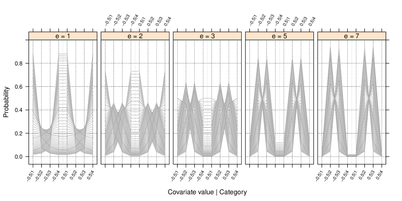
For evaluating the performance of the estimators, the probability of each of the tables has been calculated under model (14), for parameter values that are fixed according to the following scheme. The parameter $\beta$ takes values on some sufficiently fine equi-spaced grid in the interval $[-6,0]$. For $\beta$ in the interval $(0,6]$ the results can be predicted by the symmetry relations of Theorem 8.1. For each value of $\beta$, the nuisance parameters take values $(\alpha_{1},\alpha_{2},\alpha_{3})^{T}=e(-1,0,1)^{T}$ for $e\in\{1,2,3,5,7\}$. Figure 1 is a pictorial representation of the probability settings for the two multinomial vectors in the $2\times 4$ contingency table with fixed row totals, at each combination of values for $\beta$ and $(\alpha_{1},\alpha_{2},\alpha_{3})^{T}$. Under the above scheme for fixing parameter values, the probability of the end categories tends to zero as $e$ increases, and hence more extreme probability settings are being considered as $e$ grows.

The findings of the current complete enumeration exercise are outlined in the following Subsection. The same complete enumeration design has been applied to a number of settings, with $m_{1}\neq m_{2}$, with different link functions, with different numbers of categories, and/or for different non-symmetric specifications for the nuisance parameters (results not shown here) yielding qualitatively the same conclusions; the current setup merely allows a clear pictorial representation of the findings on the behaviour of the reduced-bias estimator. An R script that can produce the results of the current complete enumeration for any number of categories, any link function, any configuration of totals and any combination of parameter settings in $2\times k$ contingency tables is available in the supplementary material.

Figure 2: Probability of infinite estimates (top), conditional biases (middle) and conditional mean squared errors (bottom) of $\hat{\beta}$ and $\tilde{\beta}_{BC}$ for the parameter settings considered in the complete enumeration study.

8.3 Remarks on the results

Remark 1. On the estimates of $\alpha_{1}$, $\alpha_{2}$ and $\alpha_{3}$: According to Section 3, for data sets where a specific category $s\in\{1,2,3,4\}$ is observed for neither $x=-1/2$ nor $x=1/2$, the maximum likelihood estimate of $\alpha$ is on the boundary of the parameter space as follows:

$$\begin{array}[]{ll}s=1:&\hat{\alpha}_{1}=-\infty\\ s=2:&\hat{\alpha}_{2}=\hat{\alpha}_{1}\\ s=3:&\hat{\alpha}_{3}=\hat{\alpha}_{2}\\ s=4:&\hat{\alpha}_{3}=+\infty\\ \end{array}\,.$$

A least for log-concave $g(.)$, according to the results in Pratt (1981), the above equations extend directly to the case of any number of categories and number of covariate settings and can directly be used to check what happens when two or more categories are unobserved.

Nevertheless, the maximum likelihood estimator of $\beta$ is invariant to merging a non-observed category with either the previous or next category and can be finite even if some of the $\alpha$ parameters are on the boundary of the parameter space. Hence, maximum likelihood inferences on $\beta$ are possible even if a category is not observed. The same behaviour is observed for the reduced-bias estimators of $\alpha_{1},\alpha_{2},\alpha_{3}$ with the difference that if the non-observed category is $s=1$ and/or $s=4$, then $\tilde{\alpha}_{1,RB}$ and/or $\tilde{\alpha}_{3,RB}$ are finite. A special case of this observation has been encountered in Subsection 6.1 where reduction of the bias corresponds to adding $1/2$ to the end categories, guaranteeing the finiteness of the cumulative logits. Hence, there is no need for non-observed end-categories to be merged with the neighbouring ones when the reduced-bias estimator is used. If any of the other categories is empty, then the reduced-bias estimator of $\beta$ is invariant to merging those with any of the neighbouring ones.

It should be mentioned here that if both the second and the third category are empty then the reduced-bias estimate of $\beta$ and the generalized empirical logistic transform are identical. To see that, note that in the special case of logistic regression, the adjusted scores in Subsection 4.4 suggest adding half a leverage to each of $y_{r1}$ and $y_{r2}$ $(r=1,2)$ (this result for logistic regressions was obtained in Firth, 1993). Furthermore, the model with $q=1$ is saturated and hence both leverages are $1$. Hence the reduced-bias estimate of $\beta$ coincides with the generalized empirical logistic transform, which for $k=2$ is $\mathop{\rm log}\{(y_{11}+1/2)/(m_{1}-y_{11}+1/2)\}-\mathop{\rm log}\{(y_{21}+1/2)/(m_{2}-y_{21}+1/2)\}$.

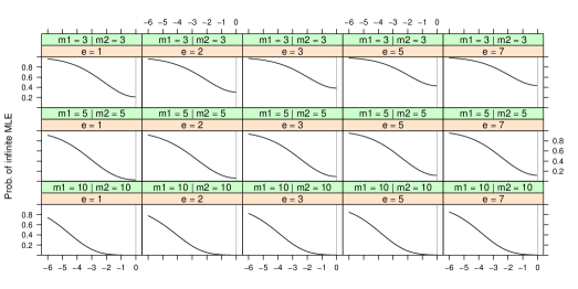
Remark 2. On $\hat{\beta}$ and $\tilde{\beta}_{BC}$: As is expected from the discussion in Section 3, the maximum likelihood estimator of $\beta$ is infinite for certain configurations of zeros on the table, and for such configurations the bias-corrected estimator is also undefined owing to its explicit dependence on the maximum likelihood estimator. Hence, for $\hat{\beta}$ and $\tilde{\beta}_{BC}$, the bias function is undefined and the mean squared error is infinite. A possible comparison of the performance of $\hat{\beta}$ and $\tilde{\beta}_{BC}$ is in terms of conditional bias and conditional mean squared error where the conditioning event is that $\hat{\beta}$ has a finite value.

For detecting parameters with infinite values the diagnostics in Lesaffre and Albert (1989, §4) for multinomial logistic regressions are adapted to the current setting. Data sets that result in infinite estimates for $\beta$ have been detected by observation of the size of the corresponding estimated standard error based on the inverse of the Fisher information, and by observation of the absolute value of the estimates when the convergence criteria were satisfied. If the standard error was greater than $200$ and the estimate was greater than $100$, then the estimate was labelled infinite. A second pass through the data sets has been performed making the convergence criterion for the Fisher scoring stricter than $|U_{t}({\boldsymbol{\delta}}^{c})|<10^{-10}$. The estimates that were labelled infinite using the aforementioned diagnostics, further diverged towards infinity while the rest of the estimates remained unchanged to high accuracy.

The probability of encountering an infinite $\hat{\beta}$ for the different possible parameter settings is shown at the top row of Figure 2. For $\beta\in(0,6)$ the probability of encountering an infinite value is simply a reflection of the probability in $(-6,0)$. As is apparent the probability of infinite estimates increases as $e$ increases and for each value of $e$ it increases as $|\beta|$ increases. As is natural as $m$ increases, the probability of encountering infinite estimates is reduced but is always positive.

Of course, the findings from the current comparison of $\hat{\beta}$ with $\tilde{\beta}_{BC}$ should be interpreted critically, bearing in mind the conditioning on the finiteness of $\hat{\beta}$; the comparison suffers from the fact that the first-order bias term that is required for the calculation of $\tilde{\beta}_{BC}$ is calculated unconditionally. The comparison is fairer when the probability of infinite estimates is small; this happens on a region around zero whose size also increases as $m$ increases.

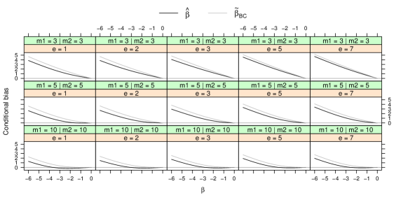
The conditional bias and conditional mean squared error of $\hat{\beta}$ and $\tilde{\beta}_{BC}$ are shown in the left and right of the second row of Figure 2. The identities in Theorem 8.1 apply also for the conditional and conditional mean squared error; to see this set $P$ to be the conditional probability of each table in the proof of Theorem 8.1. Hence, for $\beta\in(0,6)$, the conditional bias is simply a reflection of the conditional bias for $\beta\in(-6,0)$ across the $45^{o}$ line, and the conditional mean squared error is a reflection of the conditional mean squared error for $\beta\in(-6,0)$ across $\beta=0$.

Figure 3: Biases (top) and mean squared errors (bottom) of $\hat{\beta}_{EL}$ and $\tilde{\beta}_{RB}$ for the parameter settings considered in the complete enumeration study.

The behaviour of the estimators in terms of conditional bias is similar, with the maximum likelihood estimator performing slightly better than $\tilde{\beta}_{BC}$ for small $m$. As $m$ increases the bias corrected estimator starts performing better in terms of bias in a region around zero, where the probability of infinite estimates is smallest. The same is noted for the conditional mean squared error. The estimator $\tilde{\beta}_{BC}$ performs better than $\hat{\beta}$ in a region around zero, whose size increases as $m$ increases. The same behaviour as for $e=7$ persists for larger values of $e$ (figures not shown here).

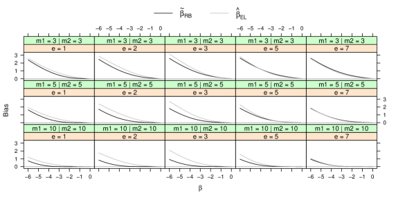
Remark 3. On $\hat{\beta}_{EL}$ and $\tilde{\beta}_{RB}$: The estimators $\hat{\beta}_{EL}$ and $\tilde{\beta}_{RB}$, always have finite value irrespective of the configuration of zeros on the table. Hence, in contrast to $\hat{\beta}$ and $\tilde{\beta}_{BC}$, a comparison in terms of their unconditional bias and unconditional mean squared error is possible. The left plot of Figure 3 shows the bias function of the estimator for the parameter settings considered in the complete enumeration study. For $\beta\in(0,6)$, the bias function is simply a reflection of the bias for $\beta\in(-6,0)$ across the $45^{o}$ line, and the mean squared error is a reflection of the mean squared error for $\beta\in(-6,0)$ across $\beta=0$.

The reduced-bias estimator performs better than $\hat{\beta}_{EL}$ in terms of bias for small values of $e$ and the differences in the bias functions diminish as $e$ increases. A similar limiting behaviour holds for their mean squared errors, though for small values of $e$, $\hat{\beta}_{EL}$ performs slightly better than $\tilde{\beta}_{BR}$ in terms of mean squared error in the range $(-4,4)$ and worse outside that range. The mean squared error of both estimators converges to zero as $m$ increases, which is what is expected from consistent estimators (see, Kosmidis, 2007a, §6.3 for a proof of the consistency of the reduced-bias estimator).

Figure 4: Coverage probabilities of nominally 95% asymptotic Wald-type confidence intervals for $\beta$, based on $\hat{\beta}$ and $\tilde{\beta}_{BC}$ (top) and $\hat{\beta}_{EL}$ and $\tilde{\beta}_{RB}$ (bottom) and the respective standard errors, for $\beta\in[-10,0)$ and $\alpha=e(-1,0,1)^{T}$ for $e\in\{1,2,3,5,7\}$.

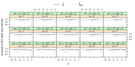
Remark 4. On the coverage of 95% Wald confidence intervals For a table $T$ and an estimator $\beta^{*}(T)$, consider the nominally $100(1-a)\%$ Wald-type confidence interval for $\beta$

$$\beta^{*}(T)\pm z_{1-a/2}S^{*}(T)\,,$$

where $z_{a}$ is the $100a$th quantile of a standard normal distribution and $S^{*}(T)$ is the estimator of the standard error of $\beta^{*}(T)$. For $\hat{\beta}$, $\tilde{\beta}_{BC}$ and $\tilde{\beta}_{RB}$, $S^{*}(T)$ is taken to be the square root of the diagonal element of the inverse of the Fisher information corresponding to $\beta$, evaluated at $\hat{\beta}(T)$, $\tilde{\beta}_{BC}(T)$ and $\tilde{\beta}_{RB}(T)$, respectively. For the estimation of the standard error for $\hat{\beta}_{EL}$, the variance formula given in McCullagh (1980, §2.3) is used. If the maximum likelihood estimate is infinite then we make the convention that the confidence intervals based on $\hat{\beta}$ and $\tilde{\beta}_{BC}$ are $(-\infty,\infty)$. Figure 4 shows the coverage probabilities of the four competing intervals for $\alpha=e(-1,0,1)^{T}$ with $e\in\{1,2,3,5,7\}$, and for $\beta\in[-10,0]$. The coverage probability for $\beta\in(0,10)$ is simply a reflection of the coverage probability for $\beta\in(-10,0)$ across $\beta=0$.

Wald-type confidence intervals based on the maximum likelihood estimator demonstrate a conservative behaviour in terms of coverage, and the coverage probability converges to $1$ as $|\beta|\to\infty$. Furthermore, the coverage probability seems to uniformly get closer to the nominal level as $m$ increases. The intervals based on the bias-corrected estimator also demonstrate a conservative behaviour in a neighbourhood around $\beta=0$, then tend to undercover for an interval of large $|\beta|$ values, and as for $\hat{\beta}$, when $|\beta|\to\infty$ the coverage probability tends to $1$.

A more dramatic undercoverage is present for confidence intervals based on $\hat{\beta}_{EL}$ when $|\beta|$ is large. Actually after some value of $|\beta|$ the confidence intervals based on $\hat{\beta}_{EL}$ completely lose coverage (the full range of the coverage probability is not shown here). On the other hand, those intervals behave satisfactorily around $\beta=0$. This behaviour relates to the fact that the variance estimator for $\hat{\beta}_{EL}$ is obtained under the assumption that $\beta=0$ and can seriously underestimate the variance of $\hat{\beta}_{EL}$ when $|\beta|$ is larger than about $1$ (the same observation is also made in McCullagh, 1980, §2.3). Furthermore, it is worth noting that the point where coverage is lost completely moves closer to zero as $m$ increases. Hence, use of Wald-type confidence intervals based on $\hat{\beta}_{EL}$ is not recommended in practical applications.

Apart from being conservative, confidence intervals based on $\tilde{\beta}_{RB}$ seem to behave better for a wider range of $\beta$ around zero, but also completely lose coverage after some value of $|\beta|$. The complete loss of coverage for large effects is due to an interplay of discreteness of the response and the fact that $\tilde{\beta}_{RB}$ and $\hat{\beta}_{EL}$ take always finite values. Specifically, for any finite $m$ there is only a finite number of possible Wald-type confidence intervals because the response is multinomially distributed, and any of those confidence intervals has finite endpoints. Therefore, there will always be a large enough value of $|\beta|$ which is not contained in any of the confidence intervals resulting to a complete loss of coverage. Nevertheless, in contrast to $\hat{\beta}_{EL}$, the coverage properties of the Wald-type confidence intervals based on $\hat{\beta}_{RB}$ improve quickly and the value where coverage is lost moves quickly away from zero as $m$ increases. This is because the cardinality of the set of the possible confidence intervals increases and the approximation of the necessarily discrete distribution of the reduced-bias estimator by a Normal distribution with variance the inverse of the Fisher information gets more accurate. This results in the increasing accuracy of the approximation of the distribution of the Wald-pivot by a Normal distribution.

As the current study demonstrates the Wald-type confidence intervals based on any of the estimators do not behave satisfactorily for the whole range of $\beta$ and for small sample sizes. For this reason current research focuses on alternative confidence intervals that can have one infinite endpoint (see Section 12). Until conclusive results are produced, Wald-type confidence intervals based on the reduced-bias estimator can still be used in practice as asymptotically correct, bearing in mind that, they will be generally slightly conservative for moderate effects (like the ones based on the maximum likelihood estimator) especially in small samples, and also that their coverage properties will deteriorate for extremely large effects.

9 Shrinkage towards a binomial model for the end-categories

Table 3 shows the maximum likelihood estimates, the reduced-bias estimates and the corresponding estimated standard errors from fitting a proportional odds model and a proportional hazards model of the form (14) to the artificial data considered in Example 6.1.

Table 3: Parameter estimates and corresponding estimated standard errors (in parenthesis) from fitting a proportional odds model and a proportional hazards model of the form (14) to the artificial data considered in Example 6.1, using maximum likelihood and bias reduction.

Model	Parameter	Maximum likelihood	Bias reduction
Proportional odds ($G(\eta)=\exp(\eta)/\{1+\exp(\eta)\}$)	$\beta$	-1.944 (0.895)	-1.761 (0.850)
	$\alpha_{1}$	1.187 (0.449)	1.084 (0.428)
	$\alpha_{2}$	3.096 (0.787)	2.781 (0.701)
	$\alpha_{3}$	$\infty$ ($\infty$)	4.457 (1.440)
Proportional hazards ($G(\eta)=1-\exp\{-\exp(\eta)\}$)	$\beta$	-0.689 (0.401)	-0.635 (0.389)
	$\alpha_{1}$	0.313 (0.220)	0.297 (0.219)
	$\alpha_{2}$	1.097 (0.260)	1.013 (0.246)
	$\alpha_{3}$	$\infty$ ($\infty$)	1.518 (0.357)

There is apparent shrinkage of the reduced-bias estimates towards zero, which implies a shrinkage of the cumulative probabilities towards $G(0)$. This implies a shrinkage of the probabilities for the first and the last category of the ordinal scale towards $G(0)$ and $1-G(0)$ respectively, and a corresponding shrinkage of the probabilities of the intermediate categories towards zero.

To investigate further the apparent shrinkage effect, the maximum likelihood and reduced-bias estimates of proportional odds and proportional hazards models of the form (14) are obtained for every possible $2\times 6$ table with row totals $m_{1}=m_{2}=3$. This setting is chosen because it is one that results in sparse tables, allowing the construction of plots of fitted probabilities that are not massively overcrowded (under this setting there are $3136$ tables to be estimated).

For each category of the ordinal response, Figure 5 shows the fitted probabilities based on the reduced-bias estimator against the fitted probabilities based on the maximum likelihood estimator. The grey areas are where the points would all be expected to lie if the shrinkage relationships were strictly satisfied for each pair of fitted probabilities. Clearly this is not the case.

The points on the plots for the first category roughly lie slightly above the $45^{o}$ line for fitted values less than $G(0)$, and slightly below it for fitted values greater than $G(0)$. The points for the last category exhibit similar behaviour but with $G(0)$ replaced by $1-G(0)$. The shrinkage effect appears to be stronger the further the probability is from the shrinkage points $G(0)$ and $1-G(0)$.

The points on the plots for the intermediate categories lie mostly under the $45^{o}$ line, except in cases where the maximum likelihood fitted probability is very close to zero. Hence, the fitted probabilities for the intermediate categories based on the reduced-bias estimator tend to shrink towards zero. The plots also suggest that the further the probability is from zero the stronger is the shrinkage effect.

Figure 5: The fitted probabilities based on the reduced-bias estimator ($\tilde{\pi}_{s}$) against the fitted probabilities based on the maximum likelihood estimator ($\hat{\pi}_{s}$), for each category of the response. The top row corresponds to the proportional odds model and the bottom to a proportional hazards model. The grey areas are where the points would be expected to lie if shrinkage was strict.

The shrinkage properties observed here are a direct generalization of the shrinkage that is implied by improving bias in the estimation of binomial logistic regression models (Copas, 1988; Cordeiro and McCullagh, 1991; Firth, 1992) to links other than the logistic and to models with ordinal responses.

Corresponding empirical investigations of shrinkage based on both complete enumerations and simulations under models fitted to real data have also been performed but are not shown here. The results are qualitatively the same: reduction of bias in cumulative link models shrinks the multinomial model towards a binomial model that has probability $G(0)$ for the first category and probability $1-G(0)$ for the last category.

10 A simulation study

In order to further illustrate the properties of the reduced-bias estimator in more complex scenarios than the one in the complete enumeration study of Section 8, a simulation study is set-up based on part of the data that has been analyzed in Jackman (2004). The data is publicly available through the R package pscl (Jackman, 2012) and seems to agree with the data available for rater F1 in the analysis in Jackman (2004). The data contains the score of rater F1 for 106 applications to the Political Science PhD Program at Stanford University along with corresponding applicant-specific observations. The rater’s score is on a five-point integer-valued ordinal scale from $1$ to $5$, with $1$ indicating the lowest rating and $5$ indicating the highest rating. Consider that the cumulative log-odds for rating $s$ for the $r$th candidate is modelled as

$$\mathop{\rm log}\frac{\gamma_{rs}}{1-\gamma_{rs}}=\alpha_{s}-\beta_{1}x_{r1}-\beta_{2}x_{r2}-\beta_{3}z_{r1}-\beta_{4}z_{r2}-\beta_{5}g_{r}\quad(r=1,\ldots,106;s=1,\ldots,4)\,,$$ (16)

where $x_{r1}$ and $x_{r2}$ are the $r$th applicant’s scores on the quantitative and verbal section of the GRE, respectively (after subtracting the respective mean and dividing by the respective standard deviation), $z_{r1}$ and $z_{r2}$ are dummy variables indicating whether the $r$th applicant has an interest in American politics and Political Theory, respectively (with $1$ representing a positive reply and $0$ a negative one), and $g_{r}$ is the gender of the $r$th applicant $(r=1,\ldots,106)$. The parameter $\alpha_{1},\ldots,\alpha_{5}$ are the cutpoints and $\beta_{1},\ldots,\beta_{5}$ describe the effect of the corresponding applicant-specific covariates on the cumulative log-odds.

Table 4: Estimated biases, mean-squared errors (MSE) and coverage probabilities of $95\%$ Wald-type confidence intervals from a simulation of size $10^{5}$ under the maximum likelihood fit of model (16). The last column shows the estimated relative increase of the mean squared error from its absolute minimum (the variance) due to bias. The relative increase of the mean squared error is the square of the bias divided by the variance. The estimated simulation error is less than 0.004 for the bias and the MSE estimates and less than 0.001 for the coverage estimates.

Method	Parameter	Bias	MSE	Coverage	Bias2/Variance (in %)
Maximum likelihood	$\beta_{1}$	0.132	0.142	0.943	13.928
	$\beta_{2}$	0.055	0.062	0.943	5.203
	$\beta_{3}$	0.208	0.722	0.947	6.347
	$\beta_{4}$	0.004	0.630	0.944	0.003
	$\beta_{5}$	0.077	0.238	0.944	2.569
Bias correction	$\beta_{1}$	-0.001	0.106	0.948	0.002
	$\beta_{2}$	0.001	0.051	0.953	0.001
	$\beta_{3}$	-0.004	0.577	0.954	0.002
	$\beta_{4}$	0.003	0.551	0.956	0.001
	$\beta_{5}$	0.001	0.205	0.954	0.000
Bias reduction	$\beta_{1}$	0.002	0.107	0.949	0.002
	$\beta_{2}$	0.002	0.051	0.953	0.007
	$\beta_{3}$	0.002	0.579	0.954	0.001
	$\beta_{4}$	0.004	0.553	0.956	0.003
	$\beta_{5}$	0.003	0.205	0.954	0.003

Model (16) is fitted using maximum likelihood and the maximum likelihood estimates of $\beta_{1},\ldots,\beta_{5}$ are $1.993$, $0.892$, $2.816$, $0.009$, $1.215$ respectively indicating that an increase in the value of any of the covariates is associated with higher probability for high ratings holding all else in the model fixed. Then an extensive simulation under the maximum likelihood fit is performed for estimating the biases, mean squared errors and coverage probabilities of Wald-type $95\%$ confidence intervals for $\beta_{1},\ldots,\beta_{5}$ when maximum likelihood, bias correction and bias reduction is used. There have been instances of simulated data sets where one or more rating categories were empty. In those cases, empty categories were merged with neighbouring ones according to the discussion in Remark 1 of Section 8. The results are shown on Table 4. There was only one data set for which the maximum likelihood estimate of $\beta_{3}$ was $+\infty$. This data set was excluded when estimating the bias, mean squared error and coverage probability for the maximum likelihood and the bias-corrected estimator and hence the corresponding figures in the table estimate the conditional respective quantities (that is given that the maximum likelihood estimator has finite value). On the other hand, the reduced-bias estimates were finite for all datasets and hence the corresponding figures are estimates of the targeted unconditional quantities. In this particular setting, the probability of the conditioning event is rather small and a direct comparison of the estimated conditional and unconditional quantities can be informative.

Temporarily ignoring the fact that the maximum likelihood estimator can be infinite, both the bias corrected and reduced bias estimators perform equally well in the current study. Furthermore, the figures in Table 4 demonstrate a significant reduction both in terms of bias and mean squared error when either bias correction or bias reduction is used. In the current study the effect of estimation bias is quite significant; the mean squared errors of the components of the maximum likelihood estimator are inflated by as much as $13.9\%$ due to bias from their minimum values (the variances). The corresponding inflation factors for the bias corrected and reduced-bias estimators are quite close to zero, which when combined with the observed reduction in mean squared error illustrates the benefits that the reduction of bias can have in the estimation of such models. Lastly, a slight improvement in the coverage properties of Wald-type confidence intervals is observed when the bias is corrected.

Overall and taking into account that the reduced-bias estimator is always finite the current study illustrates its superior frequentist properties from the alternatives.

11 Wine tasting data

Table 5: The reduced-bias estimates for the parameters of model (1), the corresponding estimated standard errors (in parenthesis) and the values of the $Z$ statistic for the hypothesis that the corresponding parameter is zero.

Parameter	RB estimates		$Z$ statistic
$\alpha_{1}$	-1.19	(0.50)	-2.40
$\alpha_{2}$	1.06	(0.44)	2.42
$\alpha_{3}$	3.50	(0.74)	4.73
$\alpha_{4}$	5.20	(1.47)	3.52
$\beta_{1}$	2.62	(1.52)	1.72
$\beta_{2}$	2.05	(0.58)	3.54
$\beta_{3}$	2.65	(0.75)	3.51
$\beta_{4}$	2.96	(1.50)	1.98
$\theta$	1.40	(0.46)	3.02

The partial proportional odds model of Example 1.1 is here refitted using the reduced-bias estimator. The result is shown in Table 5. All estimates and estimated standard errors are finite. A Wald statistic for testing departures from the assumption of proportional odds via departures from the hypothesis $\beta_{1}=\beta_{2}=\beta_{3}=\beta_{4}$ is

$$W=(L\tilde{\boldsymbol{\beta}}_{RB})^{T}I(\tilde{\boldsymbol{\delta}}_{RB})L\tilde{\boldsymbol{\beta}}_{RB}\,,$$

where

$$L=\left[\begin{array}[]{cccc}1&0&0&-1\\ 0&1&0&-1\\ 0&0&1&-1\end{array}\right]$$

is a matrix of contrasts of $\beta$. The matrix

$$I({\boldsymbol{\delta}})=\left\{LF^{{\boldsymbol{\beta}}{\boldsymbol{\beta}}}({\boldsymbol{\delta}})L^{T}\right\}^{-1}\,,$$

is the inverse of the variance-covariance matrix of the asymptotic distribution of $L\tilde{\boldsymbol{\beta}}_{RB}$, where $F^{{\boldsymbol{\beta}}{\boldsymbol{\beta}}}({\boldsymbol{\delta}})$ is the ${\boldsymbol{\beta}}$-block of the inverse of the Fisher information. By the asymptotic normality of $\tilde{\boldsymbol{\beta}}_{RB}$, $W$ has an asymptotic $\chi^{2}$ distribution with $3$ degrees of freedom. The value of $W$ for the data in Table 1 is $0.7502$ leading to a $p$-value of $0.861$, which provides no evidence against the proportional odds assumption. This is also apparent from Table 5 where the reduced-bias estimates of $\beta_{1},\beta_{2},\beta_{3},\beta_{4}$ are comparable in value.

It is worth noting that, in contrast to the output reported in Example 1.1, the values of the $Z$ statistics for $\alpha_{4}$, $\beta_{1}$ and $\beta_{4}$ are far from being exactly zero.

12 Concluding remarks and further work

Based on the results of the complete enumeration study, $\tilde{\beta}_{RB}$ appears to be always finite in contrast to $\hat{\beta}_{ML}$ and $\tilde{\beta}_{BC}$, and also to have comparable behaviour to $\hat{\beta}_{EL}$ in terms of bias and mean squared error. Furthermore, Wald-type asymptotic confidence intervals based on $\tilde{\beta}_{RB}$ behave satisfactorily, maintaining good coverage properties for a wide range of $\beta$ values. A complete loss of coverage is still present but the point where this happens is far away from zero and diverges as the number of observations increases. The application of the current complete enumeration setup for complementary log-log and probit link functions, for varying values of the row totals, and for different numbers of categories, resulted in qualitatively the same conclusions.

In Remark 1 of the complete enumeration study, the finiteness of the reduced-bias estimates for $\alpha_{1}$ and/or $\alpha_{q}$ was noted even in cases where the first and/or last category of the ordinal variable is not observed. This behaviour has been also encountered in the simulation study of Section 10 and in all of the many settings where the reduced-bias estimator has been applied, and is defensible from an experimental point of view. When the experimenter sets an ordinal scale, the end-categories of that scale largely determine the possible responses. Hence, one might argue that the end categories should play a bigger role than the intermediate categories in the analysis, and a good estimation method should not be as democratic as maximum likelihood is in this respect; accepting that the ordinal scale is well-defined, if an end category is not observed then it seems more appropriate to slightly inflate its probability of occurrence, instead of setting it to zero as the maximum likelihood estimator would do.

The latter point of view does not only apply for non-observed end-categories. It applies to all analyses of ordinal data through cumulative link models and is reinforced by the fact that an improvement in the frequentist properties of the maximum likelihood estimator resulted in the shrinkage of the cumulative link model towards a binomial model for the end-categories.

The above observations, along with the fact that $\tilde{\boldsymbol{\delta}}_{RB}$ respects the invariance properties of the cumulative link model and can be easily obtained using the procedures in Section 5, provide a strong case for its routine use in the estimation of cumulative link models.

Laara and Matthews (1985) demonstrate the equivalence of continuation ratio models with complementary log-log link and proportional hazards models in discrete time. Hence, the reduced-bias estimates for the regression parameters of the former can be obtained by using the results in the current paper for the latter.

The investigation of confidence intervals that maintain good properties without suffering from a complete loss of coverage for extreme effects is the subject of future work. Current research focuses on the use of profiles of the asymptotic pivot $\{U^{*}({\boldsymbol{\delta}})\}^{T}F^{-1}({\boldsymbol{\delta}})U^{*}({\boldsymbol{\delta}})$ which can be shown to have an asymptotic $\chi^{2}$ distribution, and the combination of the resultant intervals with the profile likelihood intervals. In this way confidence intervals with one infinite endpoint are possible and are suggested to accompany the reduced-bias estimator which appears always to take finite value. Such intervals seem to better reflect uncertainty when extreme settings are considered, and lead to improved coverage properties without loss of coverage.

As is done in Subsection 11, comparison of nested models can be performed using asymptotic Wald-type test based on the reduced-bias estimator. Another option is the use of the adjusted score statistic

$$\{U^{*}(\tilde{\boldsymbol{\delta}}_{-})\}^{T}F^{-1}(\tilde{\boldsymbol{\delta}}_{-})U^{*}(\tilde{\boldsymbol{\delta}}_{-})\,,$$

where $\tilde{\boldsymbol{\delta}}_{-}$ are the estimates under the hypothesis that results in the smaller model, and $U^{*}({\boldsymbol{\delta}})$ and $F({\boldsymbol{\delta}})$ are the vector of adjusted score functions and the Fisher information of the larger model, respectively. The fact that $U^{*}({\boldsymbol{\delta}})=U({\boldsymbol{\delta}})+A({\boldsymbol{\delta}})$ where $A({\boldsymbol{\delta}})=O(1)$ guarantees an asymptotic $\chi^{2}$ distribution for that statistic. For the example in Subsection 11 the value of the adjusted score statistic is $0.9357$ on $3$ degrees of freedom giving a $p$-value of 0.8168 which leads to qualitatively the same conclusion as that of the Wald test. When testing departures from the proportional odds assumption in general, the adjusted score statistic has the same disadvantage as the ordinary score statistic; the Fisher information matrix for the partial proportional odds model can be non-invertible when evaluated at the estimates of the corresponding proportional odds model.

Supplementary material

The accompanying supplementary material includes an R script (R Development Core Team, 2012) that can be used to produce the results of the complete enumeration study for any number of categories, any link function and any configuration of row totals in contingency tables. The current version of the R function bpolr is also included. The bpolr function fits cumulative link models and their extensions with dispersion effects either by maximum likelihood, or bias reduction or bias correction. An updated version of the function will be part of the next major release of the R package brglm (Kosmidis, 2007b). Scripts that reproduce the data analyses undertaken in the paper are also available in the supplementary material.

References

- Agresti (2010) Agresti (2010). Analysis of Ordinal Categorical Data (2nd Edition). John Wiley & Sons.
- Albert and Anderson (1984) Albert, A. and J. Anderson (1984). On the existence of maximum likelihood estimates in logistic regression models. Biometrika 71(1), 1–10.
- Anscombe (1956) Anscombe (1956). On estimating binomial response relations. Biometrika 43(3), 461–464.
- Bull et al. (2002) Bull, S. B., C. Mak, and C. Greenwood (2002). A modified score function estimator for multinomial logistic regression in small samples. Computational Statistics and Data Analysis 39, 57–74.
- Christensen (2012a) Christensen, R. H. B. (2012a). ordinal — A tutorial on fitting cumulative link models with the ordinal package. R package version 2012.01-19 http://www.cran.r-project.org/package=ordinal/.
- Christensen (2012b) Christensen, R. H. B. (2012b). ordinal—regression models for ordinal data. R package version 2012.01-19 http://www.cran.r-project.org/package=ordinal/.
- Clogg et al. (1991) Clogg, C. C., D. B. Rubin, N. Schenker, B. Schultz, and L. Weidman (1991). Multiple imputation of industry and occupation codes in census public-use samples using Bayesian logistic regression. Journal of the American Statistical Association 86, 68–78.
- Copas (1988) Copas, J. B. (1988). Binary regression models for contaminated data (with discussion). Journal of the Royal Statistical Society, Series B: Methodological 50(2), 225–265.
- Cordeiro and McCullagh (1991) Cordeiro, G. M. and P. McCullagh (1991). Bias correction in generalized linear models. Journal of the Royal Statistical Society, Series B: Methodological 53(3), 629–643.
- Cox and Reid (1987) Cox, D. R. and N. Reid (1987). Parameter orthogonality and approximate conditional inference. Journal of the Royal Statistical Society, Series B: Methodological 49, 1–18.
- Cox and Snell (1989) Cox, D. R. and E. J. Snell (1989). Analysis of Binary Data (2nd ed.). London: Chapman and Hall.
- Efron (1975) Efron, B. (1975). Defining the curvature of a statistical problem (with applications to second order efficiency) (with discussion). The Annals of Statistics 3, 1189–1217.
- Firth (1992) Firth, D. (1992). Generalized linear models and Jeffreys priors: An iterative generalized least-squares approach. In Y. Dodge and J. Whittaker (Eds.), Computational Statistics I, Heidelberg. Physica-Verlag.
- Firth (1993) Firth, D. (1993). Bias reduction of maximum likelihood estimates. Biometrika 80(1), 27–38.
- Gart et al. (1985) Gart, J. J., H. M. Pettigrew, and D. G. Thomas (1985). The effect of bias, variance estimation, skewness and kurtosis of the empirical logit on weighted least squares analyses. Biometrika 72, 179–190.
- Gart and Zweifel (1967) Gart, J. J. and J. R. Zweifel (1967). On the bias of various estimators of the logit and its variance with application to quantal bioassay. Biometrika 54(1), 181–187.
- Haberman (1980) Haberman, S. J. (1980). Discussion of McCullagh (1980). Journal of the Royal Statistical Society, Series B: Methodological 42, 136–137.
- Haldane (1955) Haldane, J. (1955). The estimation of the logarithm of a ratio of frequencies. Annals of Human Genetics 20, 309–311.
- Heinze and Schemper (2002) Heinze, G. and M. Schemper (2002). A solution to the problem of separation in logistic regression. Statistics in Medicine 21, 2409–2419.
- Hitchcock (1962) Hitchcock, S. E. (1962). A note on the estimation of parameters of the logistic function using the minimum logit method. Biometrika 49(1), 250–252.
- Jackman (2004) Jackman, S. (2004). What do we learn from graduate admissions committees? a multiple rater, latent variable model, with incomplete discrete and continuous indicators. Political Analysis 12(4), 400–424.
- Jackman (2012) Jackman, S. (2012). pscl: Classes and methods for R developed in the Political Science Computational Laboratory, Stanford University. R package version 1.04.4 URL http://pscl.stanford.edu/.
- Kosmidis (2007a) Kosmidis, I. (2007a). Bias reduction in exponential family nonlinear models. Ph. D. thesis, Department of Statistics, University of Warwick. Available at http://www.ucl.ac.uk/~ucakiko.
- Kosmidis (2007b) Kosmidis, I. (2007b). brglm: Bias reduction in binomial-response glms. R package version 0.5-6 (2011-08-17), http://www.ucl.ac.uk/~ucakiko/software.html.
- Kosmidis (2009) Kosmidis, I. (2009). On iterative adjustment of responses for the reduction of bias in binary regression models. Technical Report 09-36, CRiSM working paper series.
- Kosmidis and Firth (2009) Kosmidis, I. and D. Firth (2009). Bias reduction in exponential family nonlinear models. Biometrika 96(4), 793–804.
- Kosmidis and Firth (2010) Kosmidis, I. and D. Firth (2010). A generic algorithm for reducing bias in parametric estimation. Electronic Journal of Statistics 4, 1097–1112.
- Kosmidis and Firth (2011) Kosmidis, I. and D. Firth (2011). Multinomial logit bias reduction via the poisson log-linear model. Biometrika 98(3), 755–759.
- Laara and Matthews (1985) Laara, E. and J. N. S. Matthews (1985). The equivalence of two models for ordinal data. Biometrika 72(1), 206–207.
- le Cessie and van Houwelingen (1992) le Cessie, S. and J. C. van Houwelingen (1992). Ridge estimators in logistic regression. Applied Statistics 41, 191–201.
- Lesaffre and Albert (1989) Lesaffre, E. and A. Albert (1989). Partial separation in logistic discrimination. Journal of the Royal Statistical Society, Series B: Methodological 51(1), 109–116.
- McCullagh (1980) McCullagh, P. (1980). Regression models for ordinal data. Journal of the Royal Statistical Society, Series B: Methodological 42, 109–142.
- Mehrabi and Matthews (1995) Mehrabi, Y. and J. N. S. Matthews (1995). Likelihood-based methods for bias reduction in limiting dilution assays. Biometrics 51, 1543–1549.
- Peterson and Harrell (1990) Peterson, B. and J. Harrell, Frank E. (1990). Partial proportional odds models for ordinal response variables. Applied Statistics 39, 205–217.
- Pratt (1981) Pratt, J. W. (1981). Concavity of the log likelihood (Corr: V77 p954). Journal of the American Statistical Association 76, 103–106.
- R Development Core Team (2012) R Development Core Team (2012). R: A Language and Environment for Statistical Computing. Vienna, Austria: R Foundation for Statistical Computing. ISBN 3-900051-07-0.
- Randall (1989) Randall, J. H. (1989). The analysis of sensory data by generalised linear model. Biometrical Journal 7, 781–793.
- Usmani (1994) Usmani, R. A. (1994). Inversion of Jacobi’s tridiagonal matrix. Computers & Mathematics with Applications 27(8), 59—66.