Estimating Rigid Transformation Between Two Range Maps Using Expectation Maximization Algorithm

Abstract

We address the problem of estimating a rigid transformation between two point sets, which is a key module for target tracking system using Light Detection And Ranging (LiDAR). A fast implementation of Expectation-maximization (EM) algorithm is presented whose complexity is $O(N)$ with $N$ the number of scan points.

I INTRODUCTION

Rigid registration of two sets of points sampled from a surface has been widely investigated (e.g., [1, 4, 9, 5, 6]) in computer vision literature. Generally, these methods are designed to tackle range maps with dense points for non-realtime applications.

In [2, 8] scans are matched using iterative closest line (ICL), a variant of “normal-distance” form of ICP algorithm [1] originally proposed in computer vision community by [3]. However, the convergence of this approach is sensitive to errors in normal direction estimations [10].

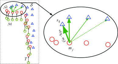
Figure 1: Illustration of the proposed algorithm.

Fig. 1 illustrates the concept. The light green circles denote the contour of a target $\mathcal{M}$. The red circles are the projection of $\mathcal{M}$ under a rigid transformation $T$, denoted as $\tilde{\mathcal{M}}$. Let $\mathcal{S}$ be the current range image shown as upper triangles. We propose an Expectation-maximization (EM) algorithm [7, 4] to find the rigid transformation such that the projected range image best matches the current image. Each point $m_{j}$ in $\tilde{\mathcal{M}}$ is treated as the center of a Parzen window. There is an edge between $s_{k}\in\mathcal{S}$ and $m_{j}$ if $s_{k}$ lies in the window. The weight of the edge $(s_{k},m_{j})$ is based on the proximity between the two vertices. The larger weight of the edge, the thicker the line is shown, and the more force that pulls the corresponding the point $m_{j}$ to $s_{k}$ through $T$.

This document describes a fast implementation of expectation maximization (EM) algorithm [7] to locally match between $\mathcal{M}$ and $\mathcal{S}$. By exploiting the sparsity of the locally matching matrix, this implementation scales linearly with the number of points.

II ALGORITHM DERIVATION

This section is devoted to the problem of how to estimate the rigid transformation $T$ using (EM) algorithm, giving scan map $\mathcal{S}$ and a contour model $\mathcal{M}$.

We constructed a bipartite graph $B=(\mathcal{M},\mathcal{S},E_{B})$ between the vertex set $\mathcal{M}$ to $\mathcal{S}$ with $E_{B}$ the set of edges. Let $m\in\mathcal{M}$ and $s\in\mathcal{S}$. An edge exists between the points $s$ and $m$ if and only if $\|s-m\|<W$ with $W$ a distance threshold. By $\mathcal{N}(s)\equiv\{m\mid(s,m)\in E_{B}\}$ we denote the neighborhood of $s$.

Scan points are indexed using a lookup hash-table with $W/2$ resolution. Find the points $m$ near a point $s$ within the radius $W$ involving searching through all the three-by-three neighbor grid of the cell containing $s$. Since hash table is used, and $|\mathcal{N}(s)|$ is bounded, construction graph $B$ is an $O(N)$ operation with $N$ the number of points in a scan.

Let $s_{j}\in\mathcal{S}$ be one of the $n_{\mathcal{S}}$ scan points, and $m_{k}\in\mathcal{M}$ be one of the $n_{\mathcal{M}}$ points from the model. We denote $T$ a rigid transformation from the model to the new scan frame, with the parameter vector $\mathbf{y}$. If $s_{j}$ is the measure of $m_{k}$ (i.e., $(s_{j},m_{k})\in\mathcal{B}$) with a known noise model, we write the density function as $p(s_{j}\mid m_{k},\mathbf{y})=p(s_{j}\mid T(m_{k},\mathbf{y}))$. In case of an additive and centered Gaussian noise of precision matrix $\Gamma$, $p(s_{j}\mid m_{k},T)=c\exp(-\frac{\|s_{j}-T(m_{k},\mathbf{y})\|_{\Gamma}^{2}}{2})$ where the Mahalanobis norm is defined as $\|x\|_{\Gamma}^{2}\equiv x^{T}\Gamma x$.

We use the binary matrix $A$ to represent the correspondence between $s_{j}$ and $m_{k}$. The entry $A_{jk}=1$ if $s_{j}$ matches $m_{k}$ and 0 otherwise. Assume each scan point $s_{j}$ corresponds to at most one model point. We have

$$\Sigma_{k}A_{jk}=\left\{\begin{array}[]{l}1~{}~{}\mbox{If }\mathcal{N}(s_{j})\neq\emptyset\\ 0~{}~{}\mbox{Otherwise.}\end{array}\right.$$

for all scan point index $j$.

For the above equation, we note that for the case $\mathcal{N}(s_{j})=\emptyset$, $s_{j}$ is an outlier, and the correspondence $s_{j}$ to $m_{k}$ can be treated as a categorical distribution. In order to apply EM procedure we use a random matching matrix $\mathcal{A}$ with each element a binary random variable. Each eligible matching matrix $A$ has a probability $p(A)\equiv p(\mathcal{A}=A)$. One can verify that $\bar{A}_{jk}=\mbox{E}\{\mathcal{A}_{jk}\}=P(\mathcal{A}_{jk}=1)$, and the following constraint holds

$$\Sigma_{k}\bar{A}_{jk}=\left\{\begin{array}[]{l}1~{}~{}\mbox{If }\mathcal{N}(s_{j})\neq\emptyset\\ 0~{}~{}\mbox{Otherwise.}\end{array}\right.$$

Considering the distribution of $\mathcal{A}_{j}$, the $j$-th row of the $\mathcal{A}$, which is the distribution of assigning the scan point $s_{j}$ to the model point $m_{k}$, i.e.,

$$p(\mathcal{A}_{j})=\prod_{m_{k}\in\mathcal{N}(s_{j})}(\bar{A}_{jk})^{\mathcal{A}_{jk}}$$

Assuming the scan points are independent, we can write

$$p(\mathcal{A})=\prod_{s_{j}\in\mathcal{S}}\prod_{m_{k}\in\mathcal{N}(s_{j})}(\bar{A}_{jk})^{\mathcal{A}_{jk}}=\prod_{(s_{j},m_{k})\in E_{\mathcal{B}}}(\bar{A}_{jk})^{\mathcal{A}_{jk}}$$ (1)

An example of $p(\mathcal{A})$ is the noninformative prior probability of the matches: a probability distribution that a given scan point is a measure of a given model point without knowing measurement information:

$$\bar{A}_{jk}=\pi_{jk}=\left\{\begin{array}[]{l}\frac{1}{|\mathcal{N}(s_{j})|}~{}~{}\mbox{If }\mathcal{N}(s_{j})\neq\emptyset\\ 0~{}~{}\mbox{Otherwise.}\end{array}\right.$$

The joint probability of the scan point $s_{j}$ and the corresponding assignment $\mathcal{A}_{j}$ can be expressed as

$$p(s_{j},\mathcal{A}_{j}\mid\mathcal{M},\mathbf{y})=\prod_{m_{k}\in\mathcal{N}(s_{j})}(\pi_{jk}p(s_{j}\mid m_{k},\mathbf{y}))^{\mathcal{A}_{jk}}$$

Providing that the scan points are conditionally independent, the overall joint probability is the product of the each row of $A$:

$$p(\mathcal{S},\mathcal{A}\mid\mathcal{M},\mathbf{y})=\prod_{(s_{j},m_{k})\in E_{\mathcal{B}}}(\pi_{jk}p(s_{j}\mid m_{k},\mathbf{y}))^{\mathcal{A}_{jk}}$$ (2)

and the logarithm of marginal distribution can be written as

$$\mbox{ML}(T)=\log p(\mathcal{S}\mid\mathcal{M},\mathbf{y})=\log\left(\sum_{\mathcal{A}}p(\mathcal{S},\mathcal{A}\mid\mathcal{M},\mathbf{y})\right)$$ (3)

Unfortunately, Eq. (3) has no closed-form solution and no robust and efficient algorithm to directly minimize it with respect to the parameter $\mathbf{y}$. Noticing that Eq. (3) only involves the logarithm of a sum, we can treat the matching matrix $\mathcal{A}$ as latent variables and apply the EM algorithm to iteratively estimate $\mathbf{y}$. Assuming after $n$-th iteration, the current estimate for $\mathbf{y}$ is given by $\mathbf{y}_{n}$, we can compute an updated estimate $T$ such that $\mbox{ML}(T)$ is monotonically increasing, i.e.,

$$\Delta(\mathbf{y}\mid\mathbf{y}_{n})=\mbox{ML}(\mathbf{y})-\mbox{ML}(\mathbf{y}_{n})>0$$

Namely, we want to maximize the difference $\Delta(\mathbf{y}\mid\mathbf{y}_{n})$.

Now we are ready to state two propositions whose proofs are relegated to Appendix.

Proposition II.1

$$\Delta(\mathbf{y}\mid\mathbf{y}_{n})=\mbox{E}_{\mathcal{A}\mid\mathcal{S},\mathcal{M},\mathbf{y}_{n}}\{\log\left({p(\mathcal{S},\mathcal{A}\mid\mathcal{M},\mathbf{y})}\right)\}$$

Proposition II.2

Given the transformation estimate $\mathbf{y}_{n}$, scan points $\mathcal{S}$ and model points $\mathcal{M}$, the posterior of the matching matrix $A$ can be written as

$$p(\mathcal{A}\mid\mathcal{S},\mathcal{M},\mathbf{y}_{n})=\prod_{j,k:(s_{j},m_{k})\in E_{\mathcal{B}}}(\hat{A}_{jk})^{\mathcal{A}_{jk}}$$ (4)

where

$$\mbox{E}{\{\mathcal{A}\}_{jk}}=\hat{A}_{jk}=\left\{\begin{array}[]{l}\frac{\pi_{jk}p(s_{j}\mid m_{k},\mathbf{y}_{n})}{\sum_{k}\pi_{jk}p(s_{j}\mid m_{k},\mathbf{y}_{n})}~{}~{}\text{If }\mathcal{N}(s_{j})\neq\emptyset\\ 0~{}~{}\text{Otherwise.}\end{array}\right.$$ (5)

Therefore, we have the following EM algorithm to compute $\mathbf{y}$ that maximizes the likelihood defined in Eq. (3). We assume there exists an edge in the graph $\mathcal{B}$ between $s_{j}$ and $m_{k}$ in the following derivation.

• E-step: Given the previous estimate $T_{n}$, we update $\hat{A}_{jk}$ using Eq. (5). The conditional expectation is computed as

  $$\Delta(\mathbf{y}\mid\mathbf{y}_{n}) =\mbox{E}_{\mathcal{A}\mid\mathcal{S},\mathcal{M},\mathbf{y}_{n}}\left\{\log p(\mathcal{S},\mathcal{A}\mid\mathcal{M},\mathbf{y})\right\}$$

  $$=\mbox{E}\left\{\log\left(\prod_{j,k}\pi_{jk}p(s_{j}\mid m_{k},\mathbf{y})^{\mathcal{A}_{jk}}\right)\right\}$$

  $$=\sum_{j,k}\mbox{E}\{\mathcal{A}_{jk}\}(\log p(s_{j}\mid m_{k},\mathbf{y})+\log\pi_{jk})$$

  $$=\sum_{j,k}\hat{A}_{jk}\|s_{j}-T(m_{k},\mathbf{y})\|_{\Gamma}^{2}+\mbox{const.}$$ (6)

  where E is $\mbox{E}_{\mathcal{A}\mid\mathcal{S},\mathcal{M},\mathbf{y}_{n}}$ in short, and const. is the terms irrelevant to $\mathbf{y}$.

• M-step: Compute $\mathbf{y}$ to maximize the least-squares expression in Eq. (6).

The above EM procedure is repeated until the model is converged, i.e., the difference of log-likelihood between two iterations $\Delta(\mathbf{y}\mid\mathbf{y}_{n})$ is less than a small number. The complexity of the above computation for a target in each iteration is $O(|E_{\mathcal{B}}|)$. Since the number of neighbors for $s_{j}$ is bounded, the complexity is reduced to $O(|\mathcal{S}|)$. Since experimental result shows that only 4-5 epochs are needed for EM iteration to converge. Consequently, the overall complexity for all of the tracked objects is $O(N)$ with $N$ the number of scan points.

The following proposition shows how to compute the covariance matrix for the transformation parameters $\mathbf{y}$.

Proposition II.3

Given $\mathbf{y}$, the covariance matrix $\mathbf{R}$ is

$$\mathbf{R}=\frac{1}{n_{P}}\sum_{(s_{j},m_{k})\in E_{\mathcal{B}}}\hat{A}_{jk}(s_{j}-T(m_{k},\mathbf{y}))(s_{j}-T(m_{k},\mathbf{y}))^{T}$$ (7)

where $n_{P}$ is the number of the nonzero rows of the matrix $\hat{A}$.

III Proof of Propositions

III-A Proof of Proposition 2.1

$$\Delta(\mathbf{y}\mid\mathbf{y}_{n})=\mbox{ML}(\mathbf{y})-\mbox{ML}(\mathbf{y}_{n})$$

$$=\log\left(\sum_{\mathcal{A}}p(\mathcal{S},\mathcal{A}|\mathcal{M},\mathbf{y})\right)-\log\left(p(\mathcal{S}\mid\mathcal{M},\mathbf{y}_{n})\right)$$

$$=\log\left(\sum_{\mathcal{A}}p(\mathcal{S}|\mathcal{A},\mathcal{M},\mathbf{y})p(\mathcal{A}|\mathcal{M},\mathbf{y})\right)$$

$$~{}~{}~{}~{}-\log p(\mathcal{S}|\mathcal{M},\mathbf{y}_{n})$$

$$=\log\left(\sum_{\mathcal{A}}p(\mathcal{A}|\mathcal{S},\mathcal{M},\mathbf{y}_{n})\frac{p(\mathcal{S}|\mathcal{A},\mathcal{M},\mathbf{y})p(\mathcal{A}|\mathcal{M},\mathbf{y})}{p(\mathcal{A}|\mathcal{S},\mathcal{M},\mathbf{y}_{n})}\right)$$

$$~{}~{}~{}~{}-\log p(\mathcal{S}|\mathcal{M},\mathbf{y}_{n})$$

$$\geq\sum_{\mathcal{A}}p(\mathcal{A}|\mathcal{S},\mathcal{M},\mathbf{y}_{n})\log\left(\frac{p(\mathcal{S}|\mathcal{A},\mathcal{M},\mathbf{y})p(\mathcal{A}|\mathcal{M},\mathbf{y})}{p(\mathcal{A}|\mathcal{S},\mathcal{M},\mathbf{y}_{n})}\right)$$

$$~{}~{}~{}~{}-\log p(\mathcal{S}|\mathcal{M},\mathbf{y}_{n})$$ (8)

$$=\sum_{\mathcal{A}}p(\mathcal{A}|\mathcal{S},\mathcal{M},\mathbf{y}_{n})\log\left(\frac{p(\mathcal{S}|\mathcal{A},\mathcal{M},\mathbf{y})p(\mathcal{A}|\mathcal{M},\mathbf{y})}{p(\mathcal{A}|\mathcal{S},\mathcal{M},\mathbf{y}_{n})p(\mathcal{S}|\mathcal{M},\mathbf{y}_{n})}\right)$$

where Jansen’s inequality and convexity of logarithm function are applied in deriving Eq. (8). Since we are maximizing $\Delta(\mathbf{y}|\mathbf{y}_{n})$ with respect to $\mathbf{y}$, we can drop terms that are irrelevant to $\mathbf{y}$, thus

$$\Delta(\mathbf{y}|\mathbf{y}_{n}) =\sum_{\mathcal{A}}p(\mathcal{A}|\mathcal{S},\mathcal{M},\mathbf{y}_{n})\log\left({p(\mathcal{S}|\mathcal{A},\mathcal{M},\mathbf{y})p(\mathcal{A}|\mathcal{M},\mathbf{y})}\right)$$

$$=\sum_{\mathcal{A}}p(\mathcal{A}|\mathcal{S},\mathcal{M},\mathbf{y}_{n})\log\left(\frac{p(\mathcal{S},\mathcal{A},\mathbf{y}|\mathcal{M})}{p(\mathcal{A},\mathbf{y}|\mathcal{M})}\frac{p(\mathcal{A},\mathbf{y}|\mathcal{M})}{p(\mathbf{y}|\mathcal{M})}\right)$$

$$=\sum_{\mathcal{A}}p(\mathcal{A}|\mathcal{S},\mathcal{M},\mathbf{y}_{n})\log\left(\frac{p(\mathcal{S},\mathcal{A},\mathbf{y}|\mathcal{M})}{p(\mathbf{y}|\mathcal{M})}\right)$$

$$=\sum_{\mathcal{A}}p(\mathcal{A}|\mathcal{S},\mathcal{M},\mathbf{y}_{n})\log\left({p(\mathcal{S},\mathcal{A}|\mathcal{M},\mathbf{y})}\right)$$

$$=\mbox{E}_{\mathcal{A}|\mathcal{S},\mathcal{M},\mathbf{y}_{n}}\{\log\left({p(\mathcal{S},\mathcal{A}|\mathcal{M},\mathbf{y})}\right)\}$$ (9)

III-B Proof of Proposition 2.2

If $\mathcal{N}(s_{j})\neq\emptyset$, the marginal PDF of the $j$-th row of $A$ is $p(s_{j}|\mathcal{M},\mathbf{y})=\sum_{k}\pi_{jk}p(s_{j}|m_{k},\mathbf{y})$. We assume there exists an edge in the graph $\mathcal{B}$ between the scan and model points $s_{j}$ and $m_{k}$, and scan points are independent each other. One can verify that

$$p(\mathcal{S}|\mathcal{M},\mathbf{y}_{n})=\prod_{j}\left(\sum_{k}\pi_{jk}p(s_{j}|m_{k},\mathbf{y}_{n})\right)$$

Using Bayesian theorem, we have

$$\begin{split}p(\mathcal{A}|\mathcal{S},\mathcal{M},\mathbf{y}_{n})&=\frac{p(\mathcal{S},\mathcal{A}|\mathcal{M},\mathbf{y}_{n})}{p(\mathcal{S}|\mathcal{M},\mathbf{y}_{n})}\\ &=\frac{\prod_{j,k}\left(\pi_{jk}p(s_{j}|m_{k},\mathbf{y}_{n})\right)^{\mathcal{A}_{jk}}}{\prod_{j}\left(\sum_{k}\pi_{jk}p(s_{j}|m_{k},\mathbf{y}_{n})\right)}\\ &=\frac{\prod_{j,k}\left(\pi_{jk}p(s_{j}|m_{k},\mathbf{y}_{n})\right)^{\mathcal{A}_{jk}}}{\prod_{j,k}\left(\sum_{k}\pi_{jk}p(s_{j}|m_{k},\mathbf{y}_{n})\right)^{\mathcal{A}_{jk}}}\\ &=\prod_{j,k}\left(\frac{\pi_{jk}p(s_{j}|m_{k},\mathbf{y}_{n})}{\sum_{k}\pi_{jk}p(s_{j}|m_{k},\mathbf{y}_{n})}\right)^{\mathcal{A}_{jk}}\end{split}$$

Comparing with Eq. (4), the equation Eq. (5) holds.

III-C Proof of Proposition 2.3

We treat the precision matrix $\Gamma$ as the uncertainty of unknown transformation parameter $\mathbf{y}$. We use a maximum likelihood approach, which amounts to minimizing Eq. (6) with respect to $\Gamma$ given a transformation and a set of matches with probabilities:

$$\frac{\partial}{\partial\Gamma}\Delta(\mathbf{y}|\mathbf{y}_{n})$$

$$=\frac{\partial}{\partial\Gamma}\sum_{(s_{j},m_{k})\in E_{\mathcal{B}}}\hat{A}_{jk}\left(\frac{\|s_{j}-T(m_{k},\mathbf{y})\|_{\Gamma}^{2}}{2}+\log|\Gamma|^{-\frac{1}{2}}\right)$$

$$=\frac{1}{2}\sum_{(s_{j},m_{k})\in E_{\mathcal{B}}}{\hat{A}_{jk}(s_{j}-T(m_{k},\mathbf{y}))(s_{j}-T(m_{k},\mathbf{y}))^{T}}$$

$$-\frac{n_{P}}{2}\Gamma^{-1}=0$$

where $n_{P}$ is the number of nonzero rows of the matrix $\hat{A}$. Thereby the covariance matrix $\mathbf{R}$ is computed as

$$\mathbf{R} =\Gamma^{-1}$$

$$=\frac{1}{n_{P}}\sum_{(s_{j},m_{k})\in E_{\mathcal{B}}}\hat{A}_{jk}(s_{j}-T(m_{k}))(s_{j}-T(m_{k}))^{T}$$

References

• [1] P. Besl and N. McKay. A method for registration of 3-D shapes. IEEE Trans. Pattern Analaysis and Machine Intelligence, 14(2):239–256, 1992.
• [2] A. Censi. An icp variant using a point-to-line metric. In IEEE International Conference on Robotics and Automation, pages 19–25, New York, NY, 2008.
• [3] Y. Chen and G. Medioni. Object modeling by registration of multiple range images. Image and Vision Computing, 10(3):145–155, 1992.
• [4] S. Granger and X. Pennec. Multi-scale EM-ICP: A fast and robust approach for surface registration. In ECCV, pages 418–432, 2002.
• [5] A. Jagannathan and E. Miller. Unstructure point cloud matching within graph-theoretic and thermodynamic frameworks. In CVPR, pages 1008–1015, 2005.
• [6] A. Makadia, A. Patterson, and K. Daniilidis. Fully automatic registration of 3D point clouds. In CVPR, pages 1297–1304, 2006.
• [7] G. McLachain and T. Krishnan. The EM algorithm and extensions. John Wiley & Sons Inc., New York, second edition, 2008.
• [8] E. Olson. Real-time correlative scan matching. In IEEE International Conference on Robotics and Automation, pages 4387–4393, Kobe, Japan, 2009.
• [9] G. Sharp, S. Lee, and D. Wehe. ICP registration using invariant features. IEEE Trans. Pattern Analaysis and Machine Intelligence, 24(1):90–102, 2002.
• [10] C. Stewart. Uncertainty-driven, point-based image registration. In N. Paragios, Y. Chen, and O. Faugeras, editors, Handbook of Mathematical Models in Computer Vision, chapter 14, pages 221–235. Springer, 2006.