Perturbation and scaled Cook’s distance

Abstract

Cook’s distance [Technometrics 19 (1977) 15–18] is one of the most important diagnostic tools for detecting influential individual or subsets of observations in linear regression for cross-sectional data. However, for many complex data structures (e.g., longitudinal data), no rigorous approach has been developed to address a fundamental issue: deleting subsets with different numbers of observations introduces different degrees of perturbation to the current model fitted to the data, and the magnitude of Cook’s distance is associated with the degree of the perturbation. The aim of this paper is to address this issue in general parametric models with complex data structures. We propose a new quantity for measuring the degree of the perturbation introduced by deleting a subset. We use stochastic ordering to quantify the stochastic relationship between the degree of the perturbation and the magnitude of Cook’s distance. We develop several scaled Cook’s distances to resolve the comparison of Cook’s distance for different subset deletions. Theoretical and numerical examples are examined to highlight the broad spectrum of applications of these scaled Cook’s distances in a formal influence analysis.

, and t1Supported by NSF Grant BCS-08-26844 and NIH Grants RR025747-01, P01CA142538-01, MH086633, EB005149-01 and AG033387.

1 Introduction

Influence analysis assesses whether a modification of a statistical analysis, called a perturbation (see Section 2.2), seriously affects specific key inferences, such as parameter estimates. Such perturbation schemes include the deletion of an individual or a subset of observations, case weight perturbation and covariate perturbation, among many others Cook1977 , Cook1986 , Zhu-etal2007 . For example, for linear models, a perturbation measures the effect on the model of deleting a subset of the data matrix. In general, perturbation measures do not depend on the data directly, but rather on its structure via the model. If a small perturbation has a small effect on the analysis, our analysis is relatively stable, while if a large perturbation has a small effect on the analysis, we learn that our analysis is robust Critchley-etal2001 , Huber1981 . If a small perturbation seriously influences key results of the analysis, we want to know the cause Cook1986 , Critchley-etal2001 . For instance, in influence analysis, a set of observations is flagged as “influential” if its removal from the dataset produces a significant difference in the parameter estimates or, equivalently, a large value of Cook’s distance for the current statistical model Cook1977 , Beckman1983 .

Since the seminal work of Cook Cook1977 on Cook’s distance in linear regression for cross-sectional data, considerable research has been devoted to developing Cook’s distance for detecting influential observations (or clusters) in more complex data structures under various statistical models Cook1977 , Cook-Weisberg1982 , Chatterjee-Hadi1988 , Andersen1992 , Davison-Tsai1992 , Wei1998 , Haslett1999 , Zhu-etal2001 , Fung-etal2002 . For example, for longitudinal data, Preisser and Qaqish Preisser-Qaqish1996 developed Cook’s distance for generalized estimating equations, while Christensen, Pearson and Johnson Christensen-etal92 , Banerjee and Frees Banerjee-Frees1997 and Banerjee Banerjee1998 considered case deletion and subject deletion diagnostics for linear mixed models. Furthermore, in the presence of missing data, Zhu et al. Zhu-etal2001 developed deletion diagnostics for a large class of statistical models with missing data. Cook’s distance has been widely used in statistical practice and can be calculated in popular statistical software, such as SAS and R.

A major research problem regarding Cook’s distance that has been largely neglected in the existing literature is the development of Cook’s distance for general statistical models with more complex data structures. The fundamental issue that arises here is that the magnitude of Cook’s distance is positively associated with the amount of perturbation to the current model introduced by deleting a subset of observations. Specifically, a large value of Cook’s distance can be caused by deleting a subset with a larger number of observations and/or other causes such as the presence of influential observations in the deleted subset. To delineate the cause of a large Cook’s distance for a specific subset, it is more useful to compute Cook’s distance relative to the degree of the perturbation introduced by deleting the subset Critchley-etal2001 , Zhu-etal2007 .

The aim of this paper is to address this fundamental issue of Cook’s distance for complex data structures in general parametric models. The main contributions of this paper are summarized as follows:

(a.1) We propose a quantity to measure the degree of perturbation introduced by deleting a subset in general parametric models. This quantity satisfies several attractive properties including uniqueness, nonnegativity, monotonicity and additivity.

(a.2) We use stochastic ordering to quantify the relationship between the degree of the perturbation and the magnitude of Cook’s distance. Particularly, in linear regression for cross-sectional data, we first show the stochastic relationship between the Cook’s distances for any two subsets with possibly different numbers of observations.

(a.3) We develop several scaled Cook’s distances and their first-order approximations in order to compare Cook’s distance for deleted subsets with different numbers of observations.

The rest of the paper is organized as follows. In Section 2, we quantify the degree of the perturbation for set deletion and delineate the stochastic relationship between Cook’s distance and the degree of perturbation. We develop several scaled Cook’s distances and derive their first-order approximations. In Section 3, we analyze simulated data and a real dataset using the scaled Cook’s distances. We give some final remarks in Section 4.

2 Scaled Cook’s distance

2.1 Cook’s distance

Consider the probability function of a random vector $\mathbf{Y}^{T}=({Y}_{1}^{T},\ldots,{Y}_{n}^{T})$, denoted by $p(\mathbf{Y}|{{\bolds{\theta}}})$, where ${{\bolds{\theta}}}=(\theta_{1},\ldots,\theta_{q})^{T}$ is a $q\times 1$ vector in an open subset ${\Theta}$ of $R^{q}$ and $Y_{i}=(y_{i,1},\ldots,y_{i,m_{i}})$, in which the dimension of $Y_{i}$, denoted by $m_{i}$, may vary significantly across all $i$. Cook’s distance and many other deletion diagnostics measure the distance between the maximum likelihood estimators of ${\bolds{\theta}}$ with and without $Y_{i}$ Cook-Weisberg1982 , Cook1977 . A subscript “[I]” denotes the relevant quantity with all observations in $I$ deleted. Let $\mathbf{Y}_{[I]}$ be a subsample of $\mathbf{Y}$, with $\mathbf{Y}_{I}=\{Y_{(i,j)}\dvtx(i,j)\in I\}$ deleted, and $p(\mathbf{Y}_{[I]}|{{\bolds{\theta}}})$ be its probability function. We define the maximum likelihood estimators of ${{\bolds{\theta}}}$ for the full sample $\mathbf{Y}$ and a subsample $\mathbf{Y}_{[I]}$ as

$$\hat{{{\bolds{\theta}}}}=\mathop{\operatorname{argmax}}_{{\bolds{\theta}}}\log p(\mathbf{Y}|{{\bolds{\theta}}})\quad\mbox{and}\quad\hat{{{\bolds{\theta}}}}_{[I]}=\mathop{\operatorname{argmax}}_{{\bolds{\theta}}}\log p\bigl{(}\mathbf{Y}_{[I]}|{{\bolds{\theta}}}\bigr{)},$$ (1)

respectively. Cook’s distance for $I$, denoted by $\operatorname{CD}(I)$, can be defined as follows:

$$\operatorname{CD}(I)=\bigl{(}\hat{{{\bolds{\theta}}}}_{[I]}-\hat{{{\bolds{\theta}}}}\bigr{)}^{T}{G}_{n\theta}\bigl{(}\hat{{{\bolds{\theta}}}}_{[I]}-\hat{{{\bolds{\theta}}}}\bigr{)},$$ (2)

where ${G}_{n\theta}$ is chosen to be a positive definite matrix. The matrix ${G}_{n\theta}$ is not changed or re-estimated when a subset of the data is deleted. Throughout the paper, ${G}_{n\theta}$ is set as $-\partial^{2}_{\theta}\log p(\mathbf{Y}|\hat{{\bolds{\theta}}})$ or its expectation, where $\partial_{\theta}^{2}$ represents the second-order derivative with respect to ${\bolds{\theta}}$. For clustered data, the observations within the same cluster are correlated. A sensible model $p(\mathbf{Y}|{{\bolds{\theta}}})$ should explicitly model the correlation structure in the clustered data and thus $-\partial^{2}_{\theta}\log p(\mathbf{Y}|\hat{{\bolds{\theta}}})$ implicitly incorporates such a correlation structure.

More generally, suppose that one is interested in a subset of ${\bolds{\theta}}$ or $q_{1}$ linearly independent combinations of ${\bolds{\theta}}$, say $\mathbf{L}^{T}{\bolds{\theta}}$, where $\mathbf{L}$ is a $q\times q_{1}$ matrix with rank$(\mathbf{L})=q_{1}$ Banerjee-Frees1997 , Cook-Weisberg1982 . The partial influence of the subset $I$ on $\mathbf{L}^{T}\hat{{{\bolds{\theta}}}}$, denoted by $\operatorname{CD}(I|\mathbf{L})$, can be defined as

$$\operatorname{CD}(I|\mathbf{L})=\bigl{(}\hat{{{\bolds{\theta}}}}_{[I]}-\hat{{{\bolds{\theta}}}}\bigr{)}^{T}\mathbf{L}\{\mathbf{L}^{T}{G}_{n\theta}^{-1}\mathbf{L}\}^{-1}\mathbf{L}^{T}\bigl{(}\hat{{{\bolds{\theta}}}}_{[I]}-\hat{{{\bolds{\theta}}}}\bigr{)}.$$ (3)

For notational simplicity, even though we may focus on a subset of ${\bolds{\theta}}$, we do not distinguish between $\operatorname{CD}(I|\mathbf{L})$ and $\operatorname{CD}(I)$ throughout the paper.

Based on (2), we know that Cook’s distance $\operatorname{CD}(I)$ is explicitly determined by three components, including the current model fitted to the data, denoted by ${\mathcal{M}}$, the dataset $\mathbf{Y}$ and the subset $I$, itself. Cook’s distance is also implicitly determined by the goodness of fit of ${\mathcal{M}}$ to $\mathbf{Y}$ for $I$, denoted by $G(I|\mathbf{Y},{\mathcal{M}})$, and the degree of the perturbation to ${\mathcal{M}}$ introduced by deleting the subset $I$, denoted by ${\mathcal{P}}(I|{\mathcal{M}})$. Thus, we may represent $\operatorname{CD}(I)$ as follows:

$$\operatorname{CD}(I)=F_{1}(I,{\mathcal{M}},\mathbf{Y})=F_{2}({\mathcal{P}}(I|{\mathcal{M}}),G(I|\mathbf{Y},{\mathcal{M}})),$$ (4)

where $F_{1}(\cdot,\cdot,\cdot)$ and $F_{2}(\cdot,\cdot)$ represent nonlinear functions.

We may use the value of $\operatorname{CD}(I)$ to assess the influential level of the subset $I$. We may regard a subset $I$ as influential if either the value of $\operatorname{CD}(I)$ is relatively large, compared with other Cook’s distances, or the magnitude of $\operatorname{CD}(I)$ is greater than the critical points of the $\chi^{2}$ distribution Cook-Weisberg1982 . However, for complex data structures, we will show that it is useful to compare Cook’s distance relative to its associated degree of perturbation.

2.2 Degree of perturbation

Consider the subset ${I}$ and the current model ${\mathcal{M}}$. We are interested in developing a measure to quantify the degree of the perturbation to ${\mathcal{M}}$ introduced by deleting the subset $I$, regardless of the observed data $\mathbf{Y}$. We emphasize here that the degree of perturbation is a property of the model, unlike Cook’s distance which is also a property of $\mathbf{Y}$. Abstractly, ${\mathcal{P}}(I|{\mathcal{M}})$ should be defined as a mapping from a subset $I$ and ${\mathcal{M}}$ to a nonnegative number. However, according to the best of our knowledge, no such quantities have ever been developed to define a workable ${\mathcal{P}}(I|{\mathcal{M}})$ for an arbitrary subset $I$ in general parametric models, due to many conceptual difficulties Critchley-etal2001 . Specifically, even though Critchley-etal2001 placed the Euclidean geometry on the perturbation space for one-sample problems, such a geometrical structure cannot be easily generalizable to general data structures (e.g., correlated data) and related parametric models. For instance, for correlated data, a sensible model ${\mathcal{M}}$ should model the correlation structure, and a good measure ${\mathcal{P}}(I|{\mathcal{M}})$ should explicitly incorporate the correlation structure specified in ${\mathcal{M}}$ and the subset $I$. However, the Euclidean geometry proposed by Critchley-etal2001 cannot incorporate the correlation structure in the correlated data.

Our choice of ${\mathcal{P}}(I|{\mathcal{M}})$ is motivated by five principles, as follows:

• (P.a) (nonnegativity) For any subset $I$, ${\mathcal{P}}(I|{\mathcal{M}})$ is always nonnegative.

• (P.b) (uniqueness) ${\mathcal{P}}(I|{\mathcal{M}})=0$ if and only if $I$ is an empty set.

• (P.c) (monotonicity) If $I_{2}\subset I_{1}$, then ${\mathcal{P}}(I_{2}|{\mathcal{M}})\leq{\mathcal{P}}(I_{1}|{\mathcal{M}})$.

• (P.d) (additivity) If $I_{2}\subset I_{1}$, $I_{1\cdot 2}=I_{1}-I_{2}$ and $p(\mathbf{Y}_{I_{1\cdot 2}}|\mathbf{Y}_{[I_{1}]},{{\bolds{\theta}}})=p(\mathbf{Y}_{I_{1\cdot 2}}|\allowbreak\mathbf{Y}_{[I_{1\cdot 2}]},{{\bolds{\theta}}})$ for all ${\bolds{\theta}}$, then we have ${\mathcal{P}}(I_{1}|{\mathcal{M}})={\mathcal{P}}(I_{2}|{\mathcal{M}})+{\mathcal{P}}(I_{1\cdot 2}|{\mathcal{M}})$.

• (P.e) ${\mathcal{P}}(I|{\mathcal{M}})$ should naturally arise from the current model ${\mathcal{M}}$, the data $\mathbf{Y}$ and the subset $I$.

Principles (P.a) and (P.b) indicate that deleting any nonempty subset always introduces a positive degree of perturbation. Principle (P.c) indicates that deleting a larger subset always introduces a larger degree of perturbation. Principle (P.d) presents the condition for ensuring the additivity property of the perturbation. Since $\mathbf{Y}_{[I_{1\cdot 2}]}$ is the union of $\mathbf{Y}_{[I_{1}]}$ and $\mathbf{Y}_{I_{2}}$, $p(\mathbf{Y}_{I_{1\cdot 2}}|\mathbf{Y}_{[I_{1}]},{{\bolds{\theta}}})=p(\mathbf{Y}_{I_{1\cdot 2}}|\mathbf{Y}_{[I_{1\cdot 2}]},{{\bolds{\theta}}})$ is equivalent to that of $\mathbf{Y}_{I_{1\cdot 2}}$ being independent of $\mathbf{Y}_{I_{2}}$ given $\mathbf{Y}_{[I_{1}]}$. The additivity property has important implications in cross-sectional, longitudinal and family data. For instance, in longitudinal data, the degree of perturbation introduced by simultaneously deleting two independent clusters equals the sum of their degrees of individual cluster perturbations.

Principle (P.e) requires that ${\mathcal{P}}(I|{\mathcal{M}})$ depend on the triple $({\mathcal{M}},\mathbf{Y},I)$. We propose ${\mathcal{P}}(I|{\mathcal{M}})$ based on the Kullback–Leibler divergence between the fitted probability function $p(\mathbf{Y}|{{\bolds{\theta}}})$ and the probability function of a model for characterizing the deletion of $\mathbf{Y}_{I}$, denoted by $p(\mathbf{Y}|{{\bolds{\theta}}},I)$. Note that $p(\mathbf{Y}|{{\bolds{\theta}}})=p(\mathbf{Y}_{[I]}|{{\bolds{\theta}}})p(\mathbf{Y}_{I}|\mathbf{Y}_{[I]},{{\bolds{\theta}}})$, where $p(\mathbf{Y}_{I}|\mathbf{Y}_{[I]},{{\bolds{\theta}}})$ is the conditional density of $\mathbf{Y}_{I}$ given $\mathbf{Y}_{[I]}$. Let ${{\bolds{\theta}}}_{*}$ be the true value of ${\bolds{\theta}}$ under ${\mathcal{M}}$ White1982 , White1994 . We define $p(\mathbf{Y}|{{\bolds{\theta}}},I)$ as follows:

$$p(\mathbf{Y}|{{\bolds{\theta}}},I)=p\bigl{(}\mathbf{Y}_{[I]}|{{\bolds{\theta}}}\bigr{)}p\bigl{(}\mathbf{Y}_{I}|\mathbf{Y}_{[I]},{{\bolds{\theta}}}_{*}\bigr{)},$$ (5)

in which $p(\mathbf{Y}_{I}|\mathbf{Y}_{[I]},{{\bolds{\theta}}}_{*})$ is independent of ${{\bolds{\theta}}}$. In (5), by fixing ${{\bolds{\theta}}}={{\bolds{\theta}}}_{*}$ in $p(\mathbf{Y}_{I}|\mathbf{Y}_{[I]},{{\bolds{\theta}}})$, we essentially drop the information contained in $\mathbf{Y}_{I}$ as we estimate ${\bolds{\theta}}$. Specifically, $\hat{{\bolds{\theta}}}_{[I]}$ is the maximum likelihood estimate of ${\bolds{\theta}}$ under $p(\mathbf{Y}|{{\bolds{\theta}}},I)$. If ${\mathcal{M}}$ is correctly specified, then $p(\mathbf{Y}_{I}|\mathbf{Y}_{[I]},{{\bolds{\theta}}}_{*})$ is the true data generator for $\mathbf{Y}_{I}$ given $\mathbf{Y}_{[I]}$. The Kullback–Leibler distance between $p(\mathbf{Y}|{{\bolds{\theta}}})$ and $p(\mathbf{Y}|{{\bolds{\theta}}},I)$, denoted by $\operatorname{KL}(\mathbf{Y},{{\bolds{\theta}}}|{{\bolds{\theta}}}_{*},I)$, is given by

$$\quad\int p(\mathbf{Y}|{{\bolds{\theta}}})\log\biggl{(}\frac{p(\mathbf{Y}|{{\bolds{\theta}}})}{p(\mathbf{Y}|{{\bolds{\theta}}},I)}\biggr{)}\,d\mathbf{Y}=\int p(\mathbf{Y}|{{\bolds{\theta}}})\log\biggl{(}\frac{p(\mathbf{Y}_{I}|\mathbf{Y}_{[I]},{{\bolds{\theta}}})}{p(\mathbf{Y}_{I}|\mathbf{Y}_{[I]},{{\bolds{\theta}}}_{*})}\biggr{)}\,d\mathbf{Y}.$$ (6)

We use $\operatorname{KL}(\mathbf{Y},{{\bolds{\theta}}}|{{\bolds{\theta}}}_{*},I)$ to measure the effect of deleting $\mathbf{Y}_{I}$ on estimating ${\bolds{\theta}}$ without knowing that the true value of ${\bolds{\theta}}$ is ${\bolds{\theta}}_{*}$. If $\mathbf{Y}_{I}$ is independent of $\mathbf{Y}_{[I]}$, then we have

$$\operatorname{KL}(\mathbf{Y},{{\bolds{\theta}}}|{{\bolds{\theta}}}_{*},I)=\int p(\mathbf{Y}_{I}|{{\bolds{\theta}}})\log\biggl{(}\frac{p(\mathbf{Y}_{I}|{{\bolds{\theta}}})}{p(\mathbf{Y}_{I}|{{\bolds{\theta}}}_{*})}\biggr{)}\,d\mathbf{Y}_{I},$$

which is independent of $\mathbf{Y}_{[I]}$. In this case, the effect of deleting $\mathbf{Y}_{I}$ on estimating ${\bolds{\theta}}$ only depends on $\{p(\mathbf{Y}_{I}|{{\bolds{\theta}}})\dvtx{{\bolds{\theta}}}\in\Theta\}$.

A conceptual difficulty associated with $\operatorname{KL}(\mathbf{Y},{{\bolds{\theta}}}|{{\bolds{\theta}}}_{*},I)$ is that both ${{\bolds{\theta}}}$ and ${{\bolds{\theta}}}_{*}$ are unknown. Although ${{\bolds{\theta}}}_{*}$ is unknown, it can be assumed to be a fixed value from a frequentist viewpoint. For the unknown ${\bolds{\theta}}$, we can always use the data $\mathbf{Y}$ and the current model ${\mathcal{M}}$ to calculate an estimator $\hat{{\bolds{\theta}}}$ in a neighborhood of ${{\bolds{\theta}}}_{*}$. Under some mild conditions White1982 , White1994 , one can show that $\sqrt{n}(\hat{{\bolds{\theta}}}-{{\bolds{\theta}}}_{*})$ is asymptotically normal, and thus $\hat{{\bolds{\theta}}}$ should be centered around ${\bolds{\theta}}_{*}$. Moreover, since Cook’s distance is to quantify the change of the parameter estimates after deleting a subset, we need to consider all possible ${\bolds{\theta}}$ around ${\bolds{\theta}}_{*}$, instead of focusing on a single ${\bolds{\theta}}$. Specifically, we consider ${\bolds{\theta}}$ in a neighborhood of ${{\bolds{\theta}}}_{*}$ by assuming a Gaussian prior for ${\bolds{\theta}}$ with mean ${{\bolds{\theta}}}_{*}$ and positive definite covariance matrix $\Sigma_{*}$ (e.g., the Fisher information matrix), denoted by $p({{\bolds{\theta}}}|{{\bolds{\theta}}}_{*},\Sigma_{*})$. Finally, we define ${\mathcal{P}}(I|{\mathcal{M}})$ as the weighted Kullback–Leibler distance between $p(\mathbf{Y}|{{\bolds{\theta}}})$ and $p(\mathbf{Y}|{{\bolds{\theta}}},I)$ as follows:

$${\mathcal{P}}(I|{\mathcal{M}})=\int\operatorname{KL}(\mathbf{Y},{{\bolds{\theta}}}|{{\bolds{\theta}}}_{*},I)p({{\bolds{\theta}}}|{{\bolds{\theta}}}_{*},\Sigma_{*})\,d{\bolds{\theta}}.$$ (7)

This quantity ${\mathcal{P}}(I|{\mathcal{M}})$ can also be interpreted as the average effect of deleting $\mathbf{Y}_{I}$ on estimating ${\bolds{\theta}}$ with the prior information that the estimate of ${\bolds{\theta}}$ is centered around ${\bolds{\theta}}_{*}$. Since ${\mathcal{P}}(I|{\mathcal{M}})$ is directly calculated from the model ${\mathcal{M}}$ and the subset $I$, it can naturally account for any structure specified in ${\mathcal{M}}$. Furthermore, if we are interested in a particular set of components of ${\bolds{\theta}}$ and treat others as nuisance parameters, we may fix these nuisance parameters at their true value.

To compute ${\mathcal{P}}(I|{\mathcal{M}})$ in a real data analysis, we only need to specify ${\mathcal{M}}$ and $({{\bolds{\theta}}}_{*},\Sigma_{*})$. Then we may use some numerical integration methods to compute ${\mathcal{P}}(I|{\mathcal{M}})$. Although $({{\bolds{\theta}}}_{*},\Sigma_{*})$ are unknown, we suggest substituting ${{\bolds{\theta}}}_{*}$ by an estimator of ${\bolds{\theta}}$, denoted by $\tilde{{\bolds{\theta}}}$, and $\Sigma_{*}$ by the covariance matrix of $\tilde{{\bolds{\theta}}}$. Throughout the paper, since $\hat{{\bolds{\theta}}}$ is a consistent estimator of ${\bolds{\theta}}_{*}$ White1982 , White1994 , we set $\tilde{{\bolds{\theta}}}=\hat{{\bolds{\theta}}}$ and $\Sigma_{*}$ as the covariance matrix of $\hat{{\bolds{\theta}}}$.

We obtain the following theorems, whose detailed assumptions and proofs can be found in the Appendix.

Theorem 1

Suppose that $L(\{\mathbf{Y}\dvtx p(\mathbf{Y}_{I}|\mathbf{Y}_{[I]},{{\bolds{\theta}}})=p(\mathbf{Y}_{I}|\mathbf{Y}_{[I]},{{\bolds{\theta}}}_{*})\})>0$ for any ${\bolds{\theta}}\not={{\bolds{\theta}}}_{*}$, where $L(A)$ is the Lebesgue measure of a set $A$. Then, ${\mathcal{P}}(I|{\mathcal{M}})$ defined in (7) satisfies the four principles (P.a)–(P.d).

As an illustration, we show how to calculate ${\mathcal{P}}(I|{\mathcal{M}})$ under the standard linear regression model for cross-sectional data as follows.

Example 1.

Consider the linear regression model $y_{i}=\mathbf{x}_{i}^{T}{{\bolds{\beta}}}_{*}+\varepsilon_{i}$, where $\mathbf{x}_{i}$ is a $p\times 1$ vector, and the $\varepsilon_{i}$ are independently and identically distributed (i.i.d.) as $N(0,\sigma_{*}^{2})$. Let $\mathbf{y}=(y_{1},\ldots,y_{n})^{T}$ and $\mathbf{X}$ be an $n\times p$ matrix of rank $p$ with $i$th row $\mathbf{x}_{i}^{T}$. In this case, ${\bolds{\theta}}=({{\bolds{\beta}}}^{T},\sigma^{2})^{T}$. Recall that $\hat{{\bolds{\beta}}}=(\mathbf{X}^{T}\mathbf{X})^{-1}\mathbf{X}^{T}\mathbf{y}$, $\hat{\sigma}^{2}=\mathbf{y}^{T}(\mathbf{I}_{n}-H_{x})\mathbf{y}/n$, $\operatorname{Cov}(\hat{{\bolds{\beta}}})=\sigma_{*}^{2}(\mathbf{X}^{T}\mathbf{X})^{-1}$ and $\operatorname{var}(\hat{\sigma}^{2})=2\sigma_{*}^{4}/n$, where $\mathbf{I}_{n}$ is an $n\times n$ identity matrix and $H_{x}=(h_{ij})=\mathbf{X}(\mathbf{X}^{T}\mathbf{X})^{-1}\mathbf{X}^{T}$. We first compute the degree of the perturbation for deleting each $(y_{i},\mathbf{x}_{i})$. We consider two scenarios: fixed and random covariates. For the case of fixed covariates, ${\mathcal{M}}$ assumes $y_{i}\sim N(\mathbf{x}_{i}^{T}{{\bolds{\beta}}},\sigma^{2})$. After some algebraic calculations, it can be shown that ${\mathcal{P}}(\{i\}|{\mathcal{M}})$ equals

$$\quad 0.5E_{\theta}[\log(\sigma_{*}^{2}/\sigma^{2})]+0.5\frac{\mathbf{x}_{i}^{T}E_{\theta}[({{\bolds{\beta}}}-{{\bolds{\beta}}}_{*})({{\bolds{\beta}}}-{{\bolds{\beta}}}_{*})^{T}]\mathbf{x}_{i}}{\sigma_{*}^{2}}\approx\frac{1}{2n}+\frac{1}{2}h_{\mathit{ii}},$$ (8)

where $E_{\theta}$ is taken with respect to $p({{\bolds{\theta}}}|{{\bolds{\theta}}}_{*},G_{n\theta}^{-1})$. Moreover, the right-hand side of (8) contains only terms involving $n$ and $\mathbf{X}$, since perturbation is defined only in terms of the underlying model ${\mathcal{M}}$. This is also at the core of why only stochastic ordering is possible for Cook’s distance, which is a function of both the perturbation and the data. See Section 2.3 for detailed discussions. Furthermore, if ${{\bolds{\beta}}}$ is the parameter of interest in ${{\bolds{\theta}}}$ and $\sigma^{2}$ is a nuisance parameter, then $0.5E_{\theta}[\log(\sigma_{*}^{2}/\sigma^{2})]$, and $1/(2n)$ can be dropped from ${\mathcal{P}}(\{i\}|{\mathcal{M}})$ in (8).

Furthermore, for the case of random covariates, we assume that the $\mathbf{x}_{i}$’s are independently and identically distributed with mean $\mu_{x}$ and covariance matrix $\Sigma_{x}$. It can be shown that ${\mathcal{P}}(\{i\}|{\mathcal{M}})$ equals

$$0.5E_{\theta}[\log(\sigma_{*}^{2}/\sigma^{2})]+0.5\sigma_{*}^{-2}{\operatorname{tr}\{\Sigma_{x}E_{\theta}[({{\bolds{\beta}}}-{{\bolds{\beta}}}_{*})({{\bolds{\beta}}}-{{\bolds{\beta}}}_{*})^{T}]\}}\approx\frac{1}{2n}+\frac{p}{2n}.$$ (9)

If ${\bolds{\beta}}$ is the parameter of interest in ${\bolds{\theta}}$, and $\sigma^{2}$ is a nuisance parameter, then ${\mathcal{P}}(\{i\}|{\mathcal{M}})$ reduces to $p/(2n)$. Furthermore, consider deleting a subset of observations $\{(y_{i_{k}},\mathbf{x}_{i_{k}})\dvtx k=1,\ldots,n(I)\}$ and $I=\{i_{1},\ldots,i_{n(I)}\}$. It follows from Theorem 1 that ${\mathcal{P}}(\{i_{1},\ldots,i_{n(I)}\}|{\mathcal{M}})=\sum_{k=1}^{n(I)}{\mathcal{P}}(\{i_{k}\}|{\mathcal{M}})$. Furthermore, for the case of random covariates, we have ${\mathcal{P}}(I|{\mathcal{M}})=n(I){\mathcal{P}}(\{1\}|{\mathcal{M}})$ for any subset $I$ with $n(I)$ observations. Thus, in this case, deleting any two subsets $I_{1}$ and $I_{2}$ with the same number of observations, that is, $n(I_{1})=n(I_{2})$, has the same degree of perturbation. An important implication of these calculations in real data analysis is that we can directly compare $\operatorname{CD}({I}_{1})$ and $\operatorname{CD}({I}_{2})$ when $n(I_{1})=n(I_{2})$.

2.3 Cook’s distance and degree of perturbation

To understand the relationship between ${\mathcal{P}}(I|{\mathcal{M}})$ and $\operatorname{CD}({I})$ in (4), we temporarily assume that the fitted model ${\mathcal{M}}$ is the true data generator of $\mathbf{Y}$. To have a better understanding of Cook’s distance, we consider the standard linear regression model for cross-sectional data as follows.

Example 1 ((Continued)).

We are interested in ${{\bolds{\beta}}}$ and treat $\sigma^{2}$ as a nuisance parameter. We first consider deleting individual observations in linear regression. Cook’s distance Cook1977 for case $i$, $(y_{i},\mathbf{x}_{i})$, is given by

$$\operatorname{CD}(\{i\})=\frac{(\hat{{{\bolds{\beta}}}}-\hat{{{\bolds{\beta}}}}_{[i]})^{T}\mathbf{X}^{T}\mathbf{X}(\hat{{{\bolds{\beta}}}}-\hat{{{\bolds{\beta}}}}_{[i]})}{\hat{\sigma}^{2}}=\frac{\sigma^{2}}{\hat{\sigma}^{2}}t_{i}^{2}\frac{h_{\mathit{ii}}}{1-h_{\mathit{ii}}},$$ (10)

where $\hat{{\bolds{\beta}}}$ is the least squares estimate of ${{\bolds{\beta}}}$, $\hat{\sigma}^{2}$ is a consistent estimator of $\sigma^{2}$, $t_{i}={\hat{e}_{i}}/(\sigma\sqrt{1-h_{\mathit{ii}}})$ and $\hat{{\bolds{\beta}}}_{[i]}=\hat{{\bolds{\beta}}}-{(\mathbf{X}^{T}\mathbf{X})^{-1}\mathbf{x}_{i}\hat{e}_{i}}/(1-h_{\mathit{ii}})$, in which $\hat{e}_{i}=y_{i}-\mathbf{x}_{i}^{T}\hat{{\bolds{\beta}}}$. It should be noted that except for a constant $p$, $\operatorname{CD}(\{i\})$ is almost the same as the original Cook’s distance (Cook Cook1977 ). As shown in (8) and (9), regardless of the exact value of $(y_{i},\mathbf{x}_{i})$, deleting any $(y_{i},\mathbf{x}_{i})$ has approximately the same degree of perturbation to ${\mathcal{M}}$. Moreover, the $\operatorname{CD}(\{i\})$ are comparable regardless of $i$. Specifically, if $\varepsilon_{i}\sim N(0,\sigma^{2})$, then $t_{i}^{2}$ follows the $\chi^{2}(1)$ distribution for all $i$. For the case of random covariates, if $\mathbf{x}_{i}$ are identically distributed, then all $\operatorname{CD}(\{i\})$ are truly comparable, since they follow the same distribution.

We consider deleting multiple observations in the linear model. Cook’s distance for deleting the subset $I$ with $n(I)$ is given by

$$\frac{(\hat{{{\bolds{\beta}}}}-\hat{{{\bolds{\beta}}}}_{[I]})^{T}\mathbf{X}^{T}\mathbf{X}(\hat{{{\bolds{\beta}}}}-\hat{{{\bolds{\beta}}}}_{[I]})}{\hat{\sigma}^{2}}=\frac{1}{\hat{\sigma}^{2}}\hat{\mathbf{e}}_{I}^{T}\bigl{(}\mathbf{I}_{n(I)}-H_{I}\bigr{)}^{-1}H_{I}\bigl{(}\mathbf{I}_{n(I)}-H_{I}\bigr{)}^{-1}\hat{\mathbf{e}}_{I},$$ (11)

where $\hat{\mathbf{e}}_{I}$ is an ${n(I)}\times 1$ vector containing all $\hat{e}_{i}$ for $i\in I$ and $H_{I}=\break\mathbf{X}_{I}(\mathbf{X}^{T}\mathbf{X})^{-1}\mathbf{X}_{I}^{T}$, in which $\mathbf{X}_{I}$ is an ${n(I)}\times p$ matrix whose rows are $\mathbf{x}_{i}^{T}$ for all $i\in I$. Similar to the deletion of a single case, deleting any subset with the same number of observations introduces approximately the same degree of perturbation to ${\mathcal{M}}$, and the $\operatorname{CD}(I)$ are comparable among all subsets with the same $n(I)$. We will make this statement precise in Theorem 2 given below.

Generally, we want to compare $\operatorname{CD}(I_{1})$ and $\operatorname{CD}(I_{2})$ for any two subsets with $n(I_{1})\not=n(I_{2})$. As shown in Example 1, when $n(I_{1})>n(I_{2})$, deleting $I_{1}$ introduces a larger degree of perturbation to model ${\mathcal{M}}$ compared to deleting $I_{2}$. To compare Cook’s distances among arbitrary subsets, we need to understand the relationship between ${\mathcal{P}}(I|{\mathcal{M}})$ and $\operatorname{CD}(I)$ for any subset $I$. Surprisingly, in linear regression for cross-sectional data, we can show the stochastic relationship between ${\mathcal{P}}(I|{\mathcal{M}})$ and $\operatorname{CD}(I)$, as follows.

Theorem 2

For the standard linear model, where $\mathbf{y}=\mathbf{X}{{\bolds{\beta}}}+\varepsilon$ and $\varepsilon\sim N(\mathbf{0},\sigma^{2}I_{n})$, we have the following results:

[(a)]

For any $I_{2}\subset I_{1}$, $\operatorname{CD}(I_{1})$ is stochastically larger than $\operatorname{CD}(I_{2})$ for any $\mathbf{X}$, that is, $\mathrm{P}(\operatorname{CD}(I_{1})>t|{\mathcal{M}})\geq\mathrm{P}(\operatorname{CD}(I_{2})>t|{\mathcal{M}})$ holds for any $t\geq 0$.

Suppose that the components of $\mathbf{X}_{I}$ and $\mathbf{X}_{I^{\prime}}$ are identically distributed for any two subsets $I$ and $I^{\prime}$ with $n(I)=n(I^{\prime})$. Thus, $\operatorname{CD}(I)$ and $\operatorname{CD}(I^{\prime})$ follow the same distribution when $n(I)=n(I^{\prime})$ and $\operatorname{CD}(I_{1})$ is stochastically larger than $\operatorname{CD}(I_{2})$ for any two subsets $I_{2}$ and $I_{1}$ with $n(I_{1})>n(I_{2})$.

Theorem 2(a) shows that the Cook’s distances for two nested subsets satisfy the stochastic ordering property. Theorem 2(b) indicates that for random covariates, the Cook’s distances for any two subsets also satisfy the stochastic ordering property under some mild conditions.

According to Theorem 2, for more complex data structures and models, it may be natural to use the stochastic order to stochastically quantify the positive association between the degree of the perturbation and the magnitude of Cook’s distance. Specifically, we consider two possibly overlapping subsets ${I}_{1}$ and ${I}_{2}$ with ${\mathcal{P}}(I_{1}|{\mathcal{M}})>{\mathcal{P}}(I_{2}|{\mathcal{M}})$. Although $\operatorname{CD}(I_{1})$ may not be greater than $\operatorname{CD}(I_{2})$ for a fixed dataset $\mathbf{Y}$, $\operatorname{CD}(I_{1})$, as a random variable, should be stochastically larger than $\operatorname{CD}(I_{2})$ if ${\mathcal{M}}$ is the true model for $\mathbf{Y}$. We make the following assumption.

Assumption A1.

For any two subsets $I_{1}$ and $I_{2}$ with ${\mathcal{P}}(I_{1}|{\mathcal{M}})>{\mathcal{P}}(I_{2}|{\mathcal{M}})$,

$$\mathrm{P}\bigl{(}\operatorname{CD}(I_{1})>t|{\mathcal{M}}\bigr{)}\geq\mathrm{P}\bigl{(}\operatorname{CD}(I_{2})>t|{\mathcal{M}}\bigr{)}$$ (12)

holds for any $t>0$, where the probability is taken with respect to ${\mathcal{M}}$.

Assumption A1 is essentially saying that if ${\mathcal{M}}$ is the true data generator, then $\operatorname{CD}(I_{1})$ stochastically dominates $\operatorname{CD}(I_{2})$ whenever ${\mathcal{P}}(I_{1}|{\mathcal{M}})>{\mathcal{P}}(I_{2}|{\mathcal{M}})$. According to the definition of stochastic ordering Shaked06 , we can now obtain the following proposition.

Proposition 1.

Under Assumption A1, for any two subsets $I_{1}$ and $I_{2}$ with ${\mathcal{P}}(I_{1}|{\mathcal{M}})>{\mathcal{P}}(I_{2}|{\mathcal{M}})$, Cook’s distance satisfies

$$E[h(\operatorname{CD}(I_{1}))|{\mathcal{M}}]\geq E[h(\operatorname{CD}(I_{2}))|{\mathcal{M}}]$$ (13)

and holds for all increasing functions $h(\cdot)$. In particular, we have $E[\operatorname{CD}(I_{1})|\allowbreak{\mathcal{M}}]\geq E[\operatorname{CD}(I_{2})|{\mathcal{M}}]$ and $Q_{\operatorname{CD}(I_{1})}(\alpha|{\mathcal{M}})$ is greater than the $\alpha$-quantile of $Q_{\operatorname{CD}(I_{2})}(\alpha|{\mathcal{M}})$ for any $\alpha\in[0,1]$, where $Q_{\operatorname{CD}(I)}(\alpha|{\mathcal{M}})$ denotes the $\alpha$-quantile of the distribution of $\operatorname{CD}(I)$ for any subset $I$.

Proposition 1 formally characterizes the fundamental issue of Cook’s distance. Specifically, for any two subsets ${I}_{1}$ and ${I}_{2}$ with ${\mathcal{P}}(I_{1}|{\mathcal{M}})>{\mathcal{P}}(I_{2}|{\mathcal{M}})$, $\operatorname{CD}({I}_{1})$ has a high probability of being greater than $\operatorname{CD}({I}_{2})$ when ${\mathcal{M}}$ is the true data generator. Thus, Cook’s distance for subsets with different degrees of perturbation are not directly comparable. More importantly, it indicates that $\operatorname{CD}({I})$ cannot be simply expressed as a linear function of ${\mathcal{P}}(I|{\mathcal{M}})$. Thus, the standard solution, which standardizes $\operatorname{CD}({I})$ by calculating the ratio of $\operatorname{CD}({I})$ over ${\mathcal{P}}(I|{\mathcal{M}})$, is not desirable for controlling for the effect of ${\mathcal{P}}(I|{\mathcal{M}})$.

2.4 Scaled Cook’s distances

We focus on developing several scaledCook’s distances for $I$, denoted by $\operatorname{SCD}(I)$, to detect relatively influential subsets, while accounting for the degree of perturbation ${\mathcal{P}}(I|{\mathcal{M}})$. Since we have characterized the stochastic relationship between ${\mathcal{P}}(I|{\mathcal{M}})$ and $\operatorname{CD}({I})$ when ${\mathcal{M}}$ is the true data generator, we are interested in reducing the effect of the difference among ${\mathcal{P}}(I|{\mathcal{M}})$ for different subsets $I$ on the magnitude of $\operatorname{CD}({I})$. A simple solution is to calculate several features (e.g., mean, median, or quantiles) of $\operatorname{CD}(I)$ and match them across different subsets under the assumption that ${\mathcal{M}}$ is the true data generator. Throughout the paper, we consider two pairs of features including (mean, Std) and (median, Mstd), where Std and Mstd, respectively, denote the standard deviation and the median standard deviation. By matching any of the two pairs, we can at least ensure that the centers and scales of the scaled Cook’s distances for different subsets are the same when ${\mathcal{M}}$ is the true data generator.

We introduce two scaled Cook’s distance measures, called scaled Cook’s distances, as follows.

Definition 1.

The scaled Cook’s distances for matching (mean, Std) and (median, Mstd) are, respectively, defined as

$$\operatorname{SCD}_{1}(I) = \frac{\operatorname{CD}(I)-E[\operatorname{CD}(I)|{\mathcal{M}}]}{{\operatorname{Std}[\operatorname{CD}(I)|{\mathcal{M}}]}}\quad\mbox{and}$$

$$\operatorname{SCD}_{2}(I) = \frac{\operatorname{CD}(I)-Q_{\operatorname{CD}(I)}(0.5|{\mathcal{M}})}{{\operatorname{Mstd}[\operatorname{CD}(I)|{\mathcal{M}}]}},$$

where both the expectation and the quantile are taken with respect to ${\mathcal{M}}$.

We can use $\operatorname{SCD}_{1}(I)$ and $\operatorname{SCD}_{2}(I)$ to evaluate the relatively influential level for different subsets $I$. A large value of $\operatorname{SCD}_{1}(I)$ [or $\operatorname{SCD}_{2}(I)$] indicates that the subset $I$ is relatively influential. Therefore, for any two subsets $I_{1}$ and $I_{2}$, the probability of observing the event $\operatorname{SCD}(I_{1})>\operatorname{SCD}(I_{2})$ and that of the event $\operatorname{SCD}(I_{1})<\operatorname{SCD}(I_{2})$ should be reasonably close to each other. Thus, the $\operatorname{SCD}(I)$ are roughly comparable. Note that the scaled Cook’s distances do not provide a “per unit” effect of removing one observation within the set $I$, whereas they measure the standardized influential level of the set $I$ when $\mathcal{M}$ is true. Moreover, the standardization in Definition 1 still implies that higher than average values of $\operatorname{CD}(I)$ still correspond with high positive values of $\operatorname{SCD}(I)$, even though for some deletions, it is possible for $\operatorname{SCD}(I)$ to be negative unlike $\operatorname{CD}(I)$.

The next task is how to compute $E[\operatorname{CD}(I)|{\mathcal{M}}]$, ${\operatorname{Std}[\operatorname{CD}(I)|{\mathcal{M}}]}$,$\operatorname{Mstd}[\operatorname{CD}(I)|{\mathcal{M}}]$ and $Q_{\operatorname{CD}(I)}(0.5|{\mathcal{M}})$ for each subset $I$ under the assumption that ${\mathcal{M}}$ is the true data generator. Computationally, we suggest using the parametric bootstrap to approximate the four quantities of $\operatorname{CD}(I)$ as follows:

Step 1. We use $\hat{\mathcal{M}}=\{p(\mathbf{Y}|\hat{{\bolds{\theta}}})\}$ to approximate the model ${\mathcal{M}}=\{p(\mathbf{Y}|{{\bolds{\theta}}}_{*})\}$, generate a random sample $\mathbf{Y}^{s}$ from $p(\mathbf{Y}|\hat{{\bolds{\theta}}})$ and then calculate $\operatorname{CD}(I)^{(s)}=F_{1}(I,\hat{\mathcal{M}},\mathbf{Y}^{s})$ for each $s$ and each subset $I$.

Step 2. By repeating Step 1 $S$ times, we can obtain a sample $\{\operatorname{CD}(I)^{(s)}\dvtx s=1,\ldots,S\}$ and then we use its empirical mean $\overline{\operatorname{CD}(I)}=\sum_{s=1}^{S}\operatorname{CD}(I)^{(s)}/S$ to approximate $E[\operatorname{CD}(I)|{\mathcal{M}}]$.

Step 3. We approximate ${\operatorname{Std}[\operatorname{CD}(I)|{\mathcal{M}}]}$, $Q_{\operatorname{CD}(I)}(0.5|{\mathcal{M}})$ and ${\operatorname{Mstd}[\operatorname{CD}(I)|{\mathcal{M}}]}$ by using their corresponding empirical quantities of $\{\operatorname{CD}(I)^{(s)}\dvtx s=1,\ldots,S\}$.

In this process, we have used $\hat{\mathcal{M}}$ to approximate ${\mathcal{M}}$ White1982 and simulated data $\mathbf{Y}^{s}$ from $\hat{\mathcal{M}}$ in the standard parametric bootstrap method. If $\mathbf{Y}$ truly comes from ${\mathcal{M}}$, then the simulated data $\mathbf{Y}^{s}$ should resemble $\mathbf{Y}$. Since $\hat{{\bolds{\theta}}}$ is a consistent estimate of ${{\bolds{\theta}}}_{*}$, $E[F_{1}(I,\hat{\mathcal{M}},\mathbf{Y})|\hat{\mathcal{M}}]\approx E[F_{1}(I,{\mathcal{M}},\mathbf{Y})|{\mathcal{M}}]$ and thus $\overline{\operatorname{CD}(I)}$ is a consistent estimate of $E[F_{1}(I,{\mathcal{M}},\mathbf{Y})|{\mathcal{M}}]$. Similar arguments hold for the other three quantities of ${\operatorname{CD}(I)}$. In Steps 2 and 3, we can use a moderate $S$, say $S=100$, in order to accurately approximate all four quantities of ${\operatorname{CD}(I)}$. According to our experience, such an approximation is very accurate, even for small $n$. See the simulation studies in Section 3.1 for details. However, for most statistical models with complex data structures, it can be computationally intensive to compute $\hat{{\bolds{\theta}}}^{s}$ for each $\mathbf{Y}^{s}$. We will address this issue in Section 2.6.

As an illustration, we consider how to calculate $\operatorname{SCD}_{1}(I)$ for any subset $I$ in the linear regression model.

Example 1 ((Continued)).

In (11), since all ${\operatorname{CD}}(I)$ share $\hat{\sigma}^{2}$, we replace $\hat{\sigma}^{2}$ by $\sigma_{*}^{2}$. Thus, we approximate ${\operatorname{CD}}(I)$ by $\operatorname{CD}_{*}(I)={{\bolds{\varepsilon}}}^{T}\mathbf{W}_{*}{{\bolds{\varepsilon}}}/\sigma_{*}^{2}$, where ${{\bolds{\varepsilon}}}=(\varepsilon_{1},\ldots,\varepsilon_{n})^{T}\sim N(\mathbf{0},\sigma_{*}^{2}\mathbf{I}_{n})$ and

$$\mathbf{W}_{*}=(\mathbf{I}_{n}-H_{x})U_{I}\bigl{(}\mathbf{I}_{n(I)}-H_{I}\bigr{)}^{-1}H_{I}\bigl{(}\mathbf{I}_{n(I)}-H_{I}\bigr{)}^{-1}U_{I}^{T}(\mathbf{I}_{n}-H_{x}).$$

To compute $\operatorname{SCD}_{1}(I)$, we just need to calculate the two quantities $E[\operatorname{CD}_{*}(I)|{\mathcal{M}}]$ and ${\operatorname{Std}[\operatorname{CD}_{*}(I)|{\mathcal{M}}]}$. Since $\operatorname{CD}_{*}(I)$ is a quadratic form, it can be shown that

$$E[\operatorname{CD}_{*}(I)|{\mathcal{M}}] = E\bigl{\{}\operatorname{tr}\bigl{[}\bigl{(}\mathbf{I}_{n(I)}-H_{I}\bigr{)}^{-1}\bigr{]}\big{|}{\mathcal{M}}_{X}\bigr{\}}-{n(I)},$$

$$\operatorname{Var}[\operatorname{CD}_{*}(I)|{\mathcal{M}}] = \operatorname{Var}\bigl{\{}\operatorname{tr}\bigl{[}\bigl{(}\mathbf{I}_{n(I)}-H_{I}\bigr{)}^{-1}\bigr{]}\big{|}{\mathcal{M}}_{X}\bigr{\}}$$

$${}+2E\bigl{\{}\operatorname{tr}\bigl{[}\bigl{\{}\bigl{(}\mathbf{I}_{n(I)}-H_{I}\bigr{)}^{-1}H_{I}\bigr{\}}^{2}\bigr{]}\big{|}{\mathcal{M}}_{X}\bigr{\}},$$

where $E[\cdot|{\mathcal{M}}_{X}]$ denotes the expectation taken with respect to $\mathbf{X}$.

2.5 Conditionally scaled Cook’s distances

In certain research settings (e.g., regression), it may be better to perform influence analysis while fixing some covariates of interest, such as measurement time. For instance, in longitudinal data, if different subjects can have different numbers of measurements and measurement times, which are not covariates of interest in an influence analysis, it may be better to eliminate their effect in calculating Cook’s distance. We are interested in comparing Cook’s distance relative to ${\mathcal{P}}(I|{\mathcal{M}})$ while fixing some covariates.

To eliminate the effect of some fixed covariates, we introduce two conditionally scaled Cook’s distances as follows.

Definition 2.

The conditionally scaled Cook’s distances (CSCD) for matching (mean, Std) and (median, Mstd) while controlling for $\mathbf{Z}$ are, respectively, defined as

$$\operatorname{CSCD}_{1}(I,\mathbf{Z}) = \frac{\operatorname{CD}(I)-E[\operatorname{CD}(I)|{\mathcal{M}},\mathbf{Z}]}{\operatorname{Std}[\operatorname{CD}(I)|{\mathcal{M}},\mathbf{Z}]},$$

$$\operatorname{CSCD}_{2}(I,\mathbf{Z}) = \frac{\operatorname{CD}(I)-\operatorname{Q}_{\operatorname{CD}(I)}(0.5|{\mathcal{M}},\mathbf{Z})}{\operatorname{Mstd}[\operatorname{CD}(I)|{\mathcal{M}},\mathbf{Z}]},$$

where $\mathbf{Z}$ is the set of some fixed covariates in $\mathbf{Y}$ and the expectation and quantiles are taken with respect to ${\mathcal{M}}$ given $\mathbf{Z}$.

According to Definition 2, these conditionally scaled Cook’s distances can be used to evaluate the relative influential level of different subsets $I$ given $\mathbf{Z}$. Similar to $\operatorname{SCD}_{1}(I)$ and $\operatorname{SCD}_{2}(I)$, a large value of $\operatorname{CSCD}_{1}(I,\mathbf{Z})$ [or $\operatorname{CSCD}_{2}(I,\mathbf{Z})$] indicates a large influence of the subset $I$ after controlling for $\mathbf{Z}$. It should be noted that because $\mathbf{Z}$ is fixed, the $\operatorname{CSCD}_{k}(I,\mathbf{Z})$ do not reflect the influential level of $\mathbf{Z}$, and the $\operatorname{CSCD}_{k}(I,\mathbf{Z})$ may vary across different $\mathbf{Z}$. The conditionally scaled Cook’s distances measure the difference of the observed influence level of the set $I$ given $\mathbf{Z}$ to the expected influence level of a set with the same data structure when $\mathcal{M}$ is true and $\mathbf{Z}$ is fixed.

The next problem is how to compute $E[\operatorname{CD}(I)|{\mathcal{M}},\mathbf{Z}]$, ${\operatorname{Std}[\operatorname{CD}(I)|{\mathcal{M}},\mathbf{Z}]}$, $Q_{\operatorname{CD}(I)}(0.5|{\mathcal{M}},\mathbf{Z})$ and ${\operatorname{Mstd}[\operatorname{CD}(I)|{\mathcal{M}},\mathbf{Z}]}$ for each subset $I$ when ${\mathcal{M}}$ is the true data generator and $\mathbf{Z}$ is fixed. Similar to the computation of the scaled Cook’s distances, we can essentially use almost the same approach to approximate the four quantities for $\operatorname{CSCD}_{1}(I,\mathbf{Z})$ and $\operatorname{CSCD}_{2}(I,\mathbf{Z})$. However, a slight difference occurs in the way that we simulate the data. Specifically, let $\mathbf{Y}_{Z}$ be the data $\mathbf{Y}$ with $\mathbf{Z}$ fixed. We need to simulate random samples $\mathbf{Y}_{Z}^{s}$ from $\hat{\mathcal{M}}_{Z}=\{p(\mathbf{Y}_{Z}|\mathbf{Z},\hat{{\bolds{\theta}}})\}$ and then calculate $\operatorname{CD}(I)^{(s)}=F_{1}(I,\hat{\mathcal{M}}_{Z},(\mathbf{Y}_{Z}^{s},\mathbf{Z}))$ for each subset $I$.

As an illustration, we consider how to calculate $\operatorname{CSCD}_{1}(I,\mathbf{Z})$ for any subset $I$ in the linear regression model.

Example 1 ((Continued)).

We set $\mathbf{Z}=\mathbf{X}$ to calculate $\operatorname{CSCD}_{1}(I,\mathbf{Z})$. We need to compute $E[\operatorname{CD}_{*}(I)|{\mathcal{M}},\mathbf{Z}]$ and ${\operatorname{Std}[\operatorname{CD}_{*}(I)|{\mathcal{M}},\mathbf{Z}]}$. Since $\operatorname{CD}_{*}(I)$ is a quadratic form, it is easy to show $E[\operatorname{CD}_{*}(I)|{\mathcal{M}}]=\operatorname{tr}[(\mathbf{I}_{n(I)}-H_{I})^{-1}]-{n(I)}$ and $\operatorname{Var}[\operatorname{CD}_{*}(I)|{\mathcal{M}}]=2\operatorname{tr}[\{(\mathbf{I}_{n(I)}-H_{I})^{-1}H_{I}\}^{2}].$

2.6 First-order approximations

We have focused on developing thescaled Cook’s distances and their approximations for the linear regression model. More generally, we are interested in approximating the scaled Cook’s distances for a large class of parametric models for both independent and dependent data.

We obtain the following theorem.

Theorem 3

If Assumptions A2–A5 in the Appendix hold and $n(I)/n\rightarrow\gamma\in[0,1)$, where $n(I)$ denotes the number of observations of $I$, then we have the following results: [(a)]

Let $\mathbf{F}_{n}({{\bolds{\theta}}})=-\partial_{\theta}^{2}\log p(\mathbf{Y}|{{\bolds{\theta}}})$, $\mathbf{f}_{I}({{\bolds{\theta}}})=\partial_{\theta}\log p(\mathbf{Y}_{I}|\mathbf{Y}_{[I]},\hat{{\bolds{\theta}}})$ and $\mathbf{s}_{I}({{\bolds{\theta}}})=-\partial_{\theta}^{2}\log p(\mathbf{Y}_{I}|\mathbf{Y}_{[I]},{{\bolds{\theta}}})$, $\operatorname{CD}(I)$ can be approximated by

$$\qquad\widetilde{\operatorname{CD}}(I)=\mathbf{f}_{I}(\hat{{\bolds{\theta}}})^{T}[\mathbf{F}_{n}(\hat{{\bolds{\theta}}})-\mathbf{s}_{I}(\hat{{\bolds{\theta}}})]^{-1}\mathbf{F}_{n}(\hat{{\bolds{\theta}}})[\mathbf{F}_{n}(\hat{{\bolds{\theta}}})-\mathbf{s}_{I}(\hat{{\bolds{\theta}}})]^{-1}\mathbf{f}_{I}(\hat{{\bolds{\theta}}});$$ (14)

$E[\widetilde{\operatorname{CD}}(I)|{\mathcal{M}}]\approx\operatorname{tr}(\{E[\mathbf{F}_{n}(\hat{{\bolds{\theta}}})|{\mathcal{M}}]-E[\mathbf{s}_{I}(\hat{{\bolds{\theta}}})|{\mathcal{M}}]\}^{-1}E[\mathbf{s}_{I}(\hat{{\bolds{\theta}}})|{\mathcal{M}}]);$

$E[\widetilde{\operatorname{CD}}(I)|{\mathcal{M}},\mathbf{Z}]\approx\operatorname{tr}(\{E[\mathbf{F}_{n}(\hat{{\bolds{\theta}}})|{\mathcal{M}},\mathbf{Z}]-E[\mathbf{s}_{I}(\hat{{\bolds{\theta}}})|{\mathcal{M}},\mathbf{Z}]\}^{-1}E[\mathbf{s}_{I}(\hat{{\bolds{\theta}}})|\break{\mathcal{M}},\mathbf{Z}]).$

Theorem 3(a) establishes the first-order approximation of Cook’s distance for a large class of parametric models for both dependent and independent data. This leads to a substantial savings in computational time, since it is computationally easier to calculate $\mathbf{f}_{I}(\hat{{\bolds{\theta}}})$, $\mathbf{F}_{n}(\hat{{\bolds{\theta}}})$ and $\mathbf{s}_{I}(\hat{{\bolds{\theta}}})$ compared to $\operatorname{CD}(I)$. Theorem 3(b) and (c) give an approximation of $\mathrm{E}[\operatorname{CD}(I)|{\mathcal{M}}]$ and $\mathrm{E}[\operatorname{CD}(I)|{\mathcal{M}},\mathbf{Z}]$, respectively. Generally, it is difficult to give a simple approximation to $\operatorname{Var}[\operatorname{CD}(I)|{\mathcal{M}}]$ and $\operatorname{Var}[\operatorname{CD}(I)|{\mathcal{M}},\mathbf{Z}]$, since it involves the fourth moment of $\mathbf{f}_{I}(\hat{{\bolds{\theta}}})$, which does not have a simple form.

Based on Theorem 3, we can approximate the scaled Cook’s distance measures as follows.

Step (i). We generate a random sample $\mathbf{Y}^{s}$ from $p(\mathbf{Y}|\mathbf{Z},\hat{{\bolds{\theta}}})$ and calculate $\widetilde{\operatorname{CD}}(I)$ based on the simulated sample $\mathbf{Y}^{s}$ and fixed $\mathbf{Z}$, denoted by $\widetilde{\operatorname{CD}}(I)^{s}$. Explicitly, to calculate $\widetilde{\operatorname{CD}}(I)^{s}$, we replace $\mathbf{Y}$ in $\mathbf{f}_{I}(\hat{{\bolds{\theta}}})$, $\mathbf{F}_{n}(\hat{{\bolds{\theta}}})$, and $\mathbf{s}_{I}(\hat{{\bolds{\theta}}})$ by $\mathbf{Y}^{s}$. The computational burden involved in computing $\widetilde{\operatorname{CD}}(I)^{s}$ is very minor.

Compared to the exact computation of the scaled Cook’s distances, we have avoided computing the maximum likelihood estimate of ${\bolds{\theta}}$ based on $\mathbf{Y}^{s}$, which leads to great computational savings in computing $\widetilde{\operatorname{CD}}(I)^{s}$ for large $S$, say $S>100$. Theoretically, since $\hat{{\bolds{\theta}}}$ is a consistent estimate of ${{\bolds{\theta}}}_{*}$, $E[\widetilde{\operatorname{CD}}(I)|{\mathcal{M}}]$ is a consistent estimate of $E[{\operatorname{CD}}(I)|{\mathcal{M}}]$. Compared with reestimating $\hat{{\bolds{\theta}}}^{s}$ for each $\mathbf{Y}^{s}$, a drawback of using $\hat{{\bolds{\theta}}}$ in calculating $\widetilde{\operatorname{CD}}(I)^{s}$ is that $\widetilde{\operatorname{CD}}(I)^{s}$ does not account for the variability in $\hat{{\bolds{\theta}}}$. Similar arguments hold for the other three quantities of ${\operatorname{CD}(I)}$.

Step (ii). By repeating Step (i) $S$ times, we can use the empirical quantities of $\{\widetilde{\operatorname{CD}}(I)^{s}\dvtx s=1,\ldots,S\}$ to approximate $E[\operatorname{CD}(I)|{\mathcal{M}},\mathbf{Z}]$, $\operatorname{Std}[\operatorname{CD}(I)|{\mathcal{M}},\mathbf{Z}]$, $Q_{\operatorname{CD}(I)}(0.5|{\mathcal{M}},\mathbf{Z})$ and $\operatorname{Mstd}[\operatorname{CD}(I)|{\mathcal{M}},\mathbf{Z}]$. Subsequently, we can approximate $\operatorname{CSCD}_{1}(I,\mathbf{Z})$ and $\operatorname{CSCD}_{2}(I,\mathbf{Z})$ and determine their magnitude based on $\widetilde{\operatorname{CD}}(I)^{s}$.

For instance, let $\widehat{M}[\widetilde{\operatorname{CD}}(I)]$ and $\widehat{\operatorname{Std}}[\widetilde{\operatorname{CD}}(I)]$ be, respectively, the sample mean and standard deviation of $\{\widetilde{\operatorname{CD}}(I)^{s}\dvtx s=1,\ldots,S\}$. We calculate

$$\widetilde{\operatorname{CSCD}}_{1}(I,\mathbf{Z}) = \frac{\{\widetilde{\operatorname{CD}}(I)-\widehat{M}[\widetilde{\operatorname{CD}}(I)]\}}{\widehat{\operatorname{Std}}[\widetilde{\operatorname{CD}}(I)]},$$

$$\widetilde{\operatorname{CSCD}}_{1}(I,\mathbf{Z})^{s} = \frac{\{\widetilde{\operatorname{CD}}(I)^{s}-\widehat{M}[\widetilde{\operatorname{CD}}(I)]\}}{\widehat{\operatorname{Std}}[\widetilde{\operatorname{CD}}(I)]}.$$

We use $\widetilde{\operatorname{CSCD}}_{1}(I,\mathbf{Z})$ to approximate $\operatorname{CSCD}_{1}(I,\mathbf{Z})$ and then compare$\widetilde{\operatorname{CSCD}}_{1}(I,\mathbf{Z})$ across different $I$ in order to determine whether a specific subset $I$ is relatively influential or not. Moreover, since $\widetilde{\operatorname{CSCD}}_{1}(\tilde{I},\mathbf{Z})^{s}$ can be regarded as the “true” scaled Cook’s distance when $p(\mathbf{Y}|\mathbf{Z},\hat{{\bolds{\theta}}})$ is true, we can either compare $\widetilde{\operatorname{CSCD}}_{1}(I,\mathbf{Z})$ with $\widetilde{\operatorname{CSCD}}_{1}(\tilde{I},\mathbf{Z})^{s}$ for all subsets $\tilde{I}$ and $s$ or compare $\widetilde{\operatorname{CSCD}}_{1}(I,\mathbf{Z})$ with $\widetilde{\operatorname{CSCD}}_{1}(I,\mathbf{Z})^{s}$ for all $s$. Specifically, we calculate two probabilities as follows:

$$P_{A}(I,\mathbf{Z}) = \sum_{s=1}^{S}\mathbf{1}\bigl{(}\widetilde{\operatorname{CSCD}}_{1}(I,\mathbf{Z})^{s}\leq\widetilde{\operatorname{CSCD}}_{1}(I,\mathbf{Z})\bigr{)}/S,$$ (15)

$$P_{B}(I,\mathbf{Z}) = \sum_{\tilde{I}}\sum_{s=1}^{S}\frac{\mathbf{1}(\widetilde{\operatorname{CSCD}}_{1}(\tilde{I},\mathbf{Z})^{s}\leq\widetilde{\operatorname{CSCD}}_{1}(I,\mathbf{Z}))}{S\times\#(\tilde{I})},$$ (16)

where $\#(\tilde{I})$ is the total number of all possible sets, and $\mathbf{1}(\cdot)$ is an indicator function of a set. We regard a subset $I$ as influential if the value of $P_{A}(I,\mathbf{Z})$ [or $P_{B}(I,\mathbf{Z})$)] is relatively large. Similarly, we can use the same strategy to quantify the size of $\operatorname{CSCD}_{2}(I,\mathbf{Z})$, $\operatorname{SCD}_{1}(I)$ and $\operatorname{SCD}_{2}(I)$.

Another issue is the accuracy of the first-order approximation $\widetilde{\operatorname{CD}}(I)$ to the exact ${\operatorname{CD}}(I)$. For relatively influential subsets, even though the accuracy of the first-order approximation may be relatively low, $\widetilde{\operatorname{CD}}(I)$ can easily pick out these influential points. Thus, for diagnostic purposes, the first-order approximation may be more effective at identifying influential subsets compared to the true Cook’s distance. We conduct simulation studies to investigate the performance of the first-order approximation $\widetilde{\operatorname{CD}}(I)$ relative to the exact ${\operatorname{CD}}(I)$. Numerical comparisons are given in Section 3.

We consider cluster deletion in generalized linear mixed models (GLMM).

Example 2.

Consider a dataset, that is, composed of a response $y_{ij}$, covariate vectors $\mathbf{x}_{ij}(p\times 1)$ and $\mathbf{c}_{ij}(p_{1}\times 1)$, for observations $j=1,\ldots,m_{i}$ within clusters $i=1,\ldots,n$. The GLMM assumes that conditional on a $p_{1}\times 1$ random variable $\mathbf{b}_{i}$, $y_{ij}$ follows an exponential family distribution of the form McCullagh-Nelder1989

$$p(y_{ij}|\mathbf{b}_{i})=\exp\{a(\tau)^{-1}[y_{ij}\eta_{ij}-b(\eta_{ij})]+c(y_{ij},\tau)\},$$ (17)

where $\eta_{ij}=k(\mathbf{x}_{ij}^{T}{{\bolds{\beta}}}+\mathbf{c}_{ij}^{T}\mathbf{b}_{i})$ in which ${{\bolds{\beta}}}=({{\bolds{\beta}}}_{1},\ldots,{{\bolds{\beta}}}_{p})^{T}$ and $k(\cdot)$ is a known continuously differentiable function. The distribution of $\mathbf{b}_{i}$ is assumed to be $N(\mathbf{0},\Sigma)$, where $\Sigma=\Sigma({{\bolds{\gamma}}})$ depends on a $p_{2}\times 1$ vector ${{\bolds{\gamma}}}$ of unknown variance components. In this case, we fix all covariates $\mathbf{x}_{ij}$ and $\mathbf{c}_{ij}$ and all $m_{i}$ and include them in $\mathbf{Z}$. For simplicity, we fix $({{\bolds{\gamma}}},\tau)$ at an appropriate estimate $(\hat{{\bolds{\gamma}}},\hat{\tau})$ throughout the example.

We focus here on cluster deletion in GLMMs. After some calculations, the first-order approximation of $\operatorname{CD}(I_{i})$ for deleting the $i$th cluster is given by

$$\widetilde{\operatorname{CD}}(I_{i})=\partial_{\beta}\ell_{i}(\hat{{\bolds{\beta}}})^{T}[\mathbf{F}_{n}(\hat{{\bolds{\beta}}})-\mathbf{f}_{i}(\hat{{\bolds{\beta}}})]^{-1}\mathbf{F}_{n}(\hat{{\bolds{\beta}}})[\mathbf{F}_{n}(\hat{{\bolds{\beta}}})-\mathbf{f}_{i}(\hat{{\bolds{\beta}}})]^{-1}\partial_{\beta}\ell_{i}(\hat{{\bolds{\beta}}}),$$ (18)

where $I_{i}=\{(i,1),\ldots,(i,m_{i})\}$, $\ell_{i}({{\bolds{\beta}}})$ is the log-likelihood function for the $i$th cluster, $\mathbf{f}_{i}({{\bolds{\beta}}})=-\partial_{\beta}^{2}\ell_{i}({{\bolds{\beta}}})$ and $\mathbf{F}_{n}({{\bolds{\beta}}})=\sum_{i=1}^{n}\mathbf{f}_{i}({{\bolds{\beta}}})$. Note that

$$\partial_{\beta}\ell_{i}(\hat{{\bolds{\beta}}})\approx\{\mathbf{I}_{p}-\mathbf{f}_{i}(\hat{{\bolds{\beta}}})[\mathbf{F}_{n}({{\bolds{\beta}}}_{*})]^{-1}\}\partial_{\beta}\ell_{i}({{\bolds{\beta}}}_{*})+\mathbf{f}_{i}(\hat{{\bolds{\beta}}})[\mathbf{F}_{n}({{\bolds{\beta}}}_{*})]^{-1}\sum_{j\not=i}\partial_{\beta}\ell_{j}({{\bolds{\beta}}}_{*}).$$

Then, conditional on all the covariates and $\{m_{1},\ldots,m_{n}\}$ in $\mathbf{Z}$, we can show that $\mbox{E}[\widetilde{\operatorname{CD}}(I_{i})|{\mathcal{M}},\mathbf{Z}]$ can be approximated by $\operatorname{tr}(\{\mbox{E}[\mathbf{F}_{n}(\hat{{\bolds{\beta}}})|{\mathcal{M}},\mathbf{Z}]-\mbox{E}[\mathbf{f}_{i}(\hat{{\bolds{\beta}}})|{\mathcal{M}},\mathbf{Z}]\}^{-1}\mbox{E}[\mathbf{f}_{i}(\hat{{\bolds{\beta}}})|{\mathcal{M}},\mathbf{Z}])$ when ${\mathcal{M}}$ is true. Moreover, we may approximate $\operatorname{Var}[\widetilde{\operatorname{CD}}(I_{i})|{\mathcal{M}},\mathbf{Z}]$ by using the fourth moment of $\partial_{\beta}\ell_{i}({{\bolds{\beta}}}_{*})$. It is not straightforward to approximate $Q_{\operatorname{CD}(I_{i})}(0.5|{\mathcal{M}},\mathbf{Z})$ and ${\operatorname{Mstd}[\operatorname{CD}(I_{i})|{\mathcal{M}},\mathbf{Z}]}$. Computationally, we employ the parametric bootstrap method described above to approximate the conditionally scaled Cook’s distances $\operatorname{CSCD}_{1}(I_{i},\mathbf{Z})$ and $\operatorname{CSCD}_{2}(I_{i},\mathbf{Z})$.

3 Simulation studies and a real data example

In this section, we illustrate our methodology with simulated data and a real data example. We also include some additional results in the supplemental article ZhuSizeSupp2012 . The code along with its documentation for implementing our methodology is available on the first author’s website at http://www.bios.unc.edu/research/bias/ software.html.

3.1 Simulation studies

The goals of our simulations were to examine the finite sample performance of Cook’s distance and the scaled Cook’s distances and their first-order approximations for detecting influential clusters in longitudinal data. We generated 100 datasets from a linear mixed model. Specifically, each dataset contains $n$ clusters. For each cluster, the random effect $b_{i}$ was first independently generated from a $N(0,\sigma_{b}^{2})$ distribution and then, given $b_{i}$, the observations $y_{ij}$ $(j=1,\ldots,m_{i};i=1,\ldots,n)$ were independently generated as $y_{ij}\sim N(\mathbf{x}_{ij}^{T}{{\bolds{\beta}}}+b_{i},\sigma_{y}^{2})$ and the $m_{i}$ were randomly drawn from $\{1,\ldots,5\}$. The covariates $\mathbf{x}_{ij}$ were set as $(1,u_{i},t_{ij})^{T}$, among which $t_{ij}$ represents time, and $u_{i}$ denotes a baseline covariate. Moreover, $t_{ij}=\log(j)$ and the $u_{i}$’s were independently generated from a $N(0,1)$ distribution. For all 100 datasets, the responses were repeatedly simulated, whereas we generated the covariates and cluster sizes only once in order to fix the effect of the covariates and cluster sizes on Cook’s distance for each cluster. The true value of ${\bolds{\theta}}=({{\bolds{\beta}}}^{T},\sigma_{b},\sigma_{y})^{T}$ was fixed at $(1,1,1,1,1)^{T}$. The sample size $n$ was set at $12$ to represent a small number of clusters.

For each simulated dataset, we considered the detection of influential clusters Banerjee-Frees1997 . We fit the same linear mixed model and used the expectation–maximization (EM) algorithm to calculate $\hat{{\bolds{\theta}}}$ and $\hat{{\bolds{\theta}}}_{[I]}$ for each cluster $I$. We treated $(\sigma_{b},\sigma_{y})$ as nuisance parameters and ${{\bolds{\beta}}}$ as the parameter vector of interest. We calculated the degree of the perturbation ${\mathcal{P}}(\{i\}|{\mathcal{M}})$ for deleting each subject $\{i\}$ while fixing the covariates, and then we calculated the conditionally scaled Cook’s distances and associated quantities. Let $\mathbf{x}_{i}$ be an $m_{i}\times 3$ matrix with the $j$th row being $\mathbf{x}^{T}_{i,j}$. It can be shown that for the case of fixed covariates, we have

$${\mathcal{P}}(\{i\}|{\mathcal{M}})=0.5\operatorname{tr}\{\mathbf{x}_{i}^{T}R_{i}(\hat{{\bolds{\alpha}}})^{-1}\mathbf{x}_{i}E_{\beta}[({{\bolds{\beta}}}-{{\bolds{\beta}}}_{*})({{\bolds{\beta}}}-{{\bolds{\beta}}}_{*})^{T}]\},$$ (19)

where $E_{\beta}$ is taken with respect to $p({{\bolds{\beta}}}|{{\bolds{\beta}}}_{*},G_{n\beta}^{-1})$ and $R_{i}({\bolds{\alpha}})=\sigma_{y}^{2}\mathbf{I}_{m_{i}}+\sigma_{b}^{2}\mathbf{1}_{m_{i}}^{\otimes 2}$, in which ${\bolds{\alpha}}=(\sigma_{b}^{2},\sigma_{y}^{2})^{T}$ and $\mathbf{1}_{m_{i}}$ is an $m_{i}\times 1$ vector with all elements equal to one. We set $G_{n\beta}^{-1}=[\sum_{i=1}^{n}\mathbf{x}_{i}^{T}R_{i}(\hat{{\bolds{\alpha}}})^{-1}\mathbf{x}_{i}]^{-1}$ and substituted ${\bolds{\beta}}_{*}$ by $\hat{{\bolds{\beta}}}$.

We carried out three experiments as follows. The first experiment was to evaluate the accuracy of the first-order approximation to $\operatorname{CD}(I)$. The explicit expression of $\widetilde{\operatorname{CD}}(I)$ is given in Example S2 of the supplementary document. We considered two scenarios. In the first scenario, we directly simulated 100 datasets from the above linear mixed model. In the second scenario, for each simulated dataset, we deleted all the observations in clusters $n-1$ and $n$ and then reset $(m_{1},b_{1})=(1,4)$ and $(m_{n},b_{n})=(5,3)$ to generate $y_{i,j}$ for $i=1,n$ and all $j$ according to the above linear mixed model. Thus, the new first and $n$th clusters can be regarded as influential clusters due to the extreme values of $b_{1}$ and $b_{n}$. Moreover, the number of observations in these two clusters is unbalanced. We calculated $\operatorname{CD}(I)$ and $\widetilde{\operatorname{CD}}(I)$, the average $\operatorname{CD}(I)$, and the biases and standard errors of the differences $\operatorname{CD}(I)-\widetilde{\operatorname{CD}}(I)$ for each cluster $\{i\}$ (Table 1).

Inspecting Table 1 reveals three findings as follows. First, when no influential cluster is present in the first scenario, the average $\operatorname{CD}(I)$ is an increasing function of ${\mathcal{P}}(I|{\mathcal{M}})$, whereas it is only positively proportional to the cluster size $n(I)$ with a correlation coefficient of 0.83. This result agrees with the results of Proposition 1. Second, in the second scenario, the average $\operatorname{CD}(I)$ for the true “good” clusters is positively proportional to ${\mathcal{P}}(I|{\mathcal{M}})$ with a correlation coefficient of 0.76, while that for the influential clusters is associated with both ${\mathcal{P}}(I|{\mathcal{M}})$ and the amount of influence that we introduced. Third, for the true “good” clusters, the first-order approximation is very accurate and leads to small average biases and standard errors. Even for the influential clusters, $\widetilde{\operatorname{CD}}(I)$ is relatively close to $\operatorname{CD}(I)$. For instance, for cluster $\{n\}$, the bias of 0.19 is relatively small compared with 0.78, the mean of $\operatorname{CD}(\{n\})$.

In the second experiment, we considered the same two scenarios as the first experiment. Specifically, for each dataset, we approximated $E[\operatorname{CD}(I)|{\mathcal{M}},\mathbf{Z}]$ and $\operatorname{Std}[\operatorname{CD}(I)|{\mathcal{M}},\mathbf{Z}]$ by setting $S=200$ and using their empirical values, and calculated their first approximations $\widehat{M}[\widetilde{\operatorname{CD}}(I)]$ and $\widehat{\operatorname{Std}}[\widetilde{\operatorname{CD}}(I)]$. Across all 100 data sets, for each cluster $I$, we computed the averages of $E[\operatorname{CD}(I)|{\mathcal{M}},\mathbf{Z}]$ and $\operatorname{Std}[\operatorname{CD}(I)|{\mathcal{M}},\mathbf{Z}]$, and the biases and standard errors of the differences $E[\operatorname{CD}(I)|{\mathcal{M}},\mathbf{Z}]-\widehat{M}[\widetilde{\operatorname{CD}}(I)]$ and $\operatorname{Std}[\operatorname{CD}(I)|{\mathcal{M}},\mathbf{Z}]-\widehat{\operatorname{Std}}[\widetilde{\operatorname{CD}}(I)]$.

Table 1 shows the results for each scenario. First, in both scenarios, the average $E[\operatorname{CD}(I)|{\mathcal{M}},\mathbf{Z}]$ is an increasing function of ${\mathcal{P}}(I|{\mathcal{M}})$, whereas it is only positively proportional to the cluster size $n(I)$ with a correlation coefficient (CC) of 0.80. This is in agreement with the results of Proposition 1. The average of $\operatorname{Std}[\operatorname{CD}(I)|{\mathcal{M}},\mathbf{Z}]$ are positively proportional to $m_{i}$ (CC${}={}$0.76) and ${\mathcal{P}}(I|{\mathcal{M}})$ (CC${}={}$0.99). Second, for all clusters, the first-order approximations of $E[\operatorname{CD}(I)|{\mathcal{M}},\mathbf{Z}]$ and $\operatorname{Std}[\operatorname{CD}(I)|{\mathcal{M}},\mathbf{Z}]$ are very accurate and lead to small average biases and standard errors.

Table 1: Selected results from simulation studies for $n=12$ and the two scenarios: $m_{i}$, ${\mathcal{P}}(\{i\}|{\mathcal{M}})$, M, SD, Mdif ($\times 10^{-2}$) and SDdif ($\times 10^{-1}$) of the three quantities $\operatorname{CD}(I)$, $E[\operatorname{CD}(I)|{\mathcal{M}},\mathbf{Z}]$ and $\operatorname{Std}[\operatorname{CD}(I)|{\mathcal{M}},\mathbf{Z}]$. $m_{i}$ denotes the cluster size of subset $\{i\}$; ${\mathcal{P}}(\{i\}|{\mathcal{M}})$ denotes the degree of perturbation; M denotes the mean; SD denotes the standard deviation; Mdif and SDdif, respectively, denote the mean and standard deviation of the differences between each quantity and its first-order approximation. In the first scenario, all observations were generated from the linear mixed model, while in the second scenario, two clusters were influential clusters and highlighted in bold. For each case, 100 simulated datasets were used. Results were sorted according to the degree of perturbation for each cluster

	Scenario I						Scenario II
$\bolds{m_{i}}$	$\bolds{{\mathcal{P}}(\{i\}|{\mathcal{M}})}$	M	Mdif	SD	SDdif	$\bolds{m_{i}}$	$\bolds{{\mathcal{P}}(\{i\}|{\mathcal{M}})}$	M	Mdif	SD	SDdif
$\operatorname{CD}(I)$
1	0.10	0.11	$0.01$	0.09	0.03	1	0.08	0.37	001.01	0.18	0.18
2	0.11	0.12	$0.32$	0.12	0.15	2	0.11	0.10	$0.08$	0.09	0.12
2	0.11	0.15	$1.24$	0.18	0.64	1	0.11	0.08	$0.02$	0.11	0.02
2	0.13	0.18	$0.87$	0.19	0.36	2	0.13	0.13	$0.08$	0.12	0.12
2	0.15	0.17	$0.25$	0.19	0.20	2	0.16	0.13	$-0.13$	0.12	0.08
3	0.16	0.23	$0.55$	0.19	0.50	2	0.20	0.20	$0.08$	0.19	0.12
2	0.19	0.26	$-0.02$	0.32	0.25	3	0.23	0.21	$-0.06$	0.18	0.22
3	0.22	0.34	$2.97$	0.35	0.99	4	0.25	0.23	$0.37$	0.23	0.26
4	0.27	0.41	$3.35$	0.38	1.77	5	0.28	0.78	018.59	0.61	4.71
5	0.40	0.70	$5.43$	0.60	1.90	5	0.37	0.38	$0.90$	0.32	0.46
4	0.57	1.15	$1.57$	1.29	1.73	5	0.54	0.70	$1.32$	0.68	0.82
5	0.60	1.21	$3.62$	1.49	1.62	4	0.56	0.65	$1.06$	0.69	0.54
$E[\operatorname{CD}(I)|{\mathcal{M}},\mathbf{Z}]$
1	0.10	0.12	$0.22$	0.02	0.05	1	0.08	0.09	000.43	0.01	0.04
2	0.11	0.12	$0.41$	0.01	0.03	2	0.11	0.12	$0.45$	0.02	0.04
2	0.11	0.13	$0.46$	0.02	0.04	1	0.11	0.13	$0.09$	0.02	0.03
2	0.12	0.15	$0.40$	0.02	0.07	2	0.13	0.15	$0.38$	0.02	0.04
2	0.15	0.17	$0.34$	0.03	0.08	2	0.16	0.18	$0.26$	0.02	0.04
3	0.16	0.18	$0.77$	0.02	0.08	2	0.20	0.23	$0.12$	0.03	0.05
2	0.19	0.22	$0.21$	0.04	0.09	3	0.23	0.27	$0.46$	0.03	0.07
3	0.22	0.26	$0.62$	0.04	0.09	4	0.25	0.29	$1.13$	0.03	0.13
4	0.26	0.32	$1.63$	0.03	0.15	5	0.28	0.36	001.94	0.04	0.18
5	0.40	0.55	$2.58$	0.07	0.29	5	0.37	0.48	$1.86$	0.05	0.18
4	0.57	0.97	$2.21$	0.12	0.21	5	0.53	0.82	$4.26$	0.10	0.34
5	0.60	1.03	$5.87$	0.16	0.99	4	0.56	0.93	$1.64$	0.11	0.17
$\operatorname{Std}[\operatorname{CD}(I)|{\mathcal{M}},\mathbf{Z}]$
1	0.10	0.18	$1.48$	0.04	0.20	1	0.08	0.13	001.05	0.04	0.22
2	0.11	0.14	$1.16$	0.03	0.10	2	0.11	0.14	$1.18$	0.03	0.12
2	0.11	0.15	$1.37$	0.03	0.16	1	0.11	0.18	$0.78$	0.04	0.10
2	0.13	0.18	$1.72$	0.05	0.35	2	0.13	0.18	$1.15$	0.03	0.13
2	0.15	0.21	$2.02$	0.05	0.25	2	0.16	0.23	$1.28$	0.04	0.14
3	0.16	0.19	$2.05$	0.03	0.25	2	0.20	0.30	$1.07$	0.06	0.16
2	0.19	0.29	$2.36$	0.07	0.24	3	0.23	0.31	$1.72$	0.06	0.22
3	0.22	0.30	$2.55$	0.07	0.32	4	0.25	0.30	$1.96$	0.05	0.42
4	0.26	0.35	$2.84$	0.06	0.39	5	0.28	0.39	004.06	0.09	0.66
5	0.40	0.58	$2.13$	0.11	0.71	5	0.37	0.50	$2.67$	0.09	0.52
4	0.57	1.16	$1.17$	0.18	0.55	5	0.53	0.89	$0.60$	0.14	0.68
5	0.60	1.14	$-4.18$	0.25	2.29	4	0.56	1.13	$0.94$	0.21	0.41

The third experiment was to examine the finite sample performance of Cook’s distance and the scaled Cook’s distances for detecting influential clusters in longitudinal data. We considered two scenarios. In the first scenario, for each of the 100 simulated datasets, we deleted all the observations in cluster $n$ and then reset $m_{n}=1$ and varied $b_{n}$ from 0.6 to 6.0 to generate $y_{n,j}$ according to the above linear mixed model. The second scenario is almost the same as the first scenario, except that we reset $m_{n}=10$. Note that when the value of $b_{n}$ is relatively large, for example, $b_{n}=2.5$, the $n$th cluster is an influential cluster, whereas the $n$th cluster is not influential for small $b_{n}$. A good case-deletion measure should detect the $n$th cluster as truly influential for large $b_{n}$, whereas it does not for small $b_{n}$. For each data set, we approximated $\operatorname{CSCD}_{1}(I,\mathbf{Z})$, $\operatorname{CSCD}_{2}(I,\mathbf{Z})$, $\widetilde{\operatorname{CSCD}}_{1}(I,\mathbf{Z})$ and $\widetilde{\operatorname{CSCD}}_{2}(I,\mathbf{Z})$ by setting $S=100$. Subsequently, we calculated $P_{A}(I,\mathbf{Z})$ and $P_{B}(I,\mathbf{Z})$ in (15) and $P_{C}(I,\mathbf{Z})=\sum_{I\not=\{n\}}\mathbf{1}(\operatorname{CD}(I)\leq\operatorname{CD}(\{n\}))/(n-1)$. Finally, across all 100 datasets, we calculated the averages and standard errors of all diagnostic measures for the $n$th cluster for each scenario.

Figure 1: Simulation results from 100 datasets simulated from a linear mixed model in the two scenarios. The first row corresponds to the first scenario, in which $m_{12}=1$ and $b_{12}$ varies from 0.6 to 6.0. The second row corresponds to the second scenario, in which $m_{12}=10$ and $b_{12}$ varies from 0.6 to 6.0. Panels (a) and (e) show the box plots of Cook’s distances as a function of $b_{12}$; panels (b) and (f) show the box plots of $\operatorname{CSCD}_{1}(I,\mathbf{Z})$ as a function of $b_{12}$; panels (c) and (g) show the box plots of $P_{B}(I,\mathbf{Z})$ as a function of $b_{12}$; panels (d) and (h) show the mean curve of $P_{B}(I,\mathbf{Z})$ based on $\operatorname{CSCD}_{1}(I,\mathbf{Z})$ (red line) and the mean curve of $P_{C}(I,\mathbf{Z})$ based on $\operatorname{CD}(I)$ (green line) as functions of $b_{12}$.

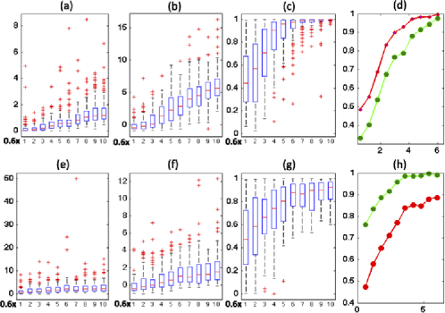
Inspecting Figure 1 reveals some findings as follows. First, deleting the $n$th cluster with 10 observations causes a larger effect than that with 1 observation [Figure 1(a) and (e), (d) and (h)]. As expected, the distributions of $\operatorname{CD}(\{n\})$ and $\widetilde{\operatorname{CSCD}}_{1}(I,\mathbf{Z})$ shift up as $b_{n}$ increases [Figure 1(a), (b), (e) and (f)]. Second, in the first scenario, $\operatorname{CD}(\{n\})$ is stochastically smaller than most other $\operatorname{CD}(I)$s, when the value of $b_{n}$ is relatively small [Figure 1(d)]. However, in the second scenario, $\operatorname{CD}(\{n\})$ is stochastically larger than most other $\operatorname{CD}(I)$s [Figure 1(h)] even for small values of $b_{n}$. Specifically, when $m_{n}=1$, the average $P_{C}(\{n\},\mathbf{Z})$ is smaller than 0.4 as $b_{n}=0.6$ and $b_{n}=1.2$, whereas when $m_{n}=10$, the average $P_{C}(\{n\},\mathbf{Z})$ is higher than 0.75 even as $b_{n}=0.6$. In contrast, in the two scenarios, the value of $P_{B}(\{n\},\mathbf{Z})$ is close to 0.5 as $b_{n}=0.6$ [Figure 1(d) and (h)]. It indicates that the cluster size does not have a big effect on the distribution of $\widetilde{\operatorname{CSCD}}_{1}(I,\mathbf{Z})$ [Figure 1(c) and (g)].

3.2 Yale infant growth data

The Yale infant growth data were collected to study whether cocaine exposure during pregnancy may lead to the maltreatment of infants after birth, such as physical and sexual abuse. A total of $298$ children were recruited from two subject groups (cocaine exposed group and unexposed group). One feature of this dataset is that the number of observations per children $m_{i}$ varies significantly from $2$ to $30$ Wasserman-Leventhal1993 , Stier-etal1993 . The total number of data points is $\sum_{i=1}^{n}m_{i}=3176$. Following Zhang Zhang1999 , we considered two linear mixed models given by $y_{i,j}=\mathbf{x}_{i,j}^{T}{{\bolds{\beta}}}+\varepsilon_{i,j},$ where $y_{i,j}$ is the weight (in kilograms) of the $j$th visit from the $i$th subject, $\mathbf{x}_{i,j}=(1,d_{i,j},(d_{i,j}-120)^{+},(d_{i,j}-200)^{+},(g_{i}-28)^{+},d_{i,j}(g_{i}-28)^{+},(d_{i,j}-60)^{+}(g_{i}-28)^{+},(d_{i,j}-490)^{+}(g_{i}-28)^{+},s_{i}d_{i,j},s_{i}(d_{i,j}-120)^{+})^{T}$, in which $d_{i,j}$ and $g_{i}$ (days) are the age of visit and gestational age, respectively, and $s_{i}$ is the indicator for gender. In addition, we assumed ${\bolds{\varepsilon}}_{i}=(\varepsilon_{i,1},\ldots,\varepsilon_{i,m_{i}})^{T}\sim N_{m_{i}}(\mathbf{0},R_{i}({\bolds{\alpha}}))$, where ${\bolds{\alpha}}$ is a vector of unknown parameters in $R_{i}({\bolds{\alpha}})$. We first considered $R_{i}({\bolds{\alpha}})=\alpha_{0}\mathbf{I}_{m_{i}}+\alpha_{1}\mathbf{1}_{m_{i}}^{\otimes 2}$. We refer to this model as model $M_{1}$. Then, it is assumed that variance and autocorrelation parameters are, respectively, given by $V(d)=\exp(\alpha_{0}+\alpha_{1}d+\alpha_{2}d^{2}+\alpha_{3}d^{3})$ and $\rho(l)=\alpha_{4}+\alpha_{5}l$, where $l$ is the lag between two visits. We refer to this model as model $M_{2}$.

Figure 2: Yale infant growth data. Panel (a) presents the line plot of infant weight against age, in which the observations of subject 269 are highlighted; panel (b) shows the cumulative residual curve versus age, in which the observed cumulative residual curve is highlighted in blue; and panels (c) and (d), respectively, present age versus raw residual and age versus standardized residual for cluster deletion.

We systematically examined the key assumptions of models $M_{1}$ and $M_{2}$ as follows.

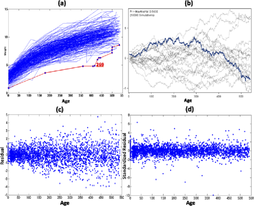
(i) We presented a cumulative residual plot and calculated the cumulative sums of residuals over the age of the visit to test $E[y_{i,j}|\mathbf{x}_{i,j}]=\mathbf{x}_{i,j}^{T}{{\bolds{\beta}}}$ Lin2002 , whose $p$-value is greater than 0.543. It may suggest that the mean structure is reasonable. The cumulative residual plot is given in Figure 2(b).

(ii) For model $M_{1}$, inspecting the plot of raw residuals $r_{i,j}=y_{i,j}-\mathbf{x}_{i,j}^{T}\hat{{\bolds{\beta}}}$ against age in Figure 2(c) reveals that the variance of the raw residuals appears to increase with the age of visit. As pointed by Zhang Zhang1999 , it may be more sensible to use model $M_{2}$. Let $\tilde{\mathbf{r}}_{i}=(\tilde{r}_{i,1},\ldots,\tilde{r}_{i,m_{i}})^{T}=R_{i}(\hat{{\bolds{\alpha}}})^{-1/2}\mathbf{r}_{i}$ be the vector of standardized residuals of $M_{2}$, where $\mathbf{r}_{i}=(r_{i,1},\ldots,r_{i,m_{i}})^{T}$. The standardized residuals under $M_{2}$ do not have any apparent structure as age increases [Figure 2(d)].

(iii) Under each model, we calculated $\operatorname{CD}(I)$ for each child Banerjee-Frees1997 . We treated ${{\bolds{\beta}}}$ as parameters of interest and all elements of ${\bolds{\alpha}}$ as nuisance parameters. For model $M_{1}$, we obtained a strong Pearson correlation of 0.363 between Cook’s distance and the cluster size. This indicates that the bigger the cluster size, the larger the Cook’s distance measure. Figure 4(b) highlights the top ten influential subjects. Compared with model $M_{1}$, we observed similar findings by using $\operatorname{CD}(I)$ under model $M_{2}$, which were omitted for space limitations.

There are several difficulties in using Cook’s distance under both models $M_{1}$ and $M_{2}$ Preisser-Qaqish1996 , Christensen-etal92 , Banerjee-Frees1997 , Banerjee1998 . First, cluster size varies significantly across children, and deleting a larger cluster may have a higher probability of having a larger influence as discussed in Section 2.3. For instance, we observe $(m_{285},\operatorname{CD}(\{285\}))=(8,0.738)$ and $(m_{274},\operatorname{CD}(\{274\}))=(22,1.163)$. A larger $\operatorname{CD}(\{274\})$ can be caused by a larger $m_{274}=22$ and/or influential subject 274, among others. Since $m_{274}$ is much larger than $m_{285}$, it is difficult to claim that subject $274$ is more influential than subject ${285}$. Second, there is no rule for determining whether a specific subject is influential relative to the fitted model. Specifically, it is unclear whether the subjects with larger $\operatorname{CD}(\{i\})$ are truly influential or not. Third, inspecting Cook’s distance solely does not seem to delineate the potential misspecification of the covariance structure under model $M_{1}$. We will address these three difficulties by using the new case-deletion measures.

Figure 3: Yale infant growth data. Panel (a) shows $m_{i}$ versus ${\mathcal{P}}(I|{\mathcal{M}}_{1})$, in which the ten subjects with the largest values of degree of perturbation or cluster size are highlighted; panel (b) shows ${\mathcal{P}}(I|{\mathcal{M}}_{1})$ versus $\operatorname{CD}(I)$, in which the top ten influential subjects are highlighted; panel (c) shows ${\mathcal{P}}(I|{\mathcal{M}}_{1})$ versus $\operatorname{CSCD}_{1}(I,\mathbf{Z})$, in which the top eleven influential subjects are highlighted; and panels (d), (e) and (f), respectively, show ${\mathcal{P}}(I|{\mathcal{M}})$, $\operatorname{CSCD}_{1}(I,\mathbf{Z})$ and $P_{B}(I,\mathbf{Z})$ for models ${\mathcal{M}}_{1}$ and ${\mathcal{M}}_{2}$.

(iv) Under each model, we calculated ${\mathcal{P}}(\{i\}|{\mathcal{M}})$ for deleting each subject $\{i\}$ for fixed covariates, and then we calculated the conditionally scaled Cook’s distances and associated quantities. We then used 1000 bootstrap samples to approximate ${\operatorname{CSCD}}_{1}(I,\mathbf{Z})$ and ${\operatorname{CSCD}}_{2}(I,\mathbf{Z})$. Subsequently, we calculated $P_{A}(I,\mathbf{Z})$ and $P_{B}(I,\mathbf{Z})$ in (15).

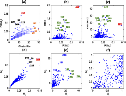
We observed several findings. First, under model $M_{1}$, we observed a strong positive correlation between ${\mathcal{P}}(\{i\}|{\mathcal{M}})$ and $m_{i}$ [Figure 3(a)]. Second, even though $m_{269}=12$ is moderate, subject $269$ has the largest degree of perturbation. Inspecting the raw data in Figure 2(a) reveals that subject 269 is of older age during visits compared with other subjects. Third, we also observed a strong positive correlation between ${\mathcal{P}}(\{i\}|{\mathcal{M}})$ and Cook’s distance [Figure 3(b)], which may indicate their stochastic relationship as discussed in Section 2.3. Fourth, we observed a positive correlation between Cook’s distance and the conditionally scaled Cook’s distance [Figure 3(b) and (c)], but their levels of influence for the same subject are quite different. For instance, the magnitude of $\operatorname{CSCD}_{1}(\{269\},\mathbf{Z})$ is only moderate, whereas $\operatorname{CD}_{1}(\{269\},\mathbf{Z})$ is the highest one. We observed similar findings under model ${\mathcal{M}}_{2}$ and presented some findings in Figure 3(d) and (e).

We used $P_{B}(I,\mathbf{Z})$ to quantify whether a specific subject is influential relative to the fitted model ${\mathcal{M}}_{1}$ [Figure 3(f)]. For instance, since $\operatorname{CD}(\{246\})=0.253$, it is unclear whether subject 246 is influential or not according to $\operatorname{CD}$, whereas we have $\operatorname{CSCD}_{1}(\{246\},\mathbf{Z})=21.443$ and $P_{B}(\{246\},\mathbf{Z})=1.0$. Thus, subject 246 is really influential after eliminating the effect of the cluster size. Moreover, it is difficult to compare the influential levels of subjects $274$ and $285$ using $\operatorname{CD}$. All of the conditionally scaled Cook’s distances and associated quantities suggest that subject $274$ is more influential than subject $285$ after eliminating the degree of perturbation difference. We observed similar findings under model ${\mathcal{M}}_{2}$ and omitted them due to space limitations. See Figure 3(d) and (e) for details.

We compared the goodness of fit of models ${\mathcal{M}}_{1}$ and ${\mathcal{M}}_{2}$ to the data by using the proposed case-deletion measures. First, inspecting Figure 3(d) reveals a strong similarity between the degrees of perturbation under models ${\mathcal{M}}_{1}$ and ${\mathcal{M}}_{2}$ for all subjects. Second, by using the conditionally scaled Cook’s distance, we observed different levels of influence for the same subject under ${\mathcal{M}}_{1}$ and ${\mathcal{M}}_{2}$. For instance, $\operatorname{CSCD}_{1}(I,\mathbf{Z})$ identifies subjects $246,141,109,193$ and $31$ as the top five influential subjects under ${\mathcal{M}}_{1}$, whereas it identifies subjects $274,217,90,109$ and $289$ as the top ones under ${\mathcal{M}}_{2}$. Finally, examining $P_{B}(I,\mathbf{Z})$ reveals a large percentage of influential points for model ${\mathcal{M}}_{1}$, but a small percentage of influential points for model ${\mathcal{M}}_{2}$; see Figure 3(f) for details. This may indicate that model ${\mathcal{M}}_{2}$ outperforms model ${\mathcal{M}}_{1}$. Furthermore, although we may develop goodness-of-fit statistics based on the scaled Cook’s distances and show that model ${\mathcal{M}}_{2}$ outperforms model ${\mathcal{M}}_{1}$, this will be a topic of our future research.

In summary, the use of the new case-deletion measures provides new insights in real data analysis. First, ${\mathcal{P}}(I|{\mathcal{M}})$ explicitly quantifies the degree of perturbation introduced by deleting each subject. Second, $\operatorname{CSCD}_{k}(I,\mathbf{Z})$ for $k=1,2$ explicitly account for the degree of perturbation for each subject. Third, $P_{B}(I,\mathbf{Z})$ allows us to quantify whether a specific subject is influential relative to the fitted model. Fourth, inspecting $P_{B}(I,\mathbf{Z})$ and $\operatorname{CSCD}_{k}(I,\mathbf{Z})$ may delineate the potential misspecification of the covariance structure under model $M_{1}$.

4 Discussion

We have introduced a new quantity to quantify the degree of perturbation and examined its properties. We have used stochastic ordering to quantify the relationship between the degree of the perturbation and the magnitude of Cook’s distance. We have developed several scaled Cook’s distances to address the fundamental issue of deletion diagnostics in general parametric models. We have shown that the scaled Cook’s distances provide important information about the relative influential level of each subset. Future work includes developing goodness-of-fit statistics based on the scaled Cook’s distances, developing Bayesian analogs to the scaled Cook’s distances, and developing user-friendly R code for implementing our proposed measures in various models, such as survival models and models with missing covariate data.

Appendix

The following assumptions are needed to facilitate the technical details, although they are not the weakest possible conditions. Because we develop all results for general parametric models, we only assume several high-level assumptions as follows.

Assumption A2.

$\hat{{{\bolds{\theta}}}}_{[I]}$ for any $I$ is a consistent estimate of ${{\bolds{\theta}}}_{*}\in\Theta$.

Assumption A3.

All $p(\mathbf{Y}_{[I]}|{{\bolds{\theta}}})$ are three times continuously differentiable on $\Theta$ and satisfy

$$\log p\bigl{(}\mathbf{Y}_{[I]}|{{\bolds{\theta}}}\bigr{)} = \log p\bigl{(}\mathbf{Y}_{[I]}|{{\bolds{\theta}}}_{*}\bigr{)}+\Delta({{\bolds{\theta}}})^{T}J_{n,{[I]}}({{\bolds{\theta}}}_{*})$$

$${}-0.5\Delta({{\bolds{\theta}}})^{T}\mathbf{F}_{n,{[I]}}({{\bolds{\theta}}}_{*})\Delta({{\bolds{\theta}}})+R_{[I]}({{\bolds{\theta}}}),$$

in which $|R_{[I]}({{\bolds{\theta}}})|=o_{p}(1)$ uniformly for all ${{\bolds{\theta}}}\in B({{\bolds{\theta}}}_{*},\delta_{0}n^{-1/2})=\{{{\bolds{\theta}}}\dvtx\sqrt{n}\|{{\bolds{\theta}}}-{{\bolds{\theta}}}_{*}\|\leq\delta_{0}\}$, where $\Delta({{\bolds{\theta}}})={{\bolds{\theta}}}-{{\bolds{\theta}}}_{*}$, $J_{n,{[I]}}({{\bolds{\theta}}})=\partial_{\theta}\log p(\mathbf{Y}_{[I]}|{{\bolds{\theta}}})$ and $\mathbf{F}_{n,{[I]}}({{\bolds{\theta}}}_{*})=\partial_{\theta}^{2}\log p(\mathbf{Y}_{[I]}|{{\bolds{\theta}}})$.

Assumption A4.

For any $I$ and $\mathbf{Z}$, $\sup_{\theta\in B({\theta}_{*},n^{-1/2}\delta_{0})}n^{-1/2}J_{n,{[I]}}({{\bolds{\theta}}})=O_{p}(1),$

$$\sup_{\theta\in B({\theta}_{*},n^{-1/2}\delta_{0})}\bigl{\|}\mathbf{F}_{n,[I]}({{\bolds{\theta}}})-E[\mathbf{F}_{I}({{\bolds{\theta}}})|{\mathcal{M}},\mathbf{Z}]\bigr{\|} = O_{p}\bigl{(}\sqrt{n}\bigr{)},$$

$$\sup_{\theta,\theta^{\prime}\in B({\theta}_{*},n^{-1/2}\delta_{0})}n^{-1}\bigl{\|}\mathbf{F}_{n,[I]}({{\bolds{\theta}}})-\mathbf{F}_{n,[I]}({\bolds{\theta}}^{\prime})\bigr{\|} = o_{p}(1),$$

and $0<\inf_{\theta\in B({\theta}_{*},\delta_{0}n^{-1/2})}\lambda_{\min}(n^{-1}\mathbf{F}_{n,[I]}({{\bolds{\theta}}}))\leq\sup_{\theta\in B({\theta}_{*},\delta_{0}n^{-1/2})}\lambda_{\max}(n^{-1}\times\mathbf{F}_{n,[I]}({{\bolds{\theta}}}))<\infty.$

Assumption A5.

For any set $I$ and $\mathbf{Z}$,

$$\sup_{\theta\in B({\theta}_{*},n^{-1/2}\delta_{0})}J_{{I}}({{\bolds{\theta}}}) = O_{p}\bigl{(}\sqrt{n(I)}\bigr{)},$$

$$\sup_{\theta\in B({\theta}_{*},n^{-1/2}\delta_{0})}\|\mathbf{f}_{I}({{\bolds{\theta}}})\| = O_{p}(n(I)),$$

$$\sup_{\theta\in B({\theta}_{*},n^{-1/2}\delta_{0})}\|\mathbf{f}_{I}({{\bolds{\theta}}})-E[\mathbf{f}_{I}({{\bolds{\theta}}})|{\mathcal{M}},\mathbf{Z}]\| = O_{p}\bigl{(}\sqrt{n(I)}\bigr{)}.$$

Assumptions A2–A5 are very general conditions and are generalizations of some higher level conditions for the extremum estimator, such as the maximum likelihood estimate, given in Andrews Andrews1999 . Assumption A2 assumes that the parameter estimates with and without deleting the observations in the subset $I$ are consistent. Assumption A3 assumes that the log-likelihood functions for any $I$ and $\mathbf{Y}_{[I]}$ admit a second-order Taylor’s series expansion in a small neighborhood of ${{\bolds{\theta}}}_{*}$. Assumptions A4 and A5 are standard assumptions to ensure that the first- and second-order derivatives of $p(\mathbf{Y}_{[I]}|{{\bolds{\theta}}})$ and $p(\mathbf{Y}_{I}|\mathbf{Y}_{[I]},{{\bolds{\theta}}})$ have appropriate rates of $n$ and $n_{I}$ Andrews1999 , Zhu-Zhang2006 . Sufficient conditions of Assumptions A2–A5 have been extensively discussed in the literature Andrews1999 , Zhu-Zhang2006 .

Proof of Theorem 1 (P.a) directly follows from the Jensen inequality, (6) and (7). For (P.b), if $I$ is an empty set, then $\operatorname{KL}(\mathbf{Y},{{\bolds{\theta}}}|I)\equiv 0$ and thus ${\mathcal{P}}(I|{\mathcal{M}})=0$. On the other hand, if ${\mathcal{P}}(I|{\mathcal{M}})=0$, then $\operatorname{KL}(\mathbf{Y},{{\bolds{\theta}}}|I)\equiv 0$ for almost every ${\bolds{\theta}}$. Thus, by using the Jensen inequality, we have $p(\mathbf{Y}_{I}|\mathbf{Y}_{[I]},\allowbreak{{\bolds{\theta}}})\equiv p(\mathbf{Y}_{I}|\mathbf{Y}_{[I]},{{\bolds{\theta}}}_{*})$ for all ${\bolds{\theta}}\in\Theta$. Based on the identifiability condition, we know that $I$ must be an empty set. Let $I_{1\cdot 2}=I_{1}-I_{2}$. It is easy to show that

$$p\bigl{(}\mathbf{Y}_{I_{1}}|\mathbf{Y}_{[I_{1}]},{{\bolds{\theta}}}\bigr{)}=p\bigl{(}\mathbf{Y}_{I_{2}},\mathbf{Y}_{I_{1\cdot 2}}|\mathbf{Y}_{[I_{1}]},{{\bolds{\theta}}}\bigr{)}=p\bigl{(}\mathbf{Y}_{I_{2}}|\mathbf{Y}_{[I_{2}]},{{\bolds{\theta}}}\bigr{)}p\bigl{(}\mathbf{Y}_{[I_{2}]}|\mathbf{Y}_{[I_{1}]},{{\bolds{\theta}}}\bigr{)}.$$

Thus, by substituting the above equation into (6), we have

$${\mathcal{P}}(I_{1}|{\mathcal{M}}) = {\mathcal{P}}(I_{2}|{\mathcal{M}})$$

$${}+\int p({{\bolds{\theta}}}|{{\bolds{\theta}}}_{*},\Sigma_{n*})p(\mathbf{Y}|{{\bolds{\theta}}})\log\biggl{(}\frac{p(\mathbf{Y}_{[I_{2}]}|\mathbf{Y}_{[I_{1}]},{{\bolds{\theta}}})}{p(\mathbf{Y}_{[I_{2}]}|\mathbf{Y}_{[I_{1}]},{{\bolds{\theta}}}_{*})}\biggr{)}\,d{{\bolds{\theta}}}\,d\mathbf{Y},$$

in which the second term on the right-hand side can be written as

$$\int p({{\bolds{\theta}}}|{{\bolds{\theta}}}_{*},\Sigma_{n*})p\bigl{(}\mathbf{Y}_{I_{2}}|\mathbf{Y}_{[I_{2}]},{{\bolds{\theta}}}\bigr{)}$$

$$\qquad{}\times\biggl{\{}\int p\bigl{(}\mathbf{Y}_{[I_{2}]}|{{\bolds{\theta}}}\bigr{)}\log\biggl{(}\frac{p(\mathbf{Y}_{[I_{2}]}|\mathbf{Y}_{[I_{1}]},{{\bolds{\theta}}})}{p(\mathbf{Y}_{[I_{2}]}|\mathbf{Y}_{[I_{1}]},{{\bolds{\theta}}}_{*})}\biggr{)}\,d\mathbf{Y}_{[I_{2}]}\biggr{\}}\,d{{\bolds{\theta}}}\,d\mathbf{Y}_{I_{2}}\geq 0,$$

which yields (P.c). Based on the assumption of (P.d), we know that

$$p\bigl{(}\mathbf{Y}_{[I_{2}]}|\mathbf{Y}_{[I_{1}]},{{\bolds{\theta}}}\bigr{)}=p\bigl{(}\mathbf{Y}_{I_{1\cdot 2}}|\mathbf{Y}_{[I_{1}]},{{\bolds{\theta}}}\bigr{)}=p\bigl{(}\mathbf{Y}_{I_{1\cdot 2}}|\mathbf{Y}_{[I_{1\cdot 2}]},{{\bolds{\theta}}}\bigr{)}$$

for all ${\bolds{\theta}}$. Thus, the second term on the right-hand side of (Appendix) reduces to ${\mathcal{P}}(I_{1\cdot 2}|{\mathcal{M}})$, which finishes the proof of (P.d).

Proof of Theorem 2 (a) Let $I_{3}=I_{1}\setminus I_{2}$, $I_{1}$ is a union of two disjoint sets $I_{3}$ and $I_{2}$. Without loss of generality, $H_{I_{1}}$ can be decomposed as

$$H_{I_{1}}=\mathbf{X}_{I_{1}}(\mathbf{X}^{T}\mathbf{X})^{-1}\mathbf{X}_{I_{1}}^{T}=\pmatrix{\mathbf{X}_{I_{2}}(\mathbf{X}^{T}\mathbf{X})^{-1}\mathbf{X}_{I_{2}}^{T}&\mathbf{X}_{I_{2}}(\mathbf{X}^{T}\mathbf{X})^{-1}\mathbf{X}_{I_{3}}^{T}\vspace*{2pt}\cr\mathbf{X}_{I_{3}}(\mathbf{X}^{T}\mathbf{X})^{-1}\mathbf{X}_{I_{2}}^{T}&\mathbf{X}_{I_{3}}(\mathbf{X}^{T}\mathbf{X})^{-1}\mathbf{X}_{I_{3}}^{T}}.$$

Let $\lambda_{1,1}\geq\cdots\geq\lambda_{1,n(I_{1})}\geq 0$ and $\lambda_{2,1}\geq\cdots\geq\lambda_{2,n(I_{2})}\geq 0$ be the ordered eigenvalues of $H_{I_{1}}$ and $H_{I_{2}}$, respectively, where $n(I_{k})$ denotes the number of observations in $I_{k}$ for $k=1,2$. It follows from Wielandt’s eigenvalue inequality Eaton-Tyler1991 that $\lambda_{1,l}\geq\lambda_{2,l}$ for all $l=1,\ldots,n(I_{2})$. For $k=1,2$, we define $\Gamma_{k}\Lambda_{k}\Gamma_{k}^{T}$ as the spectral decomposition of $H_{I_{k}}$ and $\mathbf{h}_{k}=(\mathbf{I}_{n(I_{k})}-\Lambda_{k})^{-1/2}\Gamma_{k}^{T}\hat{\mathbf{e}}_{I_{k}}=(h_{k,1},\ldots,h_{k,n(I_{k})})^{T}$, where $\Gamma_{k}$ is an orthnormal matrix and $\Lambda_{k}=\operatorname{diag}(\lambda_{k,1},\ldots,\lambda_{k,n(I_{k})})$. It can be shown that for $k=1,2$,

$$\mathbf{h}_{k}\sim N\bigl{(}\mathbf{0},\sigma^{2}\mathbf{I}_{n(I_{k})}\bigr{)}\quad\mbox{and}\quad\operatorname{CD}(I_{k})=\frac{1}{\hat{\sigma}^{2}}\sum_{j=1}^{n(I_{k})}\frac{\lambda_{k,j}}{1-\lambda_{k,j}}h_{k,j}^{2}.$$

Since $f(x)=x/(1-x)$ is an increasing function of $x\in(0,1)$, this completes the proof of Theorem 2(a).

Note that $\operatorname{CD}(I)=({\hat{\sigma}^{2}})^{-1}\sum_{j=1}^{n(I)}{\lambda_{j}}{(1-\lambda_{j})}^{-1}h_{j}^{2},$ where the $\lambda_{j}$ are the eigenvalues of $H_{I}$ and $\mathbf{h}=(h_{1},\ldots,h_{n(I)})^{T}\sim N(\mathbf{0},\sigma^{2}\mathbf{I}_{n(I)})$. Moreover, the distribution of $\lambda$ is uniquely determined by $H_{I}$. Combining $\mathbf{h}\sim N(\mathbf{0},\sigma^{2}\mathbf{I}_{n(I)})$ with the assumptions of Theorem 2(b) yields that $\operatorname{CD}(I)$ and $\operatorname{CD}(I^{\prime})$ follow the same distribution when $n(I)=n(I^{\prime})$. Furthermore, we can always choose an $I_{2}^{\prime}$ such that $n(I_{2}^{\prime})=n(I_{2})$ and $I_{1}\subset I_{2}^{\prime}$. Following arguments in Theorem 2(a), we can then complete the proof of Theorem 2(b).

Proof of Theorem 3 (a) It follows from a Taylor series expansion and Assumption A3 that

$$\partial_{\theta}\log p\bigl{(}\mathbf{Y}_{[I]}|\hat{{\bolds{\theta}}}_{[I]}\bigr{)}=\mathbf{0}=\partial_{\theta}\log p\bigl{(}\mathbf{Y}_{[I]}|\hat{{\bolds{\theta}}}\bigr{)}+\partial_{\theta}^{2}\log p\bigl{(}\mathbf{Y}_{[I]}|\tilde{{\bolds{\theta}}}\bigr{)}\bigl{(}\hat{{\bolds{\theta}}}_{[I]}-\hat{{\bolds{\theta}}}\bigr{)},$$

where $\tilde{{\bolds{\theta}}}=t\hat{{\bolds{\theta}}}_{[I]}+(1-t)\hat{{\bolds{\theta}}}$ for $t\in[0,1]$. Combining this with Assumption A4 and the fact that $\partial_{\theta}\log p(\mathbf{Y}|\hat{{\bolds{\theta}}})=\partial_{\theta}\log p(\mathbf{Y}_{[I]}|\hat{{\bolds{\theta}}})+\partial_{\theta}\log p(\mathbf{Y}_{I}|\mathbf{Y}_{[I]},\hat{{\bolds{\theta}}})=\mathbf{0}$, we get

$$\hat{{\bolds{\theta}}}_{[I]}-\hat{{\bolds{\theta}}} = \bigl{[}-\partial_{\theta}^{2}\log p\bigl{(}\mathbf{Y}_{[I]}|\hat{{\bolds{\theta}}}\bigr{)}\bigr{]}^{-1}\partial_{\theta}\log p\bigl{(}\mathbf{Y}_{[I]}|\hat{{\bolds{\theta}}}\bigr{)}[1+o_{p}(1)]$$ (21)

$$= -\bigl{[}-\partial_{\theta}^{2}\log p\bigl{(}\mathbf{Y}_{[I]}|\hat{{\bolds{\theta}}}\bigr{)}\bigr{]}^{-1}\partial_{\theta}\log p\bigl{(}\mathbf{Y}_{I}|\mathbf{Y}_{[I]},\hat{{\bolds{\theta}}}\bigr{)}[1+o_{p}(1)].$$

Substituting (21) into $\operatorname{CD}(I)=(\hat{{\bolds{\theta}}}_{[I]}-\hat{{\bolds{\theta}}})^{T}\mathbf{F}_{n}(\hat{{\bolds{\theta}}})(\hat{{\bolds{\theta}}}_{[I]}-\hat{{\bolds{\theta}}})$ completes the proof of Theorem 3(a).

(b) It follows from Assumptions A2–A4 that

$$\hat{{\bolds{\theta}}}-{{\bolds{\theta}}}_{*} = \mathbf{F}_{n}({{\bolds{\theta}}}_{*})^{-1}\partial_{\theta}\log p(\mathbf{Y}|{{\bolds{\theta}}}_{*})[1+o_{p}(1)]$$

$$= \mathbf{F}_{n}({{\bolds{\theta}}}_{*})^{-1}\bigl{[}\partial_{\theta}\log p\bigl{(}\mathbf{Y}_{[I]}|{{\bolds{\theta}}}_{*}\bigr{)}+\partial_{\theta}\log p\bigl{(}\mathbf{Y}_{I}|\mathbf{Y}_{[I]},{{\bolds{\theta}}}_{*}\bigr{)}\bigr{]}[1+o_{p}(1)].$$

Let $J_{I}({{\bolds{\theta}}})=\partial_{\theta}\log p(\mathbf{Y}_{I}|\mathbf{Y}_{[I]},{{\bolds{\theta}}})$. Using a Taylor series expansion along with Assumptions A4 and A5, we get

$$J_{I}(\hat{{\bolds{\theta}}}) = J_{I}({{\bolds{\theta}}}_{*})-\mathbf{s}_{I}({{\bolds{\theta}}}_{*})(\hat{{\bolds{\theta}}}-{{\bolds{\theta}}}_{*})[1+o_{p}(1)]$$

$$= J_{I}({{\bolds{\theta}}}_{*})-E[\mathbf{s}_{I}({{\bolds{\theta}}}_{*})|{\mathcal{M}}](\hat{{\bolds{\theta}}}-{{\bolds{\theta}}}_{*})[1+o_{p}(1)]$$

$$= \bigl{(}\{\mathbf{I}_{p}-E[\mathbf{s}_{I}({{\bolds{\theta}}})|{\mathcal{M}}]\mathbf{F}_{n}({{\bolds{\theta}}}_{*})^{-1}\}J_{I}({{\bolds{\theta}}}_{*})$$

$${}-E[\mathbf{s}_{I}({{\bolds{\theta}}})|{\mathcal{M}}]\mathbf{F}_{n}({{\bolds{\theta}}}_{*})^{-1}\partial_{\theta}\log p\bigl{(}\mathbf{Y}_{[I]}|{{\bolds{\theta}}}_{*}\bigr{)}\bigr{)}[1+o_{p}(1)].$$

Since $E[J_{I}({{\bolds{\theta}}}_{*})\partial_{\theta}\log p(\mathbf{Y}_{[I]}|{{\bolds{\theta}}}_{*})|{\mathcal{M}}]=\mathbf{0}$,

$$E[J_{I}(\hat{{\bolds{\theta}}})J_{I}(\hat{{\bolds{\theta}}})^{T}|{\mathcal{M}}]$$

$$\qquad=E[\mathbf{s}_{I}({{\bolds{\theta}}}_{*})|{\mathcal{M}}]\mathbf{F}_{n}({{\bolds{\theta}}}_{*})^{-1}\{\mathbf{F}_{n}({{\bolds{\theta}}}_{*})-E[\mathbf{s}_{I}({{\bolds{\theta}}}_{*})|{\mathcal{M}}]\}[1+o_{p}(1)].$$

It follows from Assumption A4 that for ${\bolds{\theta}}$ in a neighborhood of ${{\bolds{\theta}}}_{*}$, $\mathbf{F}_{n}({{\bolds{\theta}}})$ and $\mathbf{F}_{n}({{\bolds{\theta}}}_{*})-\mathbf{f}_{I}({{\bolds{\theta}}})$ can be replaced by $E[\mathbf{F}_{n}({{\bolds{\theta}}})|{\mathcal{M}}]$ and $E[\mathbf{F}_{n}({{\bolds{\theta}}}_{*})-\mathbf{f}_{I}({{\bolds{\theta}}})|{\mathcal{M}}]$, respectively, which completes the proof of Theorem 3(b).

(c) Similarly to Theorem 3(b), we can prove Theorem 3(c).

[id=suppA] Supplement to “Perturbation and scaled Cook’s distance” [doi,text=10.1214/12-AOS978SUPP]10.1214/12-AOS978SUPP .pdf aos978_supp.pdf We include two theoretical examples and additional results obtained from the Monte Carlo simulation studies and real data analysis. ().