Resummed Perturbation Theory of Galaxy Clustering
Abstract
The relationship between observed tracers such as galaxies and the underlying dark matter distribution is crucial in extracting cosmological information. As the linear bias model breaks down at quasi-linear scales, the standard perturbative approach of the nonlinear Eulerian bias model (EBM) is not accurate enough in describing galaxy clustering. In this paper, we discuss such a model in the context of resummed perturbation theory, and further generalize it to incorporate the subsequent gravitational evolution by combining with a Lagrangian description of galaxies’ motion. The multipoint propagators we constructed for such model also exhibit exponential damping similar to their dark matter counterparts, therefore the convergence property of statistics built upon these quantities is improved. This is achieved by applying both Eulerian and Lagrangian resummation techniques of dark matter field developed in recent years. As inherited from the Lagrangian description of galaxy density evolution, our approach automatically incorporates the non-locality induced by gravitational evolution after the formation of the tracer, and also allows us to include a continuous galaxy formation history by temporally weighted-averaging relevant quantities with the galaxy formation rate.
I Introduction
Large-scale structure surveys provide a wealth of cosmological information in probing dark energy, modified gravity, neutrino masses and the physics of early universe. As the statistical uncertainty decreases dramatically in next generation surveys, it requires us to achieve an unprecedented level of accuracy in theoretically predicting the statistics of the observed clustering pattern. Since nonlinear dynamics plays a important role in understanding the observed data in relevant regime, it has attracted lots of interest in developing the nonlinear perturbation theory of the dark matter beyond the standard approach. Many sophisticated methods have been proposed, including the renormalized perturbation theory (RPT) (Crocce & Scoccimarro, 2006a, b; Bernardeau et al., 2008), the Lagrangian resummation theory (Matsubara, 2008a), the closure theory (Taruya & Hiramatsu, 2008), and the time renormalization group theory (TRG) (Pietroni, 2008). However, the relationship between various observable tracers (galaxies, quasars, Ly forest, clusters and HI galaxies etc.) and the underlying dark matter field may be more challenging. The linear bias model breaks down even for present surveys (Sanchez & Cole, 2008; Percival et al., 2007) at relatively large scale, the scale-dependence observed in the data varies among different galaxy samples as one would expect (Sanchez & Cole, 2008), and the empirical fitting formula (Coles et al., 2005) widely used in the data analysis is not able to describe such differences among samples and eventually leads to inconsistent cosmological constraints (Sanchez & Cole, 2008).
Two different approaches exist in modeling the scale-dependent bias of galaxies these days. One is the halo-based model which starts from the large scale clustering of dark matter halos and then populates with different types of galaxies according to the halo occupation distribution (HOD) function. The other approach is the perturbative bias model, which packs the complicated baryonic physics into a general unknown functional depending on the dark matter distribution, and characterize it with the first few bias parameters. With a careful parameterized and calibrated HOD function, the first approach can describe the two-point statistics qualitatively well at small scale. However, a viable HOD parameterization usually contains lots of free parameters, and heavily depends on calibration from simulation. Moreover, in the quasi-linear regime where most of large-scale surveys probe, the accuracy of such approach is usually not satisfactory.
On the other hand, the standard perturbative bias model is also problematic. In the Eulerian bias model (EBM), the observed galaxy number density depends on the Eulerian dark matter distribution at the time of observation. Therefore, this model breaks down as the dark matter perturbations evolve into the nonlinear regime at small scales and later times. Since both the large-scale amplitude and small-scale shape of the power spectrum depend on higher-order bias parameters, such calculation would fail within the whole range of scales. Furthermore, although adopting some artificial nonlocal bias parameters won’t bring too much intrinsic difficulties in the calculation, most authors simply assume that the functional form of the galaxy density only depends on the matter distribution locally, which is not consistent with the nonlocal gravitational evolution of the tracer (Matsubara, 2011; Chan et al., 2012).
Since the difficulties of the perturbative convergence encountered in the nonlinear bias model is very similar to the situation in dark matter field, one would expect to generalize any of previous nonstandard matter perturbation theory to describe the clustering of biased tracer. Several works have already been done along this direction. In Matsubara (2008b), a Lagrangian bias model (LBM) which intended to incorporate the halo bias and redshift distortion was proposed based on a similar resummation theory for matter distribution (Matsubara, 2008a). Then Elia et al. (2011) also included the halo bias in the time renormalization group methods. McDonald (2006, 2009) approached in a different way by redefining the bias parameters. As we will show in this paper, with the help of recent development in the renormalized perturbation theory Crocce & Scoccimarro (2006a, b); Bernardeau et al. (2008), it is also possible to construct a resummed perturbation theory for nonlinear Eulerian bias model, and the perturbative expansion of statistics can be rewritten through the so-called expansion, first introduced by Bernardeau et al. (2008), with the building blocks known as multipoint propagators. One advantage of the expansion is that for Gaussian initial conditions, all contributions are positive and centralized within a limited range of scale. As we will see later, such an expansion is quite general and applicable to many circumstances as long as the multipoint propagators can be well estimated. Therefore in the following, this paper will mainly concentrate on constructing the multipoint propagators for various objects. The validity of such technique has already been verified in calculating the power spectrum of logarithmic mapping of the density field Wang et al. (2011). It have been shown that even for the slow converging function such as logarithm, the calculation agrees with the simulation quite well.
We further generalize the Eulerian bias model by separating the complicated nonlinear physical processes during the galaxy formation and the subsequent gravitational evolution until been observed by a survey. As we will show, this can be achieved by combining the Eulerian bias model and Lagrangian description of galaxy motion introduced in Matsubara (2008b). Like EBM, we assume the galaxy distribution created at some time is characterized by a general unknown functional, and the galaxy number density observed at a Eulerian position later can be naturally described by the Lagrangian version of continuity equation. Consequently, this approach also enables us to incorporate continuous galaxy formation by temporally averaging the distribution of newborn galaxies weighted with the galaxy formation rate. In such a framework, while the complex galaxy formation physics is simplified by a few bias parameters, we are able to capture the following gravitational evolution after its creation, which would in principal induce non-locality and can not be accurately described by a local Eulerian bias model. As inherited from the Lagrangian bias model and our resumed calculation of Eulerian bias model, this model can also be expressed in a resummed manner.
In section II, we briefly review both Eulerian and Lagrangian perturbation theory of dark matter field, including both standard approach and resummed theory. We will also introduce the concept of the multipoint propagator in the context of Lagrangian perturbation theory, and give a explicit calculation in Appendix A. In section III, we first review the standard Eulerian and Lagrangian bias model, and then introduce our continuous galaxy formation model. We construct the resummed Eulerian bias model in Section IV, and the generalize it in Section V. Finally, we conclude in Section VI.
II Perturbation Theory of Dark Matter
In this section, we will briefly review both Eulerian perturbation theory (EPT) and the Lagrangian perturbation theory (LPT) of the dark matter field, including both the standard approach and resummed calculation.
II.1 Dynamical Equation of Motion
The gravitational dynamics of a pressureless fluid before shell crossing is governed by the continuity, Euler, and Poisson equations.
| (1) |
Here, is the Hubble expansion rate, is the scale factor, is the ratio of matter density to critical density, and is the Newtonian potential.
Following Crocce & Scoccimarro (2006a, b), the equation of motion in Fourier space can be written in a compact form by defining the two-component variable
| (2) |
where denotes the divergence of peculiar velocity . The index stands for matter density or velocity variables, respectively. In the following, we will interchangeably use , and for matter overdensity, while using both and for galaxy perturbation.
The equation of motion then reads
| (3) | |||||
with the convention that repeated Fourier arguments are integrated over. The time in a Einstein-de Sitter (EdS) universe. Here the constant matrix
| (6) |
derived for an EdS universe, is still applicable in other cosmologies with negligible corrections to the coefficients, using (with the linear growth factor).
The symmetrized vertex matrix is given by
| (7) |
, and otherwise.
Then the formal integral solution to Eq. (3) can be derived as
| (8) | |||||
where denotes the initial condition , and the linear propagator is given by
| (13) |
In the following, we adopt growing-mode initial conditions , with .
In Lagrangian perspective, the dynamic of a fluid element at initial Lagrangian position is entirely described by the final Eulerian position , or equivalently the displacement field , which is governed by the equation of motion,
| (14) |
where is still the derivative with respect to Eulerian coordinates , and the gravitational potential is determined by Poisson equation as shown in Eq. (II.1). The density contrast is then related to via mass conservation
| (15) |
where is the Jacobian of the transformation between Eulerian and Lagrangian space, and . To linear order, Eq. (14) is then solved by the Zel’dovich approximation , with Lagrangian derivative .
II.2 Eulerian Perturbation Theory
A perturbative solution to Eq. (8) could be obtained by expanding in terms of initial fields
| (16) | |||||
where is short for , and denotes . The kernels are fully symmetric functions of the wave vectors. As shown in Crocce & Scoccimarro (2006b), they can be obtained in terms of and recursively.
| (17) |
For , . It should be noted that in this formalism, the kernel depends on the time , since it includes subleading terms in (Crocce & Scoccimarro, 2006a). If one only considers the fastest-growing mode, equals the well-known PT kernel , where is the linear growth factor.

The power spectrum of the matter density perturbation is defined as
| (18) |
For Gaussian initial conditions, all the statistical information is encoded in the initial power spectrum
| (19) |
where , with . Diagrammatically, as shown in the right-hand diagram of Fig. (1), the ensemble average is obtained by gluing two open circles together to form the symbol , which represents the initial power spectrum .

As the density fluctuations evolve into the non-linear regime at later times, the validity of standard perturbation theory breaks down, loop contributions become ill-behaved and the convergence of perturbation series gets out of control. As one of several different approaches beyond SPT been proposed recently, we will briefly review the renormalized perturbation theory (RPT) introduced by Crocce & Scoccimarro (2006a, b); Bernardeau et al. (2008), and then the Lagrangian resummation theory (Matsubara, 2008a) in the next subsection.
The crucial step of renormalized perturbation theory is to define the generalized growth factor, known as the propagator
| (20) |
which effectively describes the time evolution of individual Fourier modes when non-linear mode-coupling is included. Here denotes the functional derivative. The propagator measures the dependence of a non-linearly evolved Fourier mode on its initial state on average. Intuitively, one should expect to decay to zero at small scales since non-linear mode-coupling has erased all the information from the initial state at that . Indeed, with the help of the Feynman diagrams introduced in Crocce & Scoccimarro (2006a), the dominant contribution can be summed up explicitly in the large-k limit, and giving the exponential decay . In this paper, the non-linear propagator is diagrammatically presented as a grey circle with an incoming branch. It is a summation of infinite number of loop contributions, as illustrated in Fig. (2).
Given above, Crocce & Scoccimarro (2006a) was able to rewrite the nonlinear matter density power spectrum as a sum of two contributions
| (21) |
where is the density propagator , and is the mode-coupling term. Therefore, the non-linear power spectrum at any is composed of two parts. One is proportional to the initial power spectrum at the same ; the other comes from mode-coupling of other . As decays at small scales, more and more power comes from the mode-coupling contribution. Bernardeau et al. (2008) showed that these complicated mode-coupling contributions can be expressed as a summation of multi-point propagators, defined as
| (22) |
which is nothing but a generalization of two-point propagator . Similarly, the dominant part of multi-point propagators can also be summed and decay into the nonlinear regime at the same rate as two-point propagator. Bernardeau et al. (2008) showed that a simple approximation which generalizes the -dependence of two-point propagators agrees with the data with acceptable accuracy,
| (23) | |||||
For gaussian initial condition, the nonlinear power spectrum can then be expressed with the help of Eq.(II.2), known as the expansion
| (24) | |||||
Note that Eq. (24) describes nothing but an alternative way of taking ensemble averages, or diagrammatic speaking, gluing initial states. Instead of gluing two density fields order by order, one can first construct the objects by gluing initial states of individual density fields with incoming branches, known as an ()-point propagator, and the final non-linear power spectrum is then obtained by gluing two propagators together. Therefore, this expansion is quite general and applicable to the ensemble average of any two arbitrary statistical fields , which are functionals of some other field
| (25) | |||||
as long as the building blocks are well estimated. Here symbolize some parameters, and are symmetric on their arguments. In the case that is Gaussian, the Wick’s theorem ensures that the ensemble average of an odd number of fields vanishes and the average of an even number of fields can be decomposed as summation of two-point correlations
| (26) |
Following the idea of Bernardeau et al. (2008), there are three types of two-point correlations involved in calculating : pairs within or themselves and pairs connecting them. Therefore, one is always able to regroup Eq.(26) in the following way
Combining above equations (25, 26 and II.2) together, one is able to reformulate as a sum of two-point cross correlations of belonging to and respectively with some pre-summed nonlinear quantity involving internal pairs , which can be formally defined as the average of functional derivative
| (28) |
Therefore, as long as is well estimated, one is always able to carry out the expansion in such situation. In the following, we will demonstrate that with the help of the density propagator of cold dark matter (Eq. II.2), many similar quantities of this kind can be calculated. And we will extensively utilize such expansion in the following of the paper.
II.3 Lagrangian Perturbation Theory
As discussed in the beginning of this section, the dynamics of the system in Lagrangian picture is fully characterized by the displacement field . Combining the equation of motion (Eq. 14) and the Poisson equation, the displacement field can be solved perturbatively. In Fourier space, the th order perturbation can be generally expressed as
where is the perturbation kernel.
Due to the matter conservation, the Eulerian density contrast can be expressed as
| (30) |
For the matter distribution, one usually assumes that the initial field is sufficiently uniform , so that above equation (Eq. 30) can be further simplified. In Fourier space,
| (31) | |||||
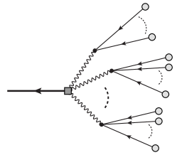
Similarly, the above equation can also be represented by diagrams as shown in Fig. (3). Here, wavy lines denote the displacement field , and the thin solid line together with grey open circle stands for the linear density perturbation, i.e. Eq.(II.3).
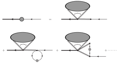
Starting from Eq.(31), Matsubara (2008a) performed a resummation of the power spectrum of the density contrast, known as Lagrangian Resummed Perturbation Theory. Although not been explicitly discussed in Matsubara (2008a), it is also possible to define the same propagator within this framework. First of all, as pointed out in Matsubara (2011) for biased tracers111Setting and otherwise in Eq. (71) of Matsubara (2011), one recovers the following equation., the following quantity can be resummed
| (32) |
where is the displacement field at the origin. It is represented as a grey ellipse in Fig. (4), and can be further simplified as Matsubara (2008a, 2011)
| (33) | |||||
with the variance of displacement field along one direction . Here, we have used the cumulant theorem
| (34) |
where denotes the connected part of the ensemble average. As shown in Matsubara (2011), it leads us to a partial resummation of the propagator as represented in Fig. (4) up to the one-loop order. Again, this is just a simplified version of Fig. (17) in Matsubara (2011) for the Lagrangian bias model. The grey ellipse represents all possible graphs attached with various number of wavy lines, i.e. Eq. (II.3). Compared to the diagram introduced in Matsubara (2011), we have omitted the summation sign over external wavy lines. Mathematically, such diagrammatical series is equivalent to
Note that we have used an alternative version of the cumulant theorem in Eq. (34).
| (36) |
which is obtained by taking the derivative of Eq. (34) respect to and then setting it to zero. We further calculate these contributions explicitly in the Appendix A. The result is not the same as the form originally proposed by Crocce & Scoccimarro (2006b). However, the matching prescription between high-k and one-loop calculation in Crocce & Scoccimarro (2006b) seems more or less ad hoc. Therefore, an alternative way of constructing the propagators was proposed by Bernardeau (2011), to which our calculation do agree. See Bernardeau (2011) for the discussion of different versions of calculating multipoint propagators.
III The Non-linear Bias Model
III.1 Eulerian Bias Model
In Eulerian bias model, the galaxy number density perturbation at time is considered as some general functional of the underlying matter density distribution characterized by its Taylor coefficient
| (37) |
where the nonlinear mass density field is solved by perturbation theory mentioned in the last section. As discussed by Matsubara (2011), this functional is generally non-local. Therefore in Fourier space, bias coefficient depends on wavenumbers
| (38) | |||||
In the local bias model, then becomes constant times a smoothing window function in Fourier space. In this model, the linear bias relation at large scale is not only attributed to the first term in Eq. (38), but also from the higher orders . As first pointed out by Scherrer & Weinberg (1998), the effective large scale bias is determined by infinite number of higher-point local variances of the field. Therefore, similar to the situation in the standard perturbation theory of matter density field, at later time when mass density variance grows larger, a naive perturbative expansion fails. In this case, such a breakdown affects both the large scale amplitude and the high-k regime of the power spectrum.
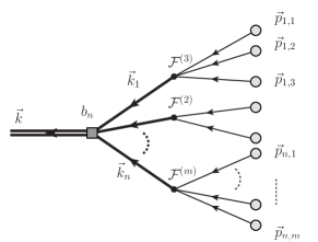
Given the definition of in Eq.(38) and the diagrammatic representation of the density perturbation in Fig. (1), it is also possible to draw diagrams representing . As depicted in Fig.(5), each diagram contains two levels of nonlinear interactions. The thick solid -branch tree represents the nonlinear convolution, and their interaction vertex, shown as a solid square, carries the bias coefficient , where is the number of branches. Each branch represents one nonlinearly evolved density contrast at time , which is followed by another thin branches, to express its gravitational nonlinearity in terms of initial fields and perturbative kernels . At the end of each branch, small open circles represent the initial conditions . When expanding to different orders, one should also include the information about the number of topologically equivalent diagrams, which essentially comes from the multinomial coefficient of . The final field is then a summation of all possible diagrams.
III.2 Lagrangian Bias Model
To incorporate the halo bias with nonlinear perturbation theory, Matsubara (2008b) proposed an alternative bias model involving the initial Lagrangian density fluctuation instead of final Eulerian density . In this Lagrangian bias model, the non-linear objects, typically halos, were formed at some initial time with the number density is a functional of underlying linear density distribution . Then the Eulerian observable at later time is described by the continuity relation
where is the displacement field of such tracer. In Fourier space,
| (40) |
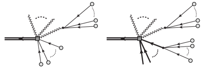
In the limits that nonlinear objects trace exactly the underlying dark matter, i.e. , one can further proceed to calculate the power spectrum using Lagrangian perturbation theory of the matter field. In Fig. (6), we reproduced the diagram of this model introduced by Matsubara (2011) on the left, where the wavy line represents the displacement field and the branches of thin solid lines with open circle symbolize the th order of .
The great advantage of this approach is that it naturally takes account of the non-locality induced by gravitational evolution. As shown by Matsubara (2011), after perturbatively expanding both sides of Eq.(40) and comparing terms order by order, one obtains the relationship between Eulerian and Lagrangian bias parameters. To the first two orders (Matsubara, 2011),
| (41) | |||||
Therefore, even if the Lagrangian bias is local initially, non-linear and non-local gravitational evolution would render the Eulerian bias non-local.
III.3 Continuous Galaxies Formation Model
As briefly mentioned in the introduction, we will try to generalize the Eulerian bias model in two different ways. As the resummation technique will be discussed in next two sections, in the following of this section, we will try to construct a model by combining Eulerian and Lagrangian pictures together.
First, we still assume that the complicated nonlinear process leading to the formation of galaxies or other type of observable tracers can be described by a general nonlinear functional at the moment of galaxy creation. In general this can be nonlocal, however, we will assume to be local for simplicity. As what will be seen in the following, the locality assumption here is not as problematic as in the local Eulerian bias model since it only relates to the physical process during the moment of galaxy formation and could be easier to generalize. Furthermore, such functional can also explicitly depends on the formation time, i.e. we have and .
Assuming at time , there are new galaxies were created during at a Lagrangian-like position , and then evolved to Eulerian position where have been observed by a survey at time . Analogous to the Lagrangian bias model (Eq. III.2), this contributes to the Eulerian galaxies a number density
| (42) |
where is the displacement field of galaxy from to . Note that here only comprises galaxies that are finally selected in the sample. Therefore, the galaxy number density at observed time and comoving position is a sum of all contributions that formed before and then moved to with a displacement ,
| (43) | |||||
Here we have written the number density , where is the nonlinear evolved matter density field at . In principle, the displacement field of galaxies should follow the one of dark matter , i.e.
| (44) |
where is some initial Lagrangian position of the matter field when density perturbation is still linear. In the following of this paper, we will assume . In the simplest case where all galaxies formed at , i.e. , a similar form of Eq.(III.2) is recovered. Taking the average of both sides of Eq.(43), one obtains the average number density as a integration of the average density over the whole galaxy formation history
| (45) |
Therefore, the perturbation of galaxy number density can then be expressed as,
| (46) | |||||
where denotes the average galaxies formation rate, with the normalization relation . To first order, we have
Therefore, the linear bias of galaxies evolves as
| (48) |
In the case that galaxies exactly trace cold dark matter, i.e. , we recover the result calculated by Chan et al. (2012) if only the growing mode is considered. As first discussed by Tegmark & Peebles (1998), for the model galaxies burst at a single time , ,
| (49) |
So the gravitational growth will always debias the clustering of galaxies towards .
Because of this Lagrangian-like approach adopted here, this framework automatically incorporates the gravitational non-locality induced after the formation of the galaxies. Furthermore, as will be seen in Section V., Eq. (46) also allows the application of the resummation technique so that the perturbative convergence of such model is guaranteed.
IV Resummed Perturbation Theory of Eulerian Bias Model
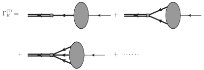
In this section, we will show that the Eulerian bias model can be partially resummed with the help of exponential decay of multipoint matter propagators . Starting from the definition of this model (Eq. 38), one can define the ()-point nonlinear propagator of the biased-tracer overdensity ,
| (50) |
Before substituting (Eq. 38) as well as the perturbative solution of (Eq. II.2, 24) into above definition, one first notices that, can be expanded in terms of the number of nonlinear density fields involved, just as depicted in the schematic diagram of Fig.(7) for the two-point propagator. Mathematically, it means , where
| (51) |
For the two-point propagator , let us write down all contributions formally. First of all, it is clear that the one- term, i.e. the first diagram in Fig.(7), equals the two-point propagator of the matter field itself multiplied with the linear bias parameter . For the two- contribution, i.e. the second diagram, one reads from Eq. (IV)
| (52) | |||||
As discussed in Section II, the ensemble average at the second line can be expanded by a like series, which in this case, is the propagator for matter field . To proceed, we expand Eq. (52) explicitly
| (53) | |||||
As we have shown, Wick’s theorem ensure the decomposition of joint ensemble average at the last line into the combinations of two-point correlations. Each of these terms can be labeled by three indices , where , , i.e. we classify all pairs into three categories: pairs within the first field ; pairs within the second field ; and pairs in between. The renormalization is then achieved by realizing that a pre-summation of and gives rise to one -point and another -point propagator, therefore
| (54) |
where we have introduced the notation
and used the definition of in terms of the perturbation kernel. The coefficient then comes from all possible ways of matching initial states with another group of initial states. For this contribution, the only difference between Eq.(IV) and Eq.(24) is the order of the matter propagator been summed. For the RPT description of the matter power spectrum, both propagators share the same order; otherwise, it would be impossible to match the pair. For the same reason, the order of one propagator in Eq.(IV) is always greater than the other by one, since we have to select one branch out before taking the average.
The formula can be further generalized to arbitrary order ,
where the index denotes the number of connections between the -th and the -th density field (e.g. for ), so the total number of the indices is then . The coefficient is then given by
| (57) | |||||
Here, is the total number of connections linked between the -th density field and others, with . Eq. (57) expresses the products of multinomial coefficients of choosing from for each density field, times all possible permutations within for pair matching. Each connection carries a momentum , which characterizes the -th connection between -th and -th . The integration is taken over momenta of all possible connections among different density fields. Because of the ensemble average Eq.(19), we have . , and we also used the shorthand notation for .
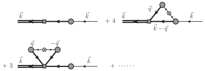
Given above expressions, we are then able to expand in terms of the number of initial power spectra entering the calculation. For the tree level, it simply reads as
| (58) |
where we have introduced the notation
| (59) |
where is some smoothing window function.
At one-loop level, from Eq.(IV), the contribution would be nonzero only when , since otherwise there would exist at least one with zeroth order, which would vanish because . For , , the coefficient equals . For , , the coefficient equals . So we have
| (60) |
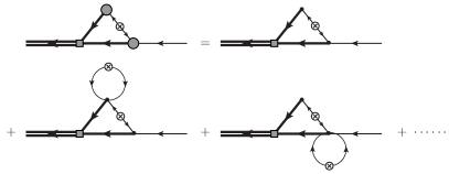
To make the Eq.(IV) easier to understand, one can draw every contribution diagrammatically. Starting from the diagram representing in Fig.(5), we change all kernels into -point propagators. After selecting one particular branch out, we glue the rest of the initial states (open circles) together. Every resultant topologically inequivalent diagram represents one or several terms in Eq.(IV). Since all ordinary kernels have already been substituted by propagators, the ensemble average (gluing) is only performed among different density fields . In Fig.(8), we show all diagrams of up to one-loop order. They correspond one-to-one to Eq.(58) and Eq.(IV). We also present all two-loop diagrams and equations of in Appendix B. It should be emphasized that, by substituting ordinary kernels into propagators, each diagram in fact contains an infinite number of loop contributions at every substituting position, as shown in Fig.(9).
Numerically, the Gaussian damping of the multipoint matter propagator will eventually contribute to the improvement of the convergence in calculating nonlinear matter power spectrum. Therefore, it is important to check whether share the similar feature. From diagrams representing , we see that there exists a straight path through the diagram carrying the same momentum at both the start and end. Along this path, there is one convolution bias vertex , as well as one -point propagator . For (e.g. the third diagram in Fig.(8)), this contribution recovers the same -dependence as , rescaled by a constant from loop integration. When , Eq.(23) suggests a similar damping of given . Meanwhile every propagator associates with a smoothing window function . Therefore one should expect that, in the large- limit, will decay as a combined effect of a Gaussian damping of and the smoothing window function.
Besides the tree level result of two-point propagator , which equals the one of dark matter field times the linear bias coefficient , the loop integration from higher-order calculation, e.g. the third diagram in Fig.(8), will also change the small- normalization of and eventually the effective large-scale bias of the power spectrum . As we will see at the end of this section, dominates the contribution of , hence the accuracy of the depends on the precision of estimating the . Due to the exponential decay of matter propagators , our resummed formula will help us in improving the convergence of .

Now, we can further derive the three-point propagator similarly, except that two distinct contributions have to be taken into account because of the second order functional derivative in the definition of .
| (61) | |||||
As shown in Eq.(61), the first term takes the joint average of the products of a second derivative with density fields. Diagrammatically speaking, it corresponds to selecting two branches from a single , i.e. the first diagram in Fig. (10). In Fig. (18) of Appendix C, this category includes the first, third and sixth diagram. The rest of the diagrams then correspond to the second term of Eq.(61), where two branches originate from two different density fields. Both terms can be written in the same form of Eq.(IV),
The difference between the two terms can be clearly seen from their orders of the matter propagators. With the same labeling system, the first gives , while the second gives . Meanwhile, the two coefficients equal
| (63) | |||||
The first contribution gives , while the second term gives .
At tree level, there are two diagrams: one is , from the single- contribution; and the other is the two- term with for the second term of Eq.(IV),
All the one-loop contributions can be found in the Appendix C.
Finally, the non-linear power spectrum of the field can be expressed as
| (65) | |||||
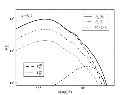


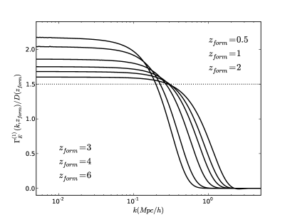
In Fig. (11), we illustrate the numerical calculation of the power spectrum of Eulerian bias model at redshift for bias parameters and , assuming a spherical top-hat smoothing length . The solid line gives the full nonlinear power spectrum of including both and contributions. Each of them is then represented by the long dashed and the short dashed line respectively. We only calculate the up to one-loop order while to the two-loop order. Compared to the dot-dashed line representing the linear bias contribution , one sees clearly that higher order bias parameters contribute to the large-scale amplitude of the power spectrum. This can also be seen in the left panel of Fig. (14), where we plot the normalized two-point propagator for the same bias model but at various redshifts, starting from to . At lower redshift, the variance of the local density field grows larger, so does the effective linear bias as shown in the figure. For the same reason, the exponential damping length decrease towards higher redshift. As expected, all of lines at large scale lie above the true linear bias , i.e. the dotted horizontal line. We want to remind here that the accuracy of such effective large scale bias calculated by our formalism has already been verified with the simulation in Wang et al. (2011) for a logarithmic transformation. It is guaranteed by incorporating the matter propagator, since the loop integrations, that contribute to , are reduced and therefore the series expansion is regulated.
Another distinguishing feature provided by our formula is the scale-dependent bias. In Fig.(12), we give several examples of such scale-dependent deviation at baryonic acoustic oscillation sclaes compared to the linear matter power spectrum at two different redshifts for various bias parameters. They are calculated by dividing out the no-wiggle power spectrum (Eisenstein & Hu, 1998) with appropriate normalizations. As can be seen in the figure, such scale dependence is, roughly speaking, determined by the relative value of linear bias and high-order . So for a fixed linear bias, a bigger high-order leads to a larger scale-dependent deviation, while a smaller results in the similar trend if are fixed. Not surprisingly, the same bias model will give a larger deviation at lower redshift.
V Resummed Perturbation Theory of Continuous galaxy formation Model
Based on the construction of resummed perturbation theory of Eulerian bias model in the last section, we will further extend such model to incorporate a continuous galaxies formation history. As shown in Eq.(46), the perturbation of galaxy number density observed at can be expressed as,
where the integrand is the density contrast of galaxies formed at and then been observed at
| (67) | |||||
where and are Fourier transforms of and respectively, and denotes the convolution. Apart from the weighted average of with the galaxy formation rate , this model differs from the work of Matsubara (2008b) in two ways. First, the non-linear bias functional depends on the nonlinear evolved matter field instead of initial state . Secondly, the displacement field characterizes the movement of the galaxy from location at time to Eulerian position of time . In the following, we will construct the propagator of instead of following the work of Matsubara (2008b) exactly.
Starting from Eq.(V), one can define the multi-point propagator of galaxies similarly. For the two-point propagator , we have
| (68) | |||||
Concentrating on the quantity inside the integration, and we define
| (69) |
Substituting the expression of Eq.(67) into this definition, one immediately obtains two different contributions arising from the functional derivative
Concentrating on first, a further perturbative expansion gives
| (71) |
Without going into detail, one finds the resemblance between above equation and Eq. (52, 53), since both and can be written in the form of Eq. (25). Therefore, following the exact same procedure after Eq. (52), the contribution can be similarly resummed using the expansion, and one simply reads from Eq. (IV) as
| (72) |
Here the first contribution, arisen from , is the multipoint propagator of Eulerian biased tracer which we have discussed in the last section, and the second contribution is defined as
| (73) |
where . When , it recovers to the definition of multipoint matter propagators in Lagrangian perturbation theory with galaxy displacement field .
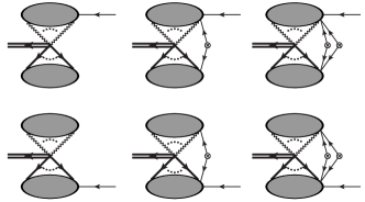
The physical consequence of Eq. (V) is the separation between the nonlinear gravitational evolution of galaxies after their creation characterized by and the more complicated nonlinear galaxy formation physics parameterized by the unknown functional . The final nonlinear growth of galaxy density perturbation relates to these two physical processes in a statistical way. Diagrammatically, Starting from the second diagram in Fig. (6), one can construct and simply by gluing initial states connected to wavy line and thick solid line separately. We illustrate in the second row of Fig. (13) up to the two-loop order.
Similarly, the second term in Eq. (V)
| (74) |
can be resummed as
| (75) |
which corresponds to the first row of Fig.(13). Therefore, up to the one-loop order, the two-point propagator of galaxy density perturbation equals
To proceed, we have to estimate the with galaxy displacement field . To the first order, the Zel’dovich approximation simply gives
| (77) |
and therefore,
| (78) |
where , and . So it is fully characterized by the gravitational growth between two different moments. Though higher order corrections analogous to the calculation in Appendix A are possible, we haven’t explicitly calculated them here. The caveat is that the galaxy displacement field at relates to at some initial Lagrangian position since we assume
| (79) |
At the lowest order , but the coordinate transform needs to be carefully incorporated for higher order calculation. Furthermore, a more reliable approach is to directly solve the fundamental dynamical equation (Eq. 14) with the potential determined by the nonlinear matter distribution at . We will leave this in the future work and simply utilize the Zel’dovich approximation (Eq. 78) within this paper.
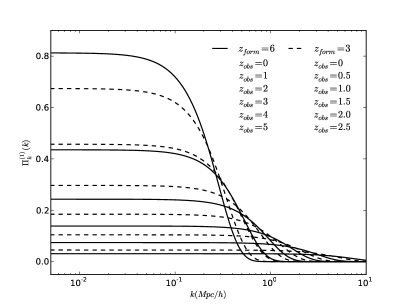
In the right panel of Fig. (14), we illustrate the from the moment of galaxy formation and evolve to various observational time . At the large scale, it converges to linear result , which relates to the linear debiasing we discussed in Eq. (48), and dampens to zero towards smaller scales with the speed proportional to . As can be seen in the figure, when galaxies have more time to evolve , i.e. is large, the observed galaxy distribution is more influenced by gravitational evolution. This can be easily seen from Eq. (V), since at tree level . When is small, vanish and therefore the gravitational evolution is negligible.
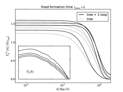
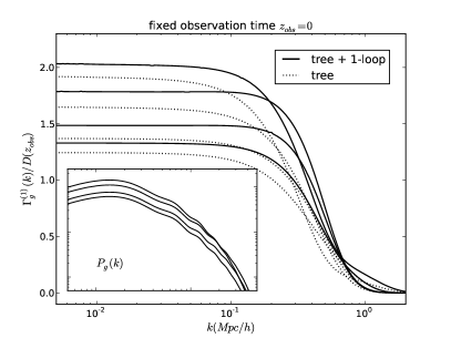
This can also be clearly seen in the left panel of Fig. (15), where we plot the normalized galaxy propagator with fixed formation redshift and observed at various . The dashed line shows the tree level of Eq. (V) and solid line corresponds to 1-loop results. In this situation, is fixed, and as decreases from to , the large scale bias also decreases as expected. However, the amplitude of the power spectrum itself as shown in the inner panel of left Fig. (15), is still increasing at lower redshift due to the linear growth . From the diagrams of three-point propagator of Eulerian bias model, at large scale , is nonzero, hence the loop integration also contributes to the large scale bias, although it’s still dominated by the tree-level value. As for smaller scales, dampens qualitatively similar to the .
In the right panel of Fig. (15), we illustrate the same quantity for fixed observation redshift , when galaxies are formed at different time with the same nonlinear process (same and ). In this case, both and are changing and the evolution of large scale bias would in principal depends on the specific parameters adopted, since the and evolve with time oppositely. In the examples we shows, dominates the evolution, i.e. galaxies formed at lower redshift would be higher biased due to the stronger nonlinear effects.
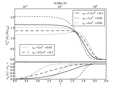
Finally, we consider the continuous galaxy formation model, assuming a simple log-normal model for average galaxy formation rate (Chan et al., 2012)
| (80) |
where is the normalization factor ensuring . Therefore, we have two parameters characterizing the model: the peak redshift of galaxy formation, and the width of the redshift for galaxy formation. In the lower panel of Fig.(16), we give several examples of galaxy formation history.
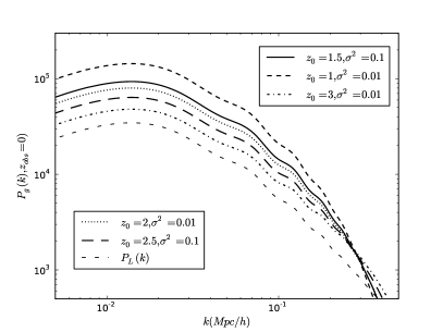
In the left-upper panel of Fig.(16), we present again the normalized propagator for various galaxy formation models which we shows in the lower panel of the same figure. As discussed previously, the here is simply a time average of weighted with . Therefore, for a narrower formation history (e.g. the dashed, dotted and dash-dotted lines), where , the results are similar to corresponding galaxy bursting models with different . On the other hand, when galaxy tends to form in a similar rate during a longer time (solid and long-dashed lines), e.g. , we are more likely to observe a galaxy power spectrum with medium amplitude and nonlinear damping. We also illustrate the corresponding power spectrum on the right panel of Fig.(16).
VI Conclusion and Discussion
An accurate modeling of the statistics of galaxy density perturbation is crucial for the success of next generation galaxy surveys. In this paper, we considered the nonlinear bias model in the context of resummed perturbation theory. In Section III, we discussed the Eulerian bias model and then generalized it to incorporate the continuous galaxy formation in Section IV. By utilizing the multipoint propagators of the matter field, our formalism for Eulerian bias model is more accurate than the standard approach in both the linear as well as the quasi-linear regimes. This has already been verified in the work of (Wang et al., 2011), where a good agreement was achieved comparing to the simulation even for the slowly converging logarithmic mapping of the density distribution. However, a detailed comparison with high-precision simulation is still needed, in at least two different levels: the accuracy of perturbative calculation itself compared to the cost of its numerical calculation, and the ability of describing the scale-dependent galaxy clustering bias at the epoch of their formation.
Furthermore, even after separating out the subsequent gravitational non-locality, the bias parameters could still be nonlocal. For example, the in Eq. (42) only counts the effective newborn galaxies that finally entered into the sample, however, such description is more or less ambiguous due to galaxy merger. Therefore, the identified progenitors in our formalism then include all merged galaxies, which would introduce a effective non-locality in the functional . In principle, this could be solved by introducing another merger contributions in the integration, but with the cost that could further complicate the model.
Acknowledgements.
XW thanks for the productive discussion with Donghui Jeong, Mark Neyrinck, Patrick McDonald and Kwan Chuen Chan. XW and AS are grateful for support from the Gordon and Betty Moore Foundations.Appendix A Matter Density Propagator in Lagrangian Perturbation Theory
Here we consider the generalized multipoint propagator
| (81) |
When , one retrieves the point propagator . For , we define as
| (82) |
As shown in Eq.(33).
| (83) | |||||
We then explicitly expands the terms inside ensemble average, which will be denoted as in the following
| (84) | |||||
Fig(4) shows all the contributions up to the one-loop order. Denotes as individual terms been summed in above equation, we have
where LPT kernel
| (86) |
Substituting the definition of into Eq.(84), one can explicit carry out up to the one-loop order,
| (87) | |||||
where we have defined a slightly different version of the integral functions introduced by Matsubara (2008a) Here we denotes
| (88) |
and
| (89) | |||||
Setting in Eq. (A), we get the up to one-loop order
which coincide with the calculation of Bernardeau (2011). For three-point
| (91) | |||||
Assuming , One recover the tree-level result ,
| (92) |
where is the second order Eulerian perturbation kernel.
Appendix B Two-loop Order of
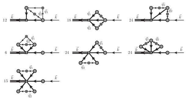
In this paper, we have calculated the two-point propagator up to two-loop order. Seven non-vanishing contributions are depicted in Fig.(17). From these diagrams, one can write down all terms explicitly
where
| (94) | |||||
Appendix C One-loop Order of
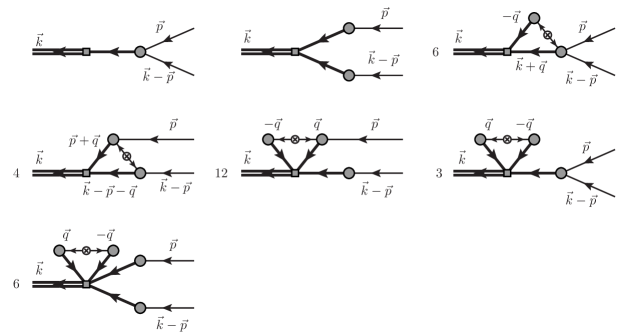
At one-loop level, five diagrams are nonzero.
where
References
- Crocce & Scoccimarro (2006a) M. Crocce and R. Scoccimarro, Phys. Rev. D 73, 063519 (2006)
- Crocce & Scoccimarro (2006b) M. Crocce and R. Scoccimarro, Phys. Rev. D 73, 063520 (2006)
- Bernardeau et al. (2008) F. Bernardeau, M. Crocce and R. Scoccimarro, Phys. Rev. D 78, 103521 (2008)
- Matsubara (2008a) T. Matsubara, Phys. Rev. D 77, 063530 (2008)
- Taruya & Hiramatsu (2008) A. Taruya and T. Hiramatsu, Astrophys. J. 674, 617 (2008)
- Pietroni (2008) M. Pietroni, JCAP 0810, 036 (2008)
- Sanchez & Cole (2008) A. G. Sanchez and S. Cole, Mon. Not. Roy. Astron. Soc. 385, 830 (2008)
- Percival et al. (2007) W. J. Percival, R. C. Nichol, D. J. Eisenstein, J. A. Frieman, M. Fukugita, J. Loveday, A. C. Pope and D. P. Schneider et al., Astrophys. J. 657, 645 (2007)
- Coles et al. (2005) S. Cole et al. [The 2dFGRS Collaboration], Mon. Not. Roy. Astron. Soc. 362, 505 (2005)
- Matsubara (2011) T. Matsubara, Phys. Rev. D 83, 083518 (2011)
- Chan et al. (2012) K. C. Chan, R. Scoccimarro and R. K. Sheth, arXiv:1201.3614 [astro-ph.CO].
- Matsubara (2008b) T. Matsubara, Phys. Rev. D 78, 083519 (2008) [Erratum-ibid. D 78, 109901 (2008)]
- Elia et al. (2011) A. Elia, S. Kulkarni, C. Porciani, M. Pietroni and S. Matarrese, Mon. Not. Roy. Astron. Soc. 416, 1703 (2011)
- McDonald (2006) P. McDonald, Phys. Rev. D 74, 103512 (2006) [Erratum-ibid. D 74, 129901 (2006)]
- McDonald (2009) P. McDonald and A. Roy, JCAP 0908, 020 (2009)
- Wang et al. (2011) X. Wang, M. Neyrinck, I. Szapudi, A. Szalay, X. Chen, J. Lesgourgues, A. Riotto and M. Sloth, Astrophys. J. 735, 32 (2011)
- Scherrer & Weinberg (1998) R. J. Scherrer and D. H. Weinberg, Astrophys. J. 504, 607 (1998)
- Tegmark & Peebles (1998) M. Tegmark and P. J. E. Peebles, Astrophys. J. 500, L79 (2011)
- Eisenstein & Hu (1998) D. J. Eisenstein and W. Hu, Astrophys. J. 496, 605 (1998)
- Bernardeau (2011) F. Bernardeau, M. Crocce and R. Scoccimarro, arXiv:1112.3895 [astro-ph.CO].