Estimating the age of renal tumors

Allen B. Downey¹¹1Professor of Computer Science, Olin College of Engineering, Needham MA 02492. Email: allen.downey@olin.edu, Web: allendowney.com

(March 2012)

Abstract

We present a Bayesian method for estimating the age of a renal tumor given its size. We use a model of tumor growth based on published data from observations of untreated tumors. We find, for example, that the median age of a 5 cm tumor is 20 years, with interquartile range 16–23 and 90% confidence interval 11–30 years.

1 Introduction

For some cancer patients it is important to estimate a tumor’s date of formation; for example, benefits provided by the U.S. Department of Veterans Affairs depend on whether it is likely that a tumor formed while the patient was in military service, among other considerations. Doctors are currently unable to provide a statistical estimate of when a tumor formed.

For renal cancers, we have reliable measurements for the rate of growth during a period of observation; this paper presents a method to use this data to estimate the distribution of ages for a renal tumor based on size at diagnosis.

1.1 Prior work

Refer to caption — Figure 1: Distribution of RDT from Zhang et al.

Several studies report growth rates for patients with untreated renal tumors [1-11]. We use this data to estimate the distribution of growth rates that is the basis of our model.

Some studies report that different subtypes grow at different rates, but Zhang et al [11] conclude “Growth rates in renal tumors of different sizes, subtypes and grades represent a wide range and overlap substantially.” Other studies are consistent with this conclusion, so our growth model does not take into account tumor subtype or grade.

2 Methodology

We use data from Zhang et al [11] to estimate the distribution of growth rates during a period of observation. We use this distribution to generate tumor growth histories. These simulations yield $P(d|t)$ , the distribution of diameter, $d$ , as a function of the age of the tumor, $t$ . Then we compute $P(t|d)$ , the distribution of age as a function of size.

2.1 Distribution of growth rates

Zhang et al report reciprocal doubling times (RDT), in units of doublings per year, for 53 “patients who underwent nephrectomy from 1989 to 2006 who did not receive preoperative chemotherapy or radiation therapy and underwent at least two preoperative contrast material-enhanced CT examinations (at least 3 months apart)”.

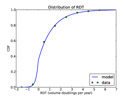
We use data from their Figure 3 to construct the cumulative distribution function (CDF) of RDT, shown in Figure 1. The line shows a model of the data as a mixture of exponential distributions: with probability $p=0.35$ we generate a negative RDT with $\lambda_{2}=5.0$ ; otherwise we generate a positive RDT with $\lambda_{1}=0.79$ . The model fits the data well, allowing us to interpolate between data points and characterize tail behavior.

2.2 Simulated growth histories

To simulate tumor growth, we start at a hypothetical time, $t_{0}$ , when tumor volume is $V_{0}=0.01$ mL (diameter 0.27 cm), and repeat these steps:

1.

Choose a random value from the modeled distribution of RDT.
2.

Compute the volume at the end of the interval, $V_{i+1}=2^{h\cdot RDT}V_{i}$ , where $h$ is the duration of the interval in years. In Zhang et al, the median time between initial and final scans is 245 days, so we used this value for the interval, $h$ .
3.

Repeat until volume exceeds $V_{max}=4200$ mL (diameter 20 cm).

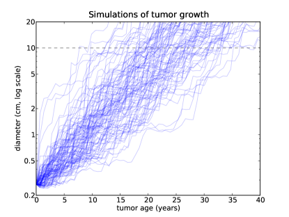
Figure 2 shows the result of 100 simulations. The vertical scale is $d$ , diameter in cm. Using these simulations, we compute $P(d|t)$ the distribution of size given $t$ , time since $t_{0}$ .

2.3 Serial correlation

Diameter	Percentiles of age
(cm)	5th	25th	50th	75th	95th
0.3	1.3	2.0	2.7	4.0	7.4
0.4	2.0	3.4	4.7	6.7	10.1
0.5	2.7	4.7	6.7	8.7	12.8
0.7	4.0	6.0	8.1	10.7	16.1
1.0	4.7	7.4	10.1	12.8	17.5
1.3	6.0	9.4	11.4	14.8	20.8
1.8	6.7	10.7	13.4	16.8	22.2
2.5	8.1	12.1	15.4	18.8	24.8
3.3	10.1	14.1	17.5	21.5	26.8
4.5	10.7	15.4	19.5	23.5	29.5
6.0	12.1	16.8	20.8	25.5	32.9
8.2	13.4	18.8	22.8	27.5	34.2
11.0	15.4	20.8	24.8	29.5	36.2
14.9	16.1	22.2	26.8	31.5	38.9

Table 1: Percentiles of time since

t_{0}

In our model of tumor growth, the growth rate during each interval is independent of previous growth rates. It is plausible that, in reality, tumors that have grown quickly in the past are more likely to grow quickly.

If this correlation exists, it affects the location and spread of our results. For example, running simulations with $\rho=0.4$ increases the estimated median age by about a year, and the interquartile range by about 3 years.

However, if there were a strong serial correlation in growth rate, there would also be a correlation between tumor volume and growth rate, and prior work has shown no such relationship [7] [11].

There could still be a weak serial correlation, but since there is currently no evidence for it, we report results based on simulations with $\rho=0$ .

2.4 Inverse probabilities

In Figure 2 the dashed line at 10 cm illustrates our method for inverting $P(d|t)$ . When a simulated history crosses this line, that represents a point in time when a tumor could be observed at this size. Since we know the duration of each history, we can construct the distribution of ages for a tumor observed at this size. Repeating this computation for each size, we construct $P(t|d)$ .

3 Results

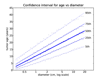
Figure 3 shows the confidence interval for $t$ as a function of size. The points are data from simulation, which produces some variability due to discrete approximation. The lines are fitted to the data. For each size, we compute the median of $t$ , interquartile range, and 90% confidence interval. Table 1 shows these results numerically, for selected sizes.

4 Conclusion

Using Table 1 we can look up the size of a tumor and find the distribution of time since $t_{0}$ , which is a lower bound on the tumor’s age. This information is potentially useful to patients, doctors and insurers.

5 References

[1] Birnbaum BA, Bosniak MA, Megibow AJ, Lubat E, Gordon RB. Observations on the growth of renal neoplasms. Radiology 1990;176:695–701.

[2] Bosniak MA. Observation of small incidentally detected renal masses. Semin Urol Oncol 1995;13:267–272.

[3] Bosniak MA, Birnbaum BA, Krinsky GA, Waisman J. Small renal parenchymal neoplasms: further observations on growth. Radiology 1995;197:589–597.

[4] Kassouf W, Aprikian AG, Laplante M, Tanguay S. Natural history of renal masses followed expectantly. J Urol 2004;171:111–113.

[5] Fujimoto N, Sugita A, Terasawa Y, Kato M. Observations on the growth rate of renal cell carcinoma. Int J Urol 1995;2:71–76.

[6] Oda T, Miyao N, Takahashi A, et al. Growth rates of primary and metastatic lesions of renal cell carcinoma. Int J Urol 2001;8:473–477.

[7] Ozono S, Miyao N, Igarashi T, et al. Tumor doubling time of renal cell carcinoma measured by CT: collaboration of Japanese Society of Renal Cancer. Jpn J Clin Oncol 2004;34:82–85.

[8] Rendon RA, Stanietzky N, Panzarella T, et al. The natural history of small renal masses. J Urol 2000;164:1143–1147.

[9] Sowery RD, Siemens DR. Growth characteristics of renal cortical tumors in patients managed by watchful waiting. Can J Urol 2004;11:2407–2410.

[10] Volpe A, Panzarella T, Rendon RA, Haider MA, Kondylis FI, Jewett MA. The natural history of incidentally detected small renal masses. Cancer 2004;100:738–745.

[11] Zhang et al., Distribution of Renal Tumor Growth Rates Determined by Using Serial Volumetric CT Measurements, January 2009 Radiology, 250, 137-144.