Theoretical Bounds on New Four-Fermion Interactions and TeV Scale Physics

Abstract:

The standard model weak interactions can be described by four-fermion $V-A$ operators at low energies. New physics at the TeV scale can, however, generate the other Lorentz structures. In this talk, we review the constraints on such interactions from nuclear and hadronic decays, as well as from collider searches. Currently the most stringent bounds come from the analysis of the $0^{+}\to 0^{+}$ nuclear and the $\pi\to e\nu\gamma$ radiative pion decays. In the near future, the ultracold neutron beta decay experiments and the direct LHC measurements will compete in setting the most stringent bounds, provided, however, that the neutron-to-proton non-perturbative transition matrix elements can be calculated to a level of 10–20% accuracy.

1 Effective Lagrangian for the Charge-Current Interactions

We follow the notation of Ref. [1], which identified a minimal basis for the $SU(2)_{L}\times U(1)_{Y}$-invariant dimension-six operators contributing to low-energy charged-current processes. In particular, we study only theories that do not violate $CP$ and conserve baryon and lepton numbers at this level, and that do not contain light right-handed neutrinos. In such theories, we can write the part of this charged-current Lagrangian coupling quarks to leptons as

$${\cal L}_{\rm CC} = \frac{-g^{2}}{2M_{W}^{2}}V_{ij}\Bigg{[}\Big{(}1+[v_{L}]_{\ell\ell^{\prime}ij}\Big{)}\bar{\ell}_{L}\gamma_{\mu}\nu_{\ell^{\prime}L}\bar{u}_{L}^{i}\gamma^{\mu}d_{L}^{j}+[v_{R}]_{\ell\ell^{\prime}ij}\bar{\ell}_{L}\gamma_{\mu}\nu_{\ell^{\prime}L}\bar{u}_{R}^{i}\gamma^{\mu}d_{R}^{j}$$ (1)

$$+ [s_{L}]_{\ell\ell^{\prime}ij}\bar{\ell}_{R}\nu_{\ell^{\prime}L}\bar{u}_{R}^{i}d_{L}^{j}+[s_{R}]_{\ell\ell^{\prime}ij}\bar{\ell}_{R}\nu_{\ell^{\prime}L}\bar{u}_{L}^{i}d_{R}^{j}$$

$$+ [t_{L}]_{\ell\ell^{\prime}ij}\bar{\ell}_{R}\sigma_{\mu\nu}\nu_{\ell^{\prime}L}\bar{u}_{R}^{i}\sigma^{\mu\nu}d_{L}^{j}\Bigg{]}+{\rm h.c.}\,,$$

where we have suppressed the color indices and used the notation $\sigma^{\mu\nu}=i[\gamma^{\mu},\gamma^{\nu}]/2$. Further, $g$ is the weak coupling, $M_{W}$ is the mass of the $W$-boson, $V_{ij}$ refer to the CKM matrix elements, $L$ and $R$ to the chiral projections, $\ell$ and $\ell^{\prime}$ to the lepton families, $i$ and $j$ to the quark families, $u$ and $d$ to the generic up and down type quarks, and $\ell$ and $\nu_{\ell}$ to the charged leptons and neutrinos, respectively. This effective theory contains five families of effective couplings: $v_{L}$, $v_{R}$, $s_{L}$, $s_{R}$, and $t_{L}$, which are expected to be of order $v^{2}/\Lambda^{2}\sim 10^{-3}$, where $v$ is the Higgs VEV and $\Lambda$ is the scale of new physics. Even though we write only the charged current sector here, we note that due to the $SU(2)$ invariance of the interactions, the same effective couplings also mediate neutral current interactions that can be used to constrain them.

For the most part we will be interested only in the first family of the quarks and work to linear order in the effective BSM couplings. Also suppressing the lepton family indices, we can write

$${\cal L}_{\rm CC} = -\frac{G_{F}^{(0)}V_{ud}}{\sqrt{2}}\Big{(}1+\epsilon_{V}\Big{)}\Bigg{[}\bar{\ell}\gamma_{\mu}(1-\gamma_{5})\nu\cdot\bar{u}\Big{[}\gamma^{\mu}(1-\gamma_{5})+\big{(}\epsilon_{V}-\epsilon_{A}\big{)}\gamma^{\mu}\gamma_{5}\Big{]}d$$ (2)

$$+ \bar{\ell}(1-\gamma_{5})\nu_{\ell}\cdot\bar{u}\Big{[}\epsilon_{S}-\epsilon_{P}\gamma_{5}\Big{]}d+\epsilon_{T}\bar{\ell}\sigma_{\mu\nu}(1-\gamma_{5})\nu\cdot\bar{u}\sigma^{\mu\nu}(1-\gamma_{5})d\Bigg{]}+{\rm h.c.}\,,$$

where $G^{(0)}_{F}$ is the tree-level Fermi constant, $\epsilon_{V,A}\equiv v_{L}\pm v_{R}$, $\epsilon_{S,P}\equiv s_{L}\pm s_{R}$, $\epsilon_{T}\equiv t_{L}$. In this notation, $\epsilon_{V}$ affects the overall normalization of the Fermi constant and is constrained both from low-energy and Z-pole observables. The right handed vector coupling, $\epsilon_{V}-\epsilon_{A}$, however, only affects the ratio of Axial-to-Vector couplings and constraining it meaningfully from hadronic physics needs determination of the rato of vector and axial charges to better than $10^{-3}$ level. The rest of the couplings $\epsilon_{S,P,T}$ violate chirality and, hence, their intereference with the Standard Model interactions is suppressed by $m_{\ell}/E$; consequently, they are suppressed in high-energy experiments, but remain accessible in pion decays and asymmetry measurements in beta decays.

2 Collider Limits

The BSM couplings can be directly probed at colliders as excess large transverse mass events in the channel $pp\to e\bar{\nu}+X$. Using the CMS report that the excess in this channel at $m_{T}>1\ {\rm TeV}$ is less than 3.7 events in $1.13\ {\rm fb}^{-1}$ of data at $\sqrt{s}=7\ {\rm TeV}$ [2], we can, therefore, obtain bounds on the BSM couplings. As discussed later, and shown in Fig. 2, these bounds are currently weaker than the bounds obtained from low energy experiments.

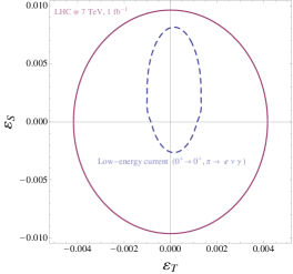
Figure 1: The bounds on the BSM scalar and tensor interactions obtained at LHC compared to those from low-energy measurements.

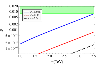
Figure 2: Lower bounds on $\epsilon_{S}$ at 2 GeV given collider discovery cross-sections of 100, 10, and 2 fb at a center-of-mass energy of $\sqrt{s}=14\ {\rm TeV}$.

The collider bounds, however, get considerably stronger if the scalar interaction is due to a resonance that is accessible at the LHC energies. If this new resonance couples to the quarks with a coupling constant $g_{q}$ and to the leptons with $g_{l}$, then the partial cross section can be written as

$$\sigma=g_{q}^{2}g_{l}^{2}\frac{m_{S}}{48s\,\Gamma_{S}}L(\tau)\,,$$ (3)

where $s$ is the square of the center-of-mass energy, $\tau\equiv m^{2}/s$, $L(\tau)$ is the relevant parton-distribution function and $m_{S}$ and $\Gamma_{S}$ are the mass and width of the resonance. With these couplings, the resonance can decay at least to quarks and leptons, so we have

$$\Gamma_{S}\geq(g_{l}^{2}+2N_{c}g_{q}^{2})\frac{m}{16\pi}\,,$$ (4)

where $N_{c}$ is the number of colors in the theory. At low energies, the same couplings give a contribution to $\epsilon_{S}$:

$$\epsilon_{S}=2g_{q}g_{l}\frac{v^{2}}{m^{2}}\geq\frac{12v^{2}\sqrt{2N_{c}}}{\pi\tau L(\tau)}\sigma\,.$$ (5)

As shown in Fig. 2, this implies that for reasonable discovery cross-sections of 100 fb at $\sqrt{s}=14\ {\rm TeV}$, a low-energy measurement sensitivity of $10^{-4}$ on $\epsilon_{S}$ is highly competitive.

3 Neutron beta decay

All of the BSM four-fermion operators contribute to the neutron beta decay $n(p_{n})\to\allowbreak p(p_{p})\allowbreak e^{-}(p_{e})\allowbreak\bar{\nu}_{e}(p_{\nu})$. The transition matrix elements of the quark bilinears required to analyze this can be parameterized as [3]

$$\mathopen{\left\langle p(p_{p})\right|}\bar{u}\gamma_{\mu}d\mathclose{\left|n(p_{n})\right\rangle} = \bar{u}_{p}(p_{p})\left[g_{V}(q^{2})\gamma_{\mu}+\frac{\tilde{g}_{T(V)}(q^{2})}{2M_{N}}\sigma_{\mu\nu}q^{\nu}+\frac{\tilde{g}_{S}(q^{2})}{2M_{N}}q_{\mu}\right]u_{n}(p_{n})\,,$$

$$\mathopen{\left\langle p(p_{p})\right|}\bar{u}\gamma_{\mu}\gamma_{5}d\mathclose{\left|n(p_{n})\right\rangle} = \bar{u}_{p}(p_{p})\left[g_{A}(q^{2})\gamma_{\mu}+\frac{\tilde{g}_{T(A)}(q^{2})}{2M_{N}}\sigma_{\mu\nu}q^{\nu}+\frac{\tilde{g}_{P}(q^{2})}{2M_{N}}q_{\mu}\right]\gamma_{5}u_{n}(p_{n})\,,$$

$$\mathopen{\left\langle p(p_{p})\right|}\bar{u}d\mathclose{\left|n(p_{n})\right\rangle} = g_{S}(q^{2})\bar{u}_{p}(p_{p})u_{n}(p_{n})\,,$$ (6c)

$$\mathopen{\left\langle p(p_{p})\right|}\bar{u}\gamma_{5}d\mathclose{\left|n(p_{n})\right\rangle} = g_{P}(q^{2})\bar{u}_{p}(p_{p})\gamma_{5}u_{n}(p_{n})\,,$$ (6d)

$$\mathopen{\left\langle p(p_{p})\right|}\bar{u}\sigma_{\mu\nu}d\mathclose{\left|n(p_{n})\right\rangle} = \bar{u}_{p}(p_{p})\left[g_{T}(q^{2})\sigma_{\mu\nu}+g_{T}^{(1)}(q^{2})\left(q_{\mu}\gamma_{\nu}-q_{\nu}\gamma_{\mu}\right)\right.$$ (6e)

$$+ \left.g_{T}^{(2)}(q^{2})\left(q_{\mu}P_{\nu}-q_{\nu}P_{\mu}\right)+g_{T}^{(3)}(q^{2})\left(\gamma_{\mu}\not{q}\gamma_{\nu}-\gamma_{\nu}\not{q}\gamma_{\mu}\right)\right]u_{n}(p_{n})\,,$$

where $u_{p,n}$ are the proton and neutron spinor amplitudes, $P=p_{n}+p_{p}$, $q=p_{n}-p_{p}$ is the momentum transfer, and $M_{N}=(M_{n}+M_{p})/2$ denotes an isospin-invariant nucleon mass.

Note that we are interested in disentangling the effects of $\epsilon_{P,S,T}$ which are expected to be about $10^{-3}$ when induced by BSM physics at the TeV scale. This is the same size as the recoil corrections of order $q/M_{N}$, as well as the radiative corrections proportional to $\alpha_{s}/\pi$ and isospin breaking effects proportional to $(M_{n}-M_{p})/M_{N}$. In the above equation, all the spinor contractions are $O(1)$, except for $\bar{u}_{p}\gamma_{5}u_{n}$ which is $O(q/M_{N})$. Furthermore, only the vector and axial vector bilinears appear in the standard model, the rest are pure BSM corrections and appear multiplied by $\epsilon_{S,P,T}$. Finally, the change in the form factors between zero momentum and the finite recoil are proportional to $q^{2}/\Lambda_{\rm QCD}^{2}\sim 10^{-5}$. In light of this, we now discuss the contributions from these bilinears that are relevant to the linear order in a simultaneous expansion in $\epsilon$, $q/M_{N}$, $(M_{n}-M_{p})/M_{N}$, $q^{2}/\Lambda_{\rm QCD}^{2}$ and $\alpha_{s}/\pi$.

• Vector Current: The form factor $g_{V}(0)$ contributes to the leading order, whereas the weak magnetic charge $\tilde{g}_{T(V)}(0)$ contributes to the first order in $q/M_{N}$. The former is $1$ up to second-order corrections in isospin breaking and the latter can be related to the difference of proton and neutron magnetic moments by isospin symmetry. Both of these are, therefore, known to the required accuracy. The induced-scalar form factor, $\tilde{g}_{S}(0)$, vanishes in the isospin limit and is further proportional to $q_{\mu}/M_{N}$, so it can be neglected to this order.

• Axial Current: $g_{A}(0)$ contributes to this marix element at our required order. The induced-tensor form factor, $\tilde{g}_{T(A)}(0)$, vanishes in the isospin limit and has an explicit $q_{\mu}/M_{N}$, whereas the induced pseudoscalar, $\tilde{g}_{P}(0)$, is proportional both to $q_{\mu}/m_{N}$ and to the pseudoscalar spinor contraction that it is also of order $q_{\mu}/m_{N}$.

• Pseudoscalar bilinear: This entire term is subleading since the pseudoscalar contraction is proportional to $q_{\mu}/m_{N}$ and the contribution is also proportional to a BSM coupling.

• Scalar and Tensor bilinears: The terms proportional to $g_{S}(0)$ and $g_{T}(0)$ are $O(1)$ and multiplied by the BSM couplings $\epsilon_{S}$ and $\epsilon_{T}$. The $g_{T}^{(1,2,3)}$ contributions are subleading since they are multiplied by an explicit factor of $q^{\mu}/m_{N}$.

In summary, the only matrix elements that feed into the leading order determination of the BSM coefficients, and are not directly constrained by experiments to the required order, are $g_{A}(0)$, $g_{S}(0)$, and $g_{T}(0)$. Furthermore, the BSM coefficient $\epsilon_{V}$ can be absorbed into a redefined Fermi constant $\tilde{G}_{F}^{(0)}\equiv G_{F}^{(0)}(1+2\epsilon_{V})$, and $\epsilon_{A}$ can similarly be used to redefine the ratio of axial and vector charges: $\tilde{\lambda}\equiv(\epsilon_{V}-\epsilon_{A})g_{A}(0)/g_{V}(0)$.

The differential decay distribution of the neutron is given by [4, 5]

$$\frac{d\Gamma}{dE_{e}d\Omega_{e}d\Omega_{\nu}} = \frac{(\tilde{G}_{F}^{(0)})^{2}\,|V_{ud}|^{2}}{(2\pi)^{5}}\left(1+3\,\tilde{\lambda}^{2}\right)\cdot w(E_{e})\cdot D(E_{e},\mathbf{p}_{e},\mathbf{p}_{\nu},\boldsymbol{\sigma}_{n})\,,$$ (7)

where $\mathbf{p}_{e}$ and $\mathbf{p}_{\nu}$ denote the electron and neutrino three-momenta, and $\boldsymbol{\sigma}_{n}$ denotes the neutron polarization. The bulk of the electron spectrum is described by

$$w(E_{e})=p_{e}E_{e}(E_{0}-E_{e})^{2}\times{\rm rad.corr.}\,,$$

where $E_{0}=\Delta-(\Delta^{2}-m_{e}^{2})/(2M_{n})$ (with $\Delta=M_{n}-M_{p}$) is the electron endpoint energy, $m_{e}$ is the electron mass, and $\rm rad.corr.$ stands for the Coulomb and radiative corrections [4, 5, 6]. The remaining differential decay distribution function $D(E_{e},\mathbf{p}_{e},\mathbf{p}_{\nu},\boldsymbol{\sigma}_{n})$ is parameterized as [4, 5, 7]

$$D(E_{e},\mathbf{p}_{e},\mathbf{p}_{\nu},\boldsymbol{\sigma}_{n})=1+c_{0}+c_{1}\frac{E_{e}}{M_{N}}+\frac{m_{e}}{E_{e}}\bar{b}+\bar{B}(E_{e})\frac{\boldsymbol{\sigma}_{n}\cdot\mathbf{p}_{\nu}}{E_{\nu}}+\bar{A}(E_{e})\frac{\boldsymbol{\sigma}_{n}\cdot\mathbf{p}_{e}}{E_{e}}+\ldots\,,$$ (8)

where $c_{0,1}$ are recoil corrections, $\bar{b}$ is a Fierz interference term, $\bar{A}(E_{e})$ and $\bar{B}(E_{e})$ describe the angular correlations between outgoing momenta and the neutron spin, and the correlations between the outgoing electron and neutrino momenta are not shown. An important point to note is that experiments usually measure the angular dependence by measuring the decay asymmetry, i.e. the decay rate in some ‘forward’ and ‘backward’ bins normalized by the total decay rate. Since the Fierz intereference term appears in this normalization, extraction of BSM contributions to these asymetries is always contaminated by the BSM contributions to $b$.

The BSM scalar and tensor interactions appear to linear order in the above decay matrix element in only two terms [9]:

$${\bar{b}}^{\rm BSM} \approx 0.34g_{S}\epsilon_{S}-5.22g_{T}\epsilon_{T}\,,$$ (9a)

$${\bar{b}}_{\nu}\equiv\left.E_{e}\frac{\partial\bar{B}^{\rm BSM}(E_{e})}{\partial m_{e}}\right|_{m_{e}=0} \approx 0.44g_{S}\epsilon_{S}-4.85g_{T}\epsilon_{T}\,,$$ (9b)

where all the matrix elements are evaluated at zero momentum transfer. Currently both of these quantities have extremely weak bounds: they are known to lie in the interval $[-0.3,0.5]$ at 95% Confidence Level. Experiments to measure these quantities to the level of $10^{-3}$ are under way [10]. Additionally, the scalar and tensor charges of the nucleon are very poorly constrained by phenomenology [11]: $0.25<g_{S}<1.0$ and $0.6<g_{T}<2.3$, and current lattice estimates also have large uncertainties: $g_{S}=0.8(4)$ and $g_{T}=1.05(35)$ [9]. In Fig. 3, we show the impact of a $10^{-3}$ level measurement with these uncertainties on the estimates of the charges, though lattice calculations are under way to improves these estimates [12].

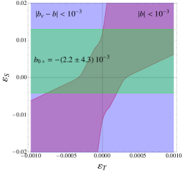
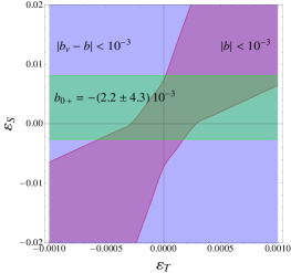
Figure 3: 90% Confidence Intervals of allowed regions in the $\epsilon_{S}$-$\epsilon_{T}$ plane by the existing bounds on $0^{+}\to 0^{+}$ nuclear beta decay life times and the projected measurements of the neutron decay asymmetry at the $10^{-3}$ level. The left panel shows the results with the scalar and tensor charges constrained by phenomenology, whereas the right panel uses the current lattice estimates.

4 Low Energy Phenomenology

The BSM coefficients $\epsilon_{S,P,T}$ are also constrained by various nuclear beta decays. In particular, the half lives of various $0^{+}\to 0^{+}$ decays constrain the scalar coupling [13] to a 90% Confidence Interval (CI) of $-1\times 10^{-3}<g_{S}\epsilon_{S}<3.2\times 10^{-3}$. The tensor coupling, on the other hand, can be constrained by studying pure Gamow-Teller transitions; the 90% CI from ⁶⁰Co and ¹¹⁴In are $-2.9\times 10^{-3}<g_{T}\epsilon_{T}<1.5\times 10^{-2}$ [14] and $-2.2\times 10^{-3}<g_{T}\epsilon_{T}<1.3\times 10^{-2}$ [15], respectively. Further bounds can be obtained by studying the angular and momentum correlations in various beta decays, and some of the best 90% CIs from such measurement are $-0.76\times 10^{-2}<g_{S}\epsilon_{S}+0.18g_{T}\epsilon_{T}<1.0\times 10^{-2}$ and $|g_{T}\epsilon_{T}|<3.1\times 10^{-3}$ from positron polarization measurements [16, 17, 18], and $|g_{T}\epsilon_{T}|<6\times 10^{-3}$ from beta-neutrino momentum correlations [19].

The pion decays are very precisely measured and can also be used to constrain the BSM couplings. In particular, the branching ratio of pion decays to electrons,

$$R_{\pi}\equiv\frac{\Gamma(\pi\to e\nu[\gamma])}{\Gamma(\pi\to\mu\nu[\gamma])}\,,$$ (10)

is very well constrained. This BSM contribution is given as

$$\frac{R_{\pi}}{R_{\pi}^{SM}}=\frac{\left(1-\frac{B}{m_{e}}\epsilon_{P}^{ee}\right)^{2}+\left(\frac{B}{m_{e}}\epsilon_{P}^{e\mu}\right)^{2}+\left(\frac{B}{m_{e}}\epsilon_{P}^{e\tau}\right)^{2}}{\left(1-\frac{B}{m_{\mu}}\epsilon_{P}^{\mu\mu}\right)^{2}+\left(\frac{B}{m_{\mu}}\epsilon_{P}^{\mu e}\right)^{2}+\left(\frac{B}{m_{\mu}}\epsilon_{P}^{\mu\tau}\right)^{2}}\,.$$ (11)

Unless there are accidental cancellations, the quadratic terms in the denominator can be neglected. The contribution of the quadratic terms in the numerator is, however, enhanced by the large coefficient $B/m_{e}\approx 3.6\times 10^{3}$ in $\overline{\rm MS}$ at 1 GeV. The experimental constraint $R_{\pi}/R_{\pi}^{SM}=0.996\pm 0.005$ at 90% confidence then allows only a small spherical shell in $\epsilon_{P}^{ee,\mu,\tau}$ space that is centered at $2.75\times 10^{-4},0,0$ with a radius of $2.75\times 10^{-4}$ and a thickness of $1.38\times 10^{-6}$. Therefore, without assuming any relation between the various pseudoscalar couplings, one can only bound them as

$$-1.4\times 10^{-7}{}<\epsilon_{P}^{ee}<{}5.5\times 10^{-4}\,,\qquad-2.75\times 10^{-4}{}<\epsilon_{P}^{e\mu,\tau}<{}2.75\times 10^{-4}\,.$$ (12a)

Standard model radiative corrections, however, mix the scalar, tensor, and pseudoscalar couplings:

$$\epsilon_{P}(\mu) = \epsilon_{P}(\Lambda)\left(1+1.3\times 10^{-2}\log\frac{\Lambda}{\mu}\right)$$ (13)

$$\quad+6.7\times 10^{-4}\epsilon_{S}(\Lambda)\log\frac{\Lambda}{\mu}-7.3\times 10^{-2}\epsilon_{T}(\Lambda)\log\frac{\Lambda}{\mu}\,,$$

where we have suppressed the family indices. As a result, barring cancellations, the stringent constraints on the pseudoscalar coupling translate to constraints on scalar and tensor couplings as well: $|\epsilon_{S}|\lesssim 8\times 10^{-2}$ and $|\epsilon_{T}|\lesssim 10^{-3}$. The constriaint on the tensor is similar to that obtained directly from the radiative branching fraction of the pion decay: $-2\times 10^{-4}<\epsilon_{T}f_{T}<2.6\times 10^{-4}$, where $f_{T}$, the tensor charge of the pion, is estimated to be $0.24\pm 0.04$.