State Space Exploration of RT Systems in the Cloud

Abstract

The growing availability of distributed and cloud computing frameworks make it possible to face complex computational problems in a more effective and convenient way. A notable example is state-space exploration of discrete-event systems specified in a formal way.

The exponential complexity of this task is a major limitation to the usage of consolidated analysis techniques and tools. We present and compare two different approaches to state-space explosion, relying on distributed and cloud frameworks, respectively. These approaches were designed and implemented following the same computational schema, a sort of map & fold. They are applied on symbolic state-space exploration of real-time systems specified by (a timed extension of) Petri Nets, by readapting a sequential algorithm implemented as a command-line Java tool. The outcome of several tests performed on a benchmarking specification are presented, thus showing the convenience of cloud approaches.

I Introduction

State-space exploration is the most widely used technique for the analysis of discrete-event systems specified in a formal way, due to the completeness of provided information, and the possibility of being easily automated. However, a known major weakness of this approach is the possible combinatorial growing of state-space with respect to models’ size [13].

A typical application area of state-space exploration is the validation of Real-Time (RT) systems, that require intensive verification before deployment. Several formal models for RT systems have been proposed [8], among which time extensions of Petri nets (PN) play an important role. The verification of RT properties, that mix logical and timing aspects, usually requires building directed graphs expressing the system behavior in terms of state-transitions [3, 8], starting from an initial state. RT constraints make this an even more challenging task. In the case of a dense time domain, the set of reachable states is likely to be infinite: this is normally tackled by clustering classes of states which share some reachability and timing conditions [3, 8]. Yet, time breaks the locality of events’ occurrences that is a key feature in classical state-space exploration techniques.

We introduce and compare two different approaches to state-space exploration, based on distributed and cloud computing frameworks. Although these approaches do not alleviate state-space explosion, they lead to a significant speed-up of execution times (by considerably increasing the storage space and computation power at disposal) and permit computing resources to be scaled up.

In accordance to a consolidated idea, independent processing units (sw or hw) are in charge of building partitions of the state-transition graph, synchronizing at the end of the computation in order to consistently compose the whole structure. What characterizes our approaches, making them parametric to the adopted formalisms, is a full adherence to a computational pattern which lies in iterating a sequence of elementary “map-fold” operations. For example they could be easily specialized to work with different kinds of PNs, or they could be exploited in the context of model-checking for efficiently translating Labeled Transition System (LTs) from an implicit representation to an explicit one [9].

Our reference model is Time-Basic (TB) nets [11], an expressive formalism for RT systems’ specification. An efficient state-space exploration technique for TB nets was recently implemented as a sequential Java program [3]. The output is a symbolic state-transitions graph (TRG), that overcomes the old analyzer of TB nets [4] (based in turn on a time-bounded inspection of a symbolic tree). In this paper we present how we have adapted the sequential TRG builder in order to exploit distributed/cloud computing frameworks. A summary of test sessions carried out on a benchmarking system specification (the Gas Burner [2, 4]) is also included. The proposed approaches are shown to significantly improve the sequential algorithm performances, both in terms of execution time and analyzable model’s size.

I-A TB nets and timed reachability analysis

TB nets [11] belong to the category of formalisms in which time constraints on systems’ state transitions are expressed as numerical intervals, denoting the possible instants at which some events may occur. Intervals’ domain is assumed here $\mathbb{R}^{+}$. TB nets are very expressive, for two main reasons: first, interval bounds are functions of the time description of a state; secondly, each event occurrence may be assigned either a weak or a strong semantics: under some conditions, a given event either may or must occur.

Let us recall a few computationally relevant points of the TRG algorithm proposed in [3]. We here omit unessential details related to the employed formalism.

A TRG node represents a symbolic state $S=\langle M,C\rangle$, where $M$ is the topological description of a system state given in terms of symbols denoting time-stamps (a marking, following the PNs parlance), $C$ is a predicate expressed as linear inequalities involving such symbols. Assuming no absolute time references are used in a TB model, $C$ only contains relative time dependencies, e.g., $T_{2}-T_{1}\leq 1.5\wedge T_{0}\leq T_{1}$. The most expensive task is verifying inclusion between nodes, meant as classes of corresponding ordinary states: when a successor $S^{\prime}$ of node $S$ is generated, we check whether any node $S^{\prime\prime}$ already exists such that either $S^{\prime}\subseteq S^{\prime\prime}$ or $S^{\prime}\supset S^{\prime\prime}$ (in the latter case $S^{\prime}$ absorbs $S^{\prime\prime}$, and it is set “to be processed”). A symbolic state normalization is required, involving different actions. First, symbols occurring in $C$, but not in $M$, are eliminated. What constitutes the key point of the whole algorithm — and very often enables termination — however, is a quite sophisticated procedure able to recognize symbols that are irrelevant for the model evolution. Such symbols are replaced in $M$ by anonymous time-stamps, then they are possibly eliminated from $C$. Let $S$, $S^{\prime}$ be normalized: a sufficient condition for $S\subseteq S^{\prime}$ is $M=M^{\prime}$ and $C\wedge\neg C^{\prime}\equiv false$ .

II Sequential model

The TRG construction has been automated by means of a Java tool called $Graphgen$. The corresponding sequential algorithm is sketched in the Fig. 1.

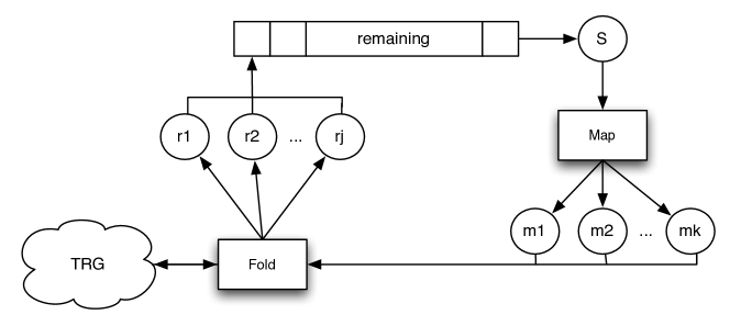
Figure 1: Sequential model

The remaining list contains the reachable nodes of the graph not yet examined, i.e., the expansion front of the graph. The graph builder takes one node at a time from the expansion front and executes two main phases: Map and Fold. These operations derive from a well known programming model in which a Map instance takes as input a sequence of values and computes a given function for each value. Then, a Fold instance combines in some way the elements of the sequence using an associative binary operation.

In the TRG builder, the Map generates the successors of a node, the Fold combines them with the already existing nodes by identifying possible inclusion relationships. Whenever the Fold phase identifies a relation between a new node $A$ (just computed by the Map) and an old node $B$ (already expanded), different operations must be performed on the adjacent edges depending on the relation between $A$ and $B$.

• If $A\subseteq B$, the incoming edges of $A$ are redirected to $B$. The outgoing edges are not yet calculated, thus no actions are required.

• If $A\supset B$, the incoming edges of $B$ are redirected to $A$ and the outgoing edges of $B$ (subset of the A’s ones) are removed.

At the end of the Fold phase the nodes computed by the Map which are not included in any old nodes, are placed into the remaining list. The Map phase and the Fold phase are repeated until the expansion front becomes empty.

III Parallel models

The sequential TRG builder execution takes more than 7 hours even for a relatively small example as the Gas Burner is. It is however possible to identify independent computational sequences, in order to exploit the TRG algorithm in multi-thread and distributed frameworks. We conceived two different ways for organizing parallel computations. The two models are described in the following.

Workers model

This model parallelizes the processing of nodes in the expansion front. A set of independent computational units (Workers, see Fig. 2) locally execute the Map and Fold phases. Each Worker computes a portion of the final graph by examining a set of similar nodes. The whole state space is partitioned among the Workers by applying to each reachable state $S$ the following function:

$$\operatorname{\mathrm{Hash}}(f(S))\bmod n$$ (1)

where $n$ is the number of Workers, and $f$ extracts some features from $S$ ensuring that the equality of $f(S)$ is a necessary condition for inclusion relationships. In our implementations, $f$ is an easy to compute abstraction on $M$ — called soft marking — such that the equality of soft markings is a necessary condition for two symbolic states to be included into one another. The first definition of soft marking we used disregards the identity of time-stamp symbols. Let $|M(p)|$ be the number of tokens in the place $p$. The soft marking of a state $S$ is defined as:

$$\begin{split}f(S)=\langle|M(p_{1})|,...,|M(p_{k})|\rangle\,\in\mathbb{N}^{k}\end{split}$$ (2)

where $p_{1},...,p_{k}$ are the places of the analyzed TB net.

Thus, any two nodes possibly related by inclusion are assigned to the same Worker. Therefore, each Worker is able to locally accomplish the fold operation. Then it sends the mapped nodes for which it is not responsible to the appropriate peers. Fig. 2 shows the overall architecture of this model: each Worker has its own remaining list, which contains nodes not yet examined. The expansion front is now the overall union of all local remaining lists.

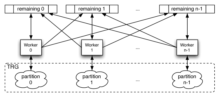
Figure 2: Workers model

Mappers & Folders model

The second model specializes the Workers in Mappers and Folders (see Fig. 3). A Mapper computational unit takes nodes from the expansion front, it maps them into their successors, and assigns the map outcome to the proper Folders by means of the Hash function (1) where $n$ is the number of Folders; they in turn identify possible inclusion relationships, and build partitions of the whole final graph.

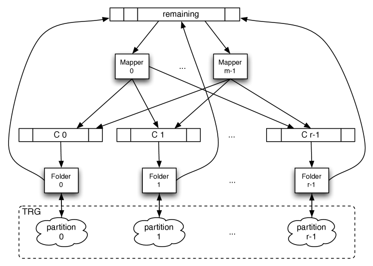
Figure 3: Mappers & Folders model

It is worth noting that with respect to ordinary state-space exploration techniques, both parallel models incur in additional overheads due to extra communication and synchronization, greatly affecting speed-up. The main overheads are due to the frequent locking of the structure recording symbolic nodes (usually represented as hash tables), and to the load imbalance deriving from asymmetric computations performed by Workers.

Therefore, the conceptually global symbolic structure (the TRG) is partitioned among different computational units, according to the rule that each unit stores a set of nodes associated with the incoming edges. This choice makes the distributed management of the TRG easier: the only synchronization point is raised by the erasure (due to absorption) of nodes with outgoing edges. These information is not locally present because outgoing edges are stored in the target nodes, which are potentially belonging to other units. To minimize further the communications between computational units, we perform a delayed removal of pending edges (outgoing edges of removed nodes) at the end of the global computation. For instance, the node $a$ represented in Fig. 4 is included in $b$. The redirection of the incoming edges ($f\rightarrow a$ and $c\rightarrow a$) can be performed locally because $a$ and $b$ belong to the same partition. The removal of outgoing edges ($a\rightarrow e$ and $a\rightarrow d$), instead, cannot be performed locally because $e$ and $d$ are not present in the partition $i$.

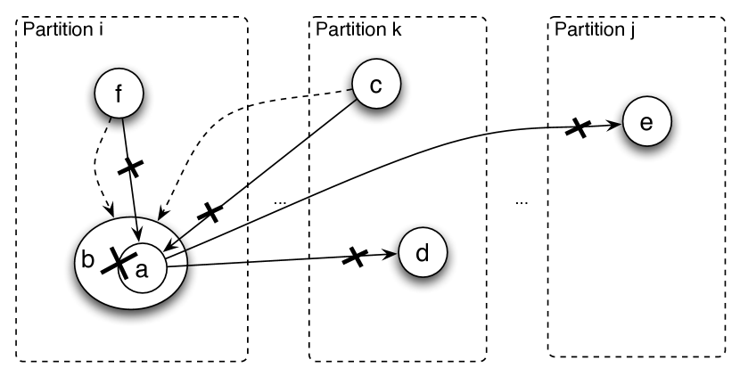
Figure 4: Operations on edges during the Fold phase.

IV Distributed implementations

In order to scale to a large number of computational units we considered different distributed architectures. In particular we used two existing frameworks: JavaSpaces [7] and Hadoop MapReduce [12]. In this way we concentrated on the functional aspects of our distributed application, while leaving to the frameworks the management of fault tolerance and low-level communication. While the JavaSpaces implementation has been designed to run on local networks, MapReduce has the possibility to be deployed “in the cloud” in order to easily exploit a larger number of machines with better installed hardware.

IV-A JavaSpaces Tool

JavaSpaces technology is a high-level tool for building distributed applications, and it can also be used as a coordination tool. It has its roots in the Linda coordination language [10]. Departing from more traditional distributed models that rely on message passing or RMI, the JavaSpaces model views a distributed application as a collection of processes that use a persistent storage (one or more spaces) to store objects and to communicate.

By using this framework we have implemented the first parallel model presented in Section III (Fig. 2). We implemented each remaining list as a space where Worker processes can exchange states not yet examined. There is also one coordinator process that initializes the computation by producing the initial state, then waits for the termination of each Worker in order to merge the computed partitions into the final TRG. The overall architecture is presented in Fig. 5.

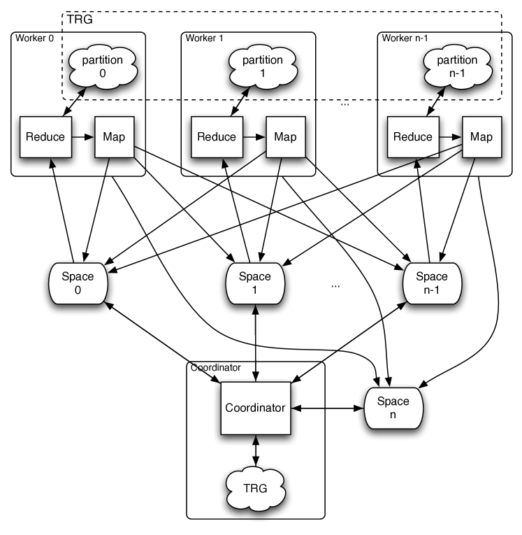
Figure 5: Distributed JavaSpaces model

IV-B Hybrid Iterative MapReduce

This is a distributed implementation of the second parallel model presented in Section III (Fig. 3). MapReduce is a well known programming model with associated implementations, for writing applications that rapidly process vast amounts of data in parallel on large clusters of computational cores. Users specify a Map function that processes a key/value pair to generate a set of intermediate key/value pairs, and a Reduce function that merges intermediate values associated to the same intermediate key.

$$\begin{split}\texttt{Map}(k_{1},v_{1})\rightarrow list(k_{2},v_{2})\\ \texttt{Reduce}(k_{2},list(v_{2}))\rightarrow list(v_{2})\end{split}$$ (3)

In order to exploit this programming model we represent our data set as pairs $\langle f(S),S\rangle$ , where $S$ is a node of the symbolic $TRG$ with associated incoming edges, $f(S)$ is the soft marking defined in (1).

We actually used an extended version of the original MapReduce model introduced in [5]. With respect to such a model, MapReduce jobs are iterated until the expansion front becomes empty. This is called “Iterative MapReduce” [6]. Each iteration maps all nodes in the expansion front, then it reduces the new nodes by identifying possible inclusion relationships. Note that the reduce phase requires all the $TRG$ nodes in order to identify each potential inclusion relationship between them. For this reason, the input of each iteration is made up by a set of $new$ nodes (the expansion front) and a set of $old$ nodes (the $TRG$ portion till now computed).

A Map takes a pair $\langle f(S),S\rangle$ as input. If it corresponds to an old node it is just passed to the reduce phase, without being processed. Otherwise, the set $\{\langle f(S^{\prime}),S^{\prime}\rangle\}$ of the states directly reachable from $S$ is computed, and it is passed to the reduce phase together with $\langle f(S),S\rangle$ itself. After the map phase is concluded, an intermediate shuffle phase brings together pairs with the same soft marking ($f(S)$) and it gives each group to a different Reduce. A Reduce erases the values (states) that are shown to be included in some other and it gives in output a set of values forming a partition of the $TRG$.

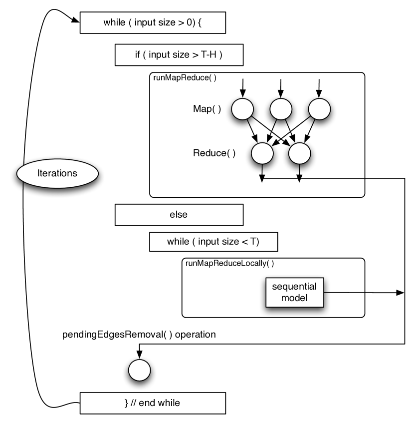
Figure 6: Hybrid Iterative MapReduce model

The original MapReduce model also permits one to define a Combine function that performs a sort of local reduce on each Map’s output, before the actual, distributed reduce phase. A Combine runs on the same machine as the related Map and it tries to partially aggregate intermediate data in order to improve the overall system performance. In our application we have chosen to discard this optimization because in TB nets context it is unlikely that symbolic states generated by the same parent have the same marking [3]. Thus, a combine phase before the reduce phase could even affect the performance of our application. By the way, using other formalisms this observation might be no more valid, and the Combine phase could be helpful.

Since the MapReduce model is not the best choice for elaborating a relatively small input, we introduced the possibility of changing the computational model, depending on the size of analyzed data set. Since the expansion front varies considerably during the $TRG$ building, it is convenient to use a sequential model on a single machine as long as it remains below a given threshold $T$. When the expansion front exceeds $T$, an Iterative MapReduce model on a large cluster of machines is employed. We call this approach (sketched in Fig. 6) Hybrid Iterative MapReduce (himapred). A hysteresis ($H$) is also programmed, in order to react with some delay in front of possible swings of the expansion front within $T$.

Fig. 7 shows the expansion front of the Gas Burner analysis over time. The trend line clearly shows how the execution time of a single MapReduce iteration depends on the $TRG$ size, denoted $|TRG|$. Since a Map processes a single sate, its execution time is independent from $|TRG|$ and in many cases it may be neglected. Conversely, a Reduce works on a partition of the $TRG$ (checking relationships between any pairs of nodes), thus its complexity is $O(|TRG|^{2})$. The worst case occurs when all nodes in the $TRG$ have the same feature $f(S)$: in that case a single Reduce has to process the whole graph. Although the worst case is very unlikely, a common situation is the presence of large clusters of nodes that share the same key $f(S)$. This leads to a computational load imbalance among the reducers often resulting in a significant degradation of performances.

Figure 7: Expansion front over time

V Experiments

The sequential builder produces a graph with 14563 nodes for the Gas Burner example (versus 23635 symbolic states generated during computation), and takes about 7.5 hours on a notebook with a 2.4Ghz Intel Core 2 Duo processor and 4GB of RAM (the operating system is Ubuntu 10.10 and the JVM is OpenJDK IcedTea6 1.9.5). In this paper we adopt the Gas Burner example as a well known benchmark and we are not interested in the properties of the system.

Testing activities on the JavaSpaces Tool have been performed on a local network (33 computers over a 100Mb Ethernet LAN). Preliminary experiments in this setting show that although performances are much better than for the single-thread program (the execution time is reduced by a factor $\sim 3.75$), there is a major bottleneck preventing further improvements: the state space partitioning among the Workers set is not uniform. This means that some computation units are much more loaded than others, which remain idle for most of the time. In order to alleviate this problem, we conceived a different partitioning policy that allows for a higher degree of parallelism. We used the function defined in (1) with a different $f$, called discriminant soft marking. Let $dm$ be a function:

$$\begin{split}dm:P\rightarrow\mathbb{N}^{2},~{}dm(p)=\langle i,j\rangle\end{split}$$ (4)

where $p$ is a place of the analyzed TB net, $j$ is the number of anonymous time-stamps in $p$, and $i$ is the number of other time-stamps in $p$. The discriminant soft marking of $S$ is now defined as:

$$\begin{split}f(S)=\langle dm(p_{1}),...,dm(p_{k})\rangle\,\in\mathbb{N}^{2k}\end{split}$$ (5)

This new definition comes from the observation that, even if two states have the same soft marking, according to (2), they cannot be included into one another if the distribution of anonymous time-stamps in the corresponding markings is different.

Fig. 8 shows the state space partitioning among 32 Worker processes using the two different partitioning policies. Table I reports the results of different experiments done within different settings.

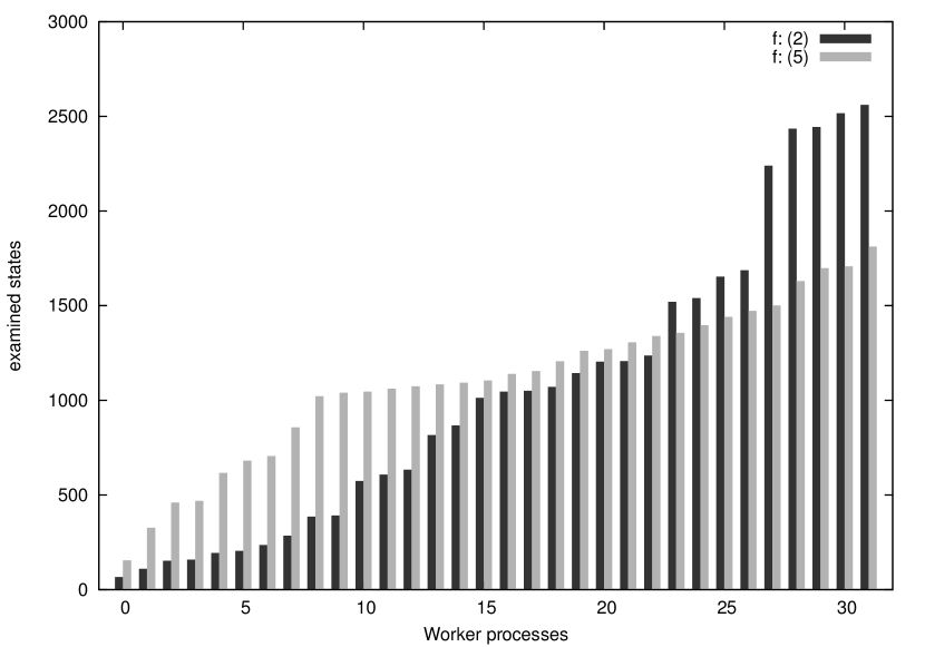
Figure 8: State space partitioning among 32 Workers

TABLE I: Experiments Report

architecture	$\#$ compute units	tool version	compute model	T	H	f	exec. time
2.4Ghz Intel Core 2 Duo, 2GB RAM	1 machine	sequential	local (single machine)	-	-	(2)	$\sim$7.5 hrs
3Ghz Intel Pentium 4, 2GB RAM	33 machines	JavaSpaces	local (distributed)	-	-	(2)	1h55m40s
3Ghz Intel Pentium 4, 2GB RAM	33 machines	JavaSpaces	local (distributed)	-	-	(5)	1h2m0s
m2.2xlarge [1]	39 ec2 units	himapred	cloud	200	50	(2)	1h35m33s
m1.xlarge [1]	104 ec2 units	himapred	cloud	200	50	(2)	1h43m19s
m2.2xlarge [1]	104 ec2 units	himapred	cloud	200	50	(2)	1h0m0s
m2.2xlarge [1]	104 ec2 units	himapred	cloud	400	100	(5)	46m8s
m2.2xlarge [1]	104 ec2 units	himapred	cloud	200	50	(5)	39m33s

The last MapReduce Tool has been deployed “in the cloud” by means of the Amazon Elastic MapReduce web service [1] that employs the Amazon Elastic Compute Cloud (EC2) infrastructure. Table  I summarizes the outcomes of the Gas Burner analysis carried out using different distributed frameworks with varying configurations. The results point out the different factors that contribute to improve the performances of our distributed applications: the number of computation units, the cluster dimension, the hardware of each cluster machine, and the partitioning policy. In particular the latter one shows to be a key factor for the possibility of conveniently scaling up the available computation resources.

VI Conclusion and future works

We have presented and discussed some approaches based on exploitation of distributed/cloud computing frameworks to deal with the state-space explosion in real time system analysis . These approaches have been experienced for timed (symbolic) reachability analysis of Time Basic (TB) Petri nets. The proposed implementations extend the sequential builder of TB nets’ time reachability graph. Standing on a common basic computational schema (a sort of Map & Fold), our approach is general enough to be used within different formalisms by specializing the $state$, the Map, the Reduce, and the $f$ concepts. In particular, we have designed and implemented an extension of the MapReduce model, called Hybrid Iterative MapReduce. The outcomes of tests performed on a benchmarking RT model clearly show how distributed (especially cloud) implementations can be conveniently used to increase the performances of the sequential builder. We plan to extend our research by trying to further refine the partitioning function and studying ways for integrating dynamic load balancing models not only into the JavaSpaces implementations but also into iterative MapReduce based computational frameworks, in order to cope with the main performance bottleneck.

Examples and binaries of the tools described in this paper can be found at: http://camilli.dico.unimi.it/graphgen with associated “how to install” notes.

References

- [1] Amazon Web Services LLC. Amazon Elastic MapReduce documentation. http://aws.amazon.com/documentation/elasticmapreduce/, 2012. Last visited: January 2012.
- [2] A. P. Atlee and H. Gannon. Specifying and verifying requirements of real-time systems. IEEE Trans. Softw. Eng., 19:41–55, January 1993.
- [3] Carlo Bellettini and Lorenzo Capra. Reachability analysis of time basic Petri nets: a time coverage approach. In Proc. of 13th International Symposium on Symbolic and Numeric Algorithms for Scientific Computing, SYNASC 2011, pages 110–117, Los Alamitos, CA, USA, 2011. IEEE Computer Society Press.
- [4] Carlo Bellettini, Miguel Felder, and Mauro Pezzè. A tool for analysing high-level timed Petri nets. IPTES Esprit Project 5570 PDM-41, Politecnico di Milano, September 1993.
- [5] Jeffrey Dean and Sanjay Ghemawat. MapReduce: simplified data processing on large clusters. Commun. ACM, 51:107–113, January 2008.
- [6] Jaliya Ekanayake, Hui Li, Bingjing Zhang, Thilina Gunarathne, Seung-Hee Bae, Judy Qiu, and Geoffrey Fox. Twister: a runtime for iterative MapReduce. In Proc. of Symposium on High Performance Distributed Computing, pages 810–818, 2010.
- [7] Eric Freeman, Ken Arnold, and Susanne Hupfer. JavaSpaces Principles, Patterns, and Practice. Addison-Wesley Longman Ltd., Essex, UK, UK, 1st edition, 1999.
- [8] Carlo A. Furia, Dino Mandrioli, Angelo Morzenti, and Matteo Rossi. Modeling time in computing: A taxonomy and a comparative survey. ACM Comput. Surv., 42:6:1–6:59, March 2010.
- [9] Hubert Garavel, Radu Mateescu, and Irina Smarandache. Parallel state space construction for model-checking. In Proceedings of the 8th international SPIN workshop on Model checking of software, SPIN ’01, pages 217–234, New York, NY, USA, 2001. Springer-Verlag New York, Inc.
- [10] David Gelernter and Nicholas Carriero. Coordination languages and their significance. Commun. ACM, 35:97–107, February 1992.
- [11] Carlo Ghezzi, Dino Mandrioli, Sandro Morasca, and Mauro Pezzè. A unified high-level Petri net formalism for time-critical systems. IEEE Trans. Softw. Eng., 17:160–172, February 1991.
- [12] The Apache Software Foundation. Hadoop MapReduce documentation. http://hadoop.apache.org/mapreduce/, 2007. Last visited: January 2012.
- [13] Antti Valmari. The state explosion problem. In Lectures on Petri Nets I, pages 429–528, London, UK, 1998. Springer-Verlag.