The onset of tree-like patterns in negative streamers

Abstract

We present the first analytical and numerical studies of the initial stage of the branching process based on an interface dynamics streamer model in the fully 3-D case. This model follows from fundamental considerations on charge production by impact ionization and balance laws, and leads to an equation for the evolution of the interface between ionized and non-ionized regions. We compare some experimental patterns with the numerically simulated ones, and give an explicit expression for the growth rate of harmonic modes associated with the perturbation of a symmetrically expanding discharge. By means of full numerical simulation, the splitting and formation of characteristic tree-like patterns of electric discharges is observed and described.

It is a well known visible fact that electric discharges form tree-like patterns, very much as those in coral reefs and snowflakes. The study of the branching process leading to such pattern is of considerable interest both from pure and applied points of view. Many industrial techniques, ranging from lasers to chemical processing of gases and water purification could be improved provided the development of tree-like patterns can be controlled or avoided. Although an electric discharge is a very complex phenomenon, with radiation and chemistry processes involved Rai ; Raether ; Pasko , the description of its initial stage is simpler. A single free electron traveling in a strong, uniform electric field ionizes the gaseous molecules around it, generating more electrons and starting a chain reaction of ionization. The ionized gas creates its own electric field, which speeds up the reaction, and a streamer is born. The streamers of ionized gas have an inevitable tendency to break up at their tips (see figure 1), followed by the creation of the familiar tree-like pattern .

Early efforts Dhali ; Vitello ; Lagarkov ; vanS were able to identify a minimal streamer model with which, after numerical simulations under the hypothesis of cylindrical symmetry, an instability was observed ME . Later on, the dispersion relation for planar fronts was computed and the existence of an instability leading to the development of fingers was found aftprl . Due to the enormous difficulty for performing full numerical simulations of the minimal streamer model, some simplified descriptions have been attempted in the last years (see ute2 for a review where various ad hoc assumptions are discussed). In any case, the fully 3-D case has resisted the attack so far. As an alternative approach (the one we follow in this work), the motion and propagation of the streamer discharge has recently been described by a contour dynamics model first introduced in Arrayas10 and used to predict with success some experimental features of discharges on dielectric surfaces Arrayas11 ; Japos . The contour dynamics model describes the interface separating a plasma region from a neutral gas region. For a negative discharge, the separating surface has a net charge $\sigma$ and the thickness goes to zero as $\sqrt{D}$, with $D$ the charge diffusion coefficient. The interface moves with a velocity in the normal direction

$$v_{N}=-\mu_{e}\mbox{E}_{\nu}^{+}+2\sqrt{\frac{D_{e}}{l_{0}}\mu_{e}|\mbox{E}_{\nu}^{+}|\exp\left(-\frac{\mbox{E}_{ion}}{|\mbox{E}_{\nu}^{+}|}\right)}-D_{e}\kappa,$$ (1)

where $\mbox{E}_{\nu}^{+}$ is the normal component of the electric field at the interface when approaching it from outside the plasma region, $\mu_{e}$ the electron mobility, $D_{e}$ is the electron diffusion coefficient, E_ion is a characteristic ionization electric field and $\kappa$ is twice the mean curvature of the interface. The parameter $l_{0}$ is the microscopic ionization characteristic length.

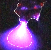
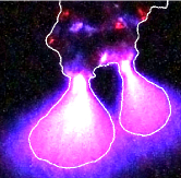
Figure 1: Experimental sequential images of the growth of a streamer in a corona discharge at its early stages. This is a 100 kV point-plane discharge in the vertical direction with an air-gap of 30 cm. The contour has been highlighted as a visual aid.

The total negative surface charge density at the interface changes according to

$$\frac{\partial\sigma_{e}}{\partial t}+\kappa v_{N}\sigma_{e}=-\frac{\mbox{E}_{\nu}^{-}}{\varrho_{e}}-j_{\nu}^{-}\,,$$ (2)

where $\mbox{E}_{\nu}^{-}$ is the electric field at the interface coming from inside the plasma, $\varrho_{e}$ is a parameter proportional to the resistivity of the electrons in the created plasma and $j_{\nu}^{-}$ is the current contribution at the surface of any source inside the plasma. For instance, an insulated wire inside the plasma at $\mathbf{x}_{0}$, carrying an electric current $I(t)$, will create a current density inside the plasma and as quasineutrality is fulfilled, we will have for the plasma region

$$\nabla\cdot\mathbf{j}=I(t)\delta(\mathbf{x}-\mathbf{x}_{0})$$ (3)

and $\mathbf{j}$ is obtained solving that equation. Note that at the interface there is an electric field discontinuity given by

$$\mbox{E}_{\nu}^{+}-\mbox{E}_{\nu}^{-}=-\frac{e\sigma}{\varepsilon_{0}}.$$ (4)

It is convenient to express the model in dimensionless units. The physical scales are given by the ionization length $l_{0}$, the characteristic impact ionization field $\mbox{E}_{i}$, and the electron mobility $\mu_{e}$. The velocity scale yields $U_{0}=\mu_{e}\mbox{E}_{i}$, and the time scale $\tau_{0}=l_{0}/U_{0}$. Typical values of these quantities for nitrogen at normal conditions are $l_{0}\approx 2.3\,\mu\mathrm{m}$, $\mbox{E}_{i}\approx 200$ kV/m, and $\mu_{e}\approx 380\,\mathrm{cm^{2}/Vs}$. The unit for the negative surface density reads $\sigma_{0}=\varepsilon_{0}{\mbox{E}}_{i}/e$, so for the current density $j_{0}=\sigma_{0}U_{0}/l_{0}$ and for the resistivity $\varrho_{0}=\mu_{e}l_{0}/\sigma_{0}$. The diffusion constant unit turns out $D_{0}=l_{0}U_{0}$. Introducing dimensionless units, the model reads

$$v_{N}=-\mbox{E}_{\nu}^{+}+2\sqrt{\varepsilon\alpha(|\mbox{E}_{\nu}^{+}|)}-\varepsilon\kappa,$$ (5)

$$\frac{\partial\sigma}{\partial t}+\kappa v_{N}\sigma=-\frac{\mbox{E}_{\nu}^{-}}{\varrho}-j_{\nu}^{-}\,,$$ (6)

being

$$\alpha(|\mbox{E}_{\nu}^{+}|)=|\mbox{E}_{\nu}^{+}|\exp\left(-\frac{1}{|\mbox{E}_{\nu}^{+}|}\right),$$ (7)

and $\varepsilon=D_{e}/D_{0}$ the dimensionless diffusion coefficient. In what follows all the quantities are dimensionless unless otherwise indicated. We have used an adaptive boundary element method, developed for general contour dynamics problems (font1 ; font2 ) in order to perform numerical simulations with equations (5) and (6).

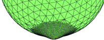
(a) Initial configuration

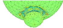
(b) $t=0.0794$

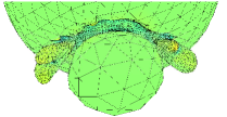
(c) $t=0.1438$

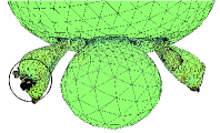
(d) $t=0.1769$. The encircled region is enlarged in figure 3

Figure 2: Evolution of the plasma for $Q=-25$, $E=0.5$ and $\varepsilon=0.02$. Color gradation represents curvature.

In figure 2 we show numerical simulations of the evolution of the discharge at four time steps. The plasma is assumed ideally conducting, initially charged with integrated surface charge Q=-25, subject to an external field in the vertical direction $E=0.5$, and confined inside an initially spherical geometry perturbed by $r_{0}(\theta,\phi)=R_{0}+\delta_{0}(\exp(-(\cos^{2}(\phi)+\cos^{2}(\theta))/c)$, with $c=0.03$ and $\delta_{0}=0.1$. We first observe the onset of streamer fingers. At time t = 0.17 the streamers develop further instabilities and split again. Qualitatively the process can be described in the following terms: any protuberance that develops is accompanied by an increase of the charge density at its tip. The electrostatic repulsion of charges at the tip tends to make the tip expand and the finger grow. In opposition to this is the action of the surface tension tending to flatten the protuberance and setting up a flux of charge from the protuberance out to the sides. However, overall, the protuberance becomes amplified. This process occurs again and again until a tree-like pattern is produced. In figure 3 we depict a detail of this pattern. Those ideas where anticipated in ME , but due to the restriction of 2-D simulations the whole process of the branching pattern formation could not be observed.

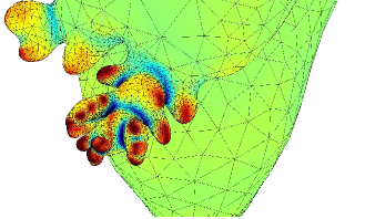
Figure 3: Detail of the shape of the plasma at $t=0.1769$

In order to be quantitative, we can calculate the growth rate of the different modes, both analytically and numerically. If the initial spherical symmetry is perturbed by a small amount, some instabilities will start growing. We will study which instability modes are going to prevail during the front evolution.

We consider now a spherically expanding plasma, representing a corona discharge, with ${Q(t)}<0$ so that $E_{0}=\mbox{E}_{\nu}^{+}=\frac{Q(t)}{4\pi R(t)^{2}}<0$. Then, $R(t)$ is given as the solution of

$$\frac{dR}{dt}=-\left(\frac{Q(t)}{4\pi R}+2\varepsilon\right)\frac{1}{R}+2\varepsilon^{\frac{1}{2}}\sqrt{\alpha(|\mbox{E}_{\nu}^{+}|)}.$$ (8)

If $Q(t)=Q$ it is easy to check that

$$R(t)\approx\left(\frac{3\left|Q\right|}{4\pi}t\right)^{\frac{1}{3}},$$ (9)

for the early stages of the discharge and as long as $R\quad\ll\frac{|Q|}{\varepsilon}$. This is in agreement with predictions based on continuum streamer models aft1 ,r3 . If the position of the front as well as the charge density are changed by a small amount, the perturbed quantities can be parameterized as

$$r(\theta,\phi,t) = R(t)+\delta S(\theta,\phi,t),$$ (10)

$$\sigma(\theta,\phi,t) = -\frac{Q(t)}{4\pi R^{2}(\theta,\phi,t)}+\delta\Sigma(\theta,\phi,t),$$ (11)

where $\delta$ is a small parameter. The angles $\theta$, and $\phi$ are the usual spherical coordinates. For convenience we write the surface perturbation in terms of spherical harmonics as

$$S=\sum_{l=1}^{\infty}\sum_{m=-l}^{l}s_{lm}(t)Y_{lm}(\theta,\phi),$$ (12)

and the surface charge density perturbation as

$$\Sigma=-\sum_{l=1}^{\infty}\sum_{m=-l}^{l}\left(\frac{2l+1}{R}\,b_{lm}+\frac{Q(t)}{4\pi R^{2}}\frac{l+1}{R}\,s_{lm}\right)Y_{lm}(\theta,\phi)$$ (13)

where the coefficients $s_{lm}(t)$ and $b_{lm}$ have to be determined. Making a standard expansion of the dynamics contour model equations (5) and (6), up to linear terms, we get the equations for the particular mode evolution

$$\begin{split}\frac{ds_{lm}}{dt}&=\Biggl{[}\varepsilon^{\frac{1}{2}}\frac{\sqrt{\alpha_{0}}\,\mathrm{sign}(Q(t))}{|E_{0}|}\biggl{(}1+\frac{1}{|E_{0}|}\biggr{)}-1\Biggr{]}\frac{(l+1)}{R}\,b_{lm}\\ &+\Biggl{[}\varepsilon^{\frac{1}{2}}\sqrt{\alpha_{0}}\left(1+\frac{1}{|E_{0}|}\right)-E_{0}-\frac{\varepsilon(l+2)}{R}\Biggr{]}\frac{(l-1)}{R}\,s_{lm},\end{split}$$ (14)

$$\begin{split}&\frac{db_{lm}}{dt}=\frac{(l^{2}-1)E_{0}}{(2l+1)R}\left[2E_{0}+\frac{(l+4)\varepsilon}{R}-(\varepsilon\alpha_{0})^{\frac{1}{2}}\,\biggl{(}3+\frac{1}{|E_{0}|}\biggr{)}\right]s_{lm}\\ &-\frac{I(t)(l+1)}{4\pi R^{2}(2l+1)}s_{lm}+\Big{[}\frac{(l^{2}+4l+2)}{(2l+1)}E_{0}+\frac{2\varepsilon}{R}\\ &-\varepsilon^{\frac{1}{2}}\frac{\sqrt{\alpha_{0}}}{(2l+1)}\biggl{(}l^{2}+6l+3+\frac{(l+1)^{2}}{|E_{0}|}\biggr{)}-\frac{lR}{(2l+1)\varrho}\Big{]}\frac{b_{lm}}{R}.\end{split}$$ (15)

We can get information about the growth of different modes by analyzing two special limits. First we study the limit of ideal conductivity. It corresponds to $\varrho\rightarrow 0$, and hence, from (LABEL:eqblm), we can conclude that $b_{lm}\rightarrow 0$. This is the case when in the limit of very high conductivity, the electric field inside goes to zero ($E_{\nu}^{-}\rightarrow 0$), as we approach to the behavior of a perfect conductor. If we consider that $Q(t)=Q_{0}$ is constant or its variation in time is small compared with the evolution of the modes (which also implies $I(t)\rightarrow 0$), and the same for the radius of the front $R(t)=r_{0}$, we look for a solution $s_{lm}=\exp(\omega t),\,\varphi_{n}=0$, to (14), and get a discrete dispersion relation of the form

$$\omega=\Biggl{[}\varepsilon^{\frac{1}{2}}\sqrt{\alpha_{0}}\left(1+\frac{1}{|E_{0}|}\right)-E_{0}-\frac{\varepsilon(l+2)}{r_{0}}\Biggr{]}\frac{(l-1)}{r_{0}},$$ (16)

with a maximum at

$$l=l_{max}\simeq\frac{|E_{0}|r_{0}}{2\varepsilon},$$ (17)

for $\varepsilon\ll 1$. For a small enough conductivity, $\varrho\rightarrow\infty$, we find $b_{lm}=-E_{0}s_{lm}(l+1)/(2l+1)$, and with $s_{lm}=\exp(\omega t)$, (14) yields

$$\omega=\Biggl{[}\varepsilon^{\frac{1}{2}}\sqrt{\alpha}_{0}\,\biggl{(}1+\frac{1}{|E_{0}|}\biggr{)}-E_{0}\Biggr{]}\frac{(l^{2}-3l-2)}{(2l+1)r_{0}}-\frac{\varepsilon(l+2)(l-1)}{r_{0}^{2}},$$ (18)

with a maximum at

$$l=l_{max}\simeq\frac{|E_{0}|r_{0}}{\varepsilon},$$ (19)

for $\varepsilon\ll 1$. Note that the dispersion relation does not depend on $m$. The finite resistivity cases lay between those limits. In fig 4 we have plotted the analytical curves given by (16) for different values of $\varepsilon$ and the results of numerical calculations for a perfect conductor.

Figure 4: Analytical (in black) and numerical dispersion curves for different values of the diffusion coefficient $\varepsilon$. The abscissa corresponds to the spherical harmonics number, and the ordinate to the growth rate for that mode.

The dispersion curve allows to predict the expected number of branches that will develop. Each branch will undergo also a further split and so on propagating to the smaller scales. However, it cannot run forever, as there is a limitation and the model does not take into account the energy radiated, the heat exchange, and the other phenomena that will start to play an important role at later stages of the discharge.

The results presented in this work confirm the hypothesis that at the earlier stages of an electric discharge, the main driving forces are diffusion and electrical drift, first anticipated in ME . The expressions obtained for the growth rate of the modes, given by (16) and (18) enables one to predict the number of forks that one can expect in an electric discharge provided the electric field and the diffusion constant is known by other means. But, the opposite can be worked out: from the numbers of fingers observed, we can for example infer the electric field if the charge density at the interface and the diffusion constant are known. This has been done for the 2-D case Arrayas11 . For the 3-D case, the density can be obtained from Stark’s effect measurements, and effective diffusion coefficient may be approximately calculated. These results contribute to achieve one of the main goals, both in the laboratory and in nature, of the current research in the area of electric discharges: bringing the field from a qualitative and descriptive era to a quantitative one.

Acknowledgments. This work has been supported by the Spanish Ministerio de Ciencia e Innovación under projects AYA2009-14027-C07-04, AYA2011-29336-C05-03 and MTM2011-26016.

References

- (1) Y. P. Raizer, Gas Discharge Physics (Springer, Berlin 1991).
- (2) H. Raether, Electron avalanches and Breakdown in gases (Butterworths, London, 1964).
- (3) V. P. Pasko, Nature, 423, pp. 927-929, 2003.
- (4) S. K. Dhali and P. F. Williams, Phys. Rev. A 31, 1219 (1985); J. Appl. Phys. 62, 4696 (1987).
- (5) P. A. Vitello, B. M. Penetrante and J. N. Bardsley, Phys. Rev. E 49, 5574 (1994).
- (6) A. N. Lagarkov and I. M. Rutkevich, Ionization waves in electric breakdown on gases (Springer-Verlag, New York, 1994).
- (7) U. Ebert, W. van Saarloos and C. Caroli, Phys. Rev. Lett. 77, 4178 (1996); Phys. Rev. E 55, 1530 (1997).
- (8) M. Arrayás, U. Ebert and W. Hundsdorfer, Phys. Rev. Lett. 88, 174502 (2002).
- (9) M. Arrayás, M. A. Fontelos and J. L. Trueba, Phys. Rev. Lett. 95, 165001 (2005). U.
- (10) U. Ebert et al. Nonlinearity 24, C1-C26 (2011).
- (11) M. Arrayás, M. A. Fontelos and C. Jiménez, Phys. Rev. E 81, 035401(R) (2010).
- (12) M. Arrayás and M. A. Fontelos, Phys. Rev. E 84, 026404 (2011).
- (13) D. Tanaka et al. J. Phys. D: Appl. Phys. 42, 075204 (2009).
- (14) Arrayás, M., Fontelos, M.A. & Trueba, J.L., Phys. Rev. E 71, 037401 (2005).
- (15) Kyuregyan, A. S, Phys. Rev. Lett. 101, 174505 (2008)
- (16) M. A. Fontelos, V.J. García-Garrido and U. Kindelán, SIAM J. Appl. Math. Volume 71, No. 6, pp. 1941 - 1964 (2011).
- (17) M. A. Fontelos, U. Kindelán, O. Vantzos, Phys. Fluids 20, 092110 (2008).