Generating non-Gaussian states using collisions between Rydberg polaritons

Abstract

We investigate theoretically the deterministic generation of quantum states with negative Wigner functions, by using giant non-linearities due to collisional interactions between Rydberg polaritons. The state resulting from the polariton interactions may be transferred with high fidelity into a photonic state, which can be analyzed using homodyne detection followed by quantum tomography. Besides generating highly non-classical states of the light, this method can also provide a very sensitive probe for the physics of the collisions involving Rydberg states.

The generation and characterization of highly non-classical states of the light have accomplished considerable progress during recent years. This includes for instance the production and analysis of one- Hansen and two- Ourj2 ; Val photon Fock states, and of superpositions of coherent states, often called “Schrödinger’s cat” states cats . In these experiments, the desired states are obtained by using so-called “measurement-induced non-linearities”, where a measurement is performed on one part of an entangled state. Then the other part is projected onto the desired state, conditional to obtaining the good result in the projecting measurement. This method works quite well, but it is intrinsically non-deterministic : the probability of success is usually low, and the desired state cannot be created “on demand”, when needed for applications e.g. for quantum communications.

Here we would like to investigate another scheme, which can, at least in principle, be made more deterministic, by using Rydberg interactions in a cold atomic gas. Rydberg states are highly excited atomic states, that interact very strongly at distances $R$ of order a few $\mu$m, through either dipole-dipole ($1/R^{3}$) or van der Waals ($1/R^{6}$) interactions Ry ; rydbergs . The idea is first to change a generic photonic state, for instance a weak coherent state, into a so-called “polariton” state, where a long-lived excitation is distributed over many atoms EIT . Here we will consider Rydberg polariton states, where many atoms share a few delocalized Rydberg excitations Ry . The prepared polariton state will then evolve under the action of these Rydberg-Rydberg interactions, generating highly non-classical (typically non-Gaussian) states kuzmich . When the desired state is obtained, the polariton state can be converted back into a free-propagating photonic state, using a control laser beam (see Fig. 1). The phase-matching condition between the input, write, read, and signal beams leads to a collective enhancement effect ensuring that the state of the light is emitted in a well-defined spatial and temporal mode Bariani . The conversion of the polariton state back to photons is then expected to deterministically produce highly non classical states Gorshkov07 ; Vuletic ; Gorshkov11 ; us . In addition, the analysis of the generated state will give information about the collisional mechanisms which take place between the Rydberg atoms.

Let us emphasize that a particularly useful method to fully characterize highly non-classical states is quantum tomography, which allows one to reconstruct the Wigner function $W(q,p)$ of the state in phase space, where $\hat{q}$ and $\hat{p}$ are the quadrature operators of the quantized electric field, measured using homodyne detection Hansen ; Ourj2 ; Val ; cats . Such a method provides a full characterization of the measured quantum state, which is very intuitive because the “non-classicality” of the measured state, and especially its purity, directly translate into the negativity of the Wigner function Barbieri . We will thus use such Wigner functions to characterize both the photon and the polariton states.

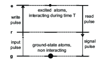
Figure 1: An ensemble of $N$ three-level atoms is initially prepared in a coherent Rydberg polariton state, with only a few atoms excited. After a time shorter than the decoherence time, the collisions have modified in a non-linear way the coefficients of the polariton state, which is “remapped” onto a photonic state, and analyzed using an homodyne detection.

In this letter we will study the first two steps of such a deterministic preparation of non-Gaussian states :

(i) preparing the coherent polariton state using a weak laser pulse; we will introduce the phase-matched symmetric Dicke states pillet as a convenient way to describe the states of the ground and excited atoms (this is essentially equivalent to the polariton picture EIT ).

(ii) leaving the polariton state evolve for some time (shorter than its decoherence time). The state will then be modified in a non-linear way, depending on the nature of the Rydberg-Rydberg interactions. We will obtain simple analytic expressions for this evolution, that are the main results of the present paper.

Finally, we will characterize the generated polariton states by computing their Wigner functions, and we will discuss various experimental considerations, including the remapping of the polariton into a photonic state.

The calculation is performed by splitting the evolution of the system in two steps : first, an excitation step using a short (typically $\sim$ 1 ns) and weak laser excitation pulse, creating a few Rydberg states; second, a free evolution of the generated state under the effect of Rydberg-Rydberg interactions. We will show that we can consistently ignore the interactions during the first step, and then ignore the laser in the second step, since it is turned off.

In order to describe the excitation step for an ensemble of $N$ atoms from a ground state $g$, we consider a two–photon excitation, off-resonant from the intermediate level $r$, and resonant with the Rydberg state $e$ (see Fig. 1). It can thus be described using an effective two-level model rydbergs with the Hamiltonian $H=H_{\ell}+H_{c}$, where

$$H_{\ell}=\frac{\hbar\Omega(t)}{2}\sum\limits_{i=1}^{N}\left({\hat{\sigma}_{eg}^{i}+\hat{\sigma}_{ge}^{i}}\right),\;\;H_{c}=\sum\limits_{i=1,j>i}^{N}{\hbar\kappa_{ij}}\hat{\sigma}_{ee}^{i}\hat{\sigma}_{ee}^{j}.$$

Here $\hat{\sigma}_{\alpha\beta}^{i}=\left|\alpha\right>\left<\beta\right|\mathrm{e}^{\pm(1-\delta_{\alpha\beta})i\vec{k}.\vec{R_{i}}}$, $\vec{R_{i}}$ is the position of atom $i$, and $\vec{k}$ the total wave-vector of the exciting light, with an effective (pulsed) Rabi frequency $\Omega(t)$; $\hbar\kappa_{ij}$ is the pair-wise interaction energy of the excited atoms, and $\delta_{\alpha\beta}$ the Kronecker symbol.

For short times and very low excitation fractions, let us first neglect the interaction term $H_{c}$ and keep only the laser excitation $H_{\ell}$. The result of laser excitation is then a coherent polariton state, that is a superposition of symmetric “phase-matched” Dicke states $\left|n\right>$, where $n$ is the number of excited atoms (see Appendix 1). The amplitude $C_{n}$ corresponding to the collective states $\left|n\right>$ directly follows from the single-atom amplitudes

$$C_{n}=(-i)^{n}\sqrt{B(N,n)}\sin^{n}\frac{\omega}{2}\cos^{N-n}\frac{\omega}{2},$$ (1)

where $B(N,n)$ is the binomial coefficient, $N$ is the total number of atoms and $\omega=\int\Omega(t)dt$ is the pulse area. In the limit of very small $n/N$, one has

$$\lim_{n/N\rightarrow 0}C_{n}/C_{n-1}=\alpha/\sqrt{n},$$ (2)

where $\alpha=-i\sqrt{N}\tan(\omega/2)\approx-i\sqrt{N}\omega/2$. The amplitude $\alpha$ is related to the averaged number of excited atoms $\langle N_{\rm exc}\rangle=N\omega^{2}/4=|\alpha|^{2}$. Relations (2) yields the well known expression $C_{n}/C_{0}=\alpha^{n}/\sqrt{n!}$ for the amplitudes of a coherent state, with $C_{0}$ determined by normalization. For this calculation to be consistent, we need to fulfill the condition $\langle n|\exp{(-iH_{c}\tau/\hbar)}|n\rangle\sim 1$ at the end of the laser pulse of duration $\tau$, where $H_{c}$ is the collisional part of the Hamiltonian; this will be checked in Appendix 2.

After the laser pulse is off, we consider the evolution of the previous coherent Rydberg polariton state under the only action of the Rydberg interaction Hamiltonian $H_{c}$. A crucial remark is that during the excitation and de-excitation phases (see Fig. 1), only the the symmetric phase-matched Dicke states (see Appendix 1) will be mapped coherently between the polariton and photonic states EIT . In addition, the Hamiltonian $H_{c}$ preserves the number of excitations $n$, and therefore it only mixes symmetric Dicke states with non-symmetric ones, which are uncoupled from the laser readout process.

In order to characterize the phase-matched part of the state after an evolution time $T$, we need therefore to evaluate the matrix elements $\langle n|U|n\rangle$, where $U=\mathrm{e}^{-iH_{c}T/\hbar}$. For this purpose we use the following transformation

$$e^{-i\kappa_{pq}T\,\hat{\sigma}^{i_{p}}_{ee}\hat{\sigma}^{i_{q}}_{ee}}=1+\hat{\sigma}^{i_{p}}_{ee}\hat{\sigma}^{i_{q}}_{ee}\left(e^{-i\kappa_{pq}T}-1\right).$$ (3)

For a low number of excited atoms, the probability to have $p$ interacting atoms close to each other vanishes very quickly as $p$ increases. Therefore, the leading interaction order originates from two-body interactions, the next-to-leading order originates from three-body interactions and so forth. The transformation (3) can facilitate this expansion because the term $(e^{-i\kappa_{pq}T}-1)$ is zero if the two atoms do not interact, i.e. if they are far from each other. One can then use these types of terms to select pairs of interacting atoms in various interaction orders, and the expectation values $\langle n|U|n\rangle$ can be evaluated by bookkeeping various combinations and contributions of $p$ excited atoms, with $p\leq n$. The expansion is finite (since $p\!\leq\!n$), however the number of terms and their complexity rapidly increase for $p\geq 4$; we will therefore look first at low $n$, and then find an excellent ansatz for higher $n$.

Denoting as $\eta({\bf r})$ the atom number density at point $\bf r$, and $dN_{i}=d^{3}r_{i}\;\eta({\bf r_{i}})$, we define :

$$I_{2}\!=\!\frac{1}{N^{2}}\iint dN_{i}\;dN_{j}\;(e^{-i\kappa_{ij}T}-1),$$ (4)

$$J_{3}\!=\!\frac{1}{N^{3}}\iiint dN_{i}\;dN_{j}\;dN_{s}\times$$

$$\hskip 19.91692pt(e^{-i\kappa_{ij}T}-1)(e^{-i\kappa_{is}T}-1),$$ (5)

$$I_{3}\!=\!\frac{1}{N^{3}}\iiint dN_{i}\;dN_{j}\;dN_{s}\times$$

$$\hskip 19.91692pt(e^{-i\kappa_{ij}T}-1)(e^{-i\kappa_{is}T}-1)(e^{-i\kappa_{js}T}-1),$$ (6)

and one gets the successive terms

$$\langle 0|U|0\rangle\! = \!\langle 1|U|1\rangle=1,$$

$$\langle 2|U|2\rangle\! = \!1+I_{2},$$

$$\langle 3|U|3\rangle\! = \!1+3I_{2}+3J_{3}+\;I_{3},$$

$$\langle n|U|n\rangle\! = \!1+B(n,2)I_{2}+3B(n,3)J_{3}+\;B(n,3)I_{3}+\ldots$$

For each $\langle n|U|n\rangle$, the coefficients of the quantities $I_{2,3}$ and $J_{3}$ correspond to the numbers of different choices of excited atoms $(i,j)$ and $(i,j,s)$ that appear in the expressions (4)-(6). Though this approach is rigorous and can work in principle at any order, it has the disadvantage that the integrals $I_{n}$ are more and more complicated to evaluate when $n$ increases. Whereas $I_{2}$ can easily be calculated analytically (see Appendix 3), this is more tedious for $I_{3}$, and $I_{n>3}$ are only numerical. We therefore introduce now a much simpler approach, giving analytical results at any order, which works surprisingly well when compared with numerical calculations.

The idea is to evaluate $U_{n>m}\,$, assuming that $U_{m}\!=\!\langle m|U|m\rangle$ is known. For this purpose, we first note that the value of $U_{n}$ for a set $\{n\}=\{i_{1},\;i_{2},\;...\;i_{n}\}$ of $n$ excited atoms can be formally divided into a product of terms involving set $\{m\}$ of $m<n$ atoms, in the following way (we note that the total number of excited atoms is always conserved) :

$$\left\langle\exp(-iK_{c})\right\rangle_{\{n\}}\!\!=\!\!\prod\limits_{i_{1}<...<i_{m}\atop i_{m}\leq i_{n}}\!\!\!\bigg{\langle}\!\exp(-i\lambda_{nm}K_{c})\!\bigg{\rangle}_{\{m\}}$$ (7)

where $K_{c}=H_{c}T/\hbar$, and $\lambda_{nm}\!\!=\!B(n,2)/[B(n,m)B(m,2)]$ is due to the fact that each $\kappa_{ij}$ appears in several subsets.

We also note that the calculation of $U_{m}$ for a given set $\{n\}$ of atoms will involve an average over all random positions of atoms, that is essentially the continuum limit of the above expressions. Taking into account this averaging, the quantities $\langle\exp(-i\lambda_{nm}K_{c})\rangle_{\{m\}}$ are the same for all $m$-subsets. As a consequence, we use as a crucial ansatz that the rhs of Eq. (7) is just a product of $B(n,m)$ identical factors $\langle\exp(-i\lambda_{nm}K_{c})\rangle_{\{m\}}$ :

$$\langle n|U|n\rangle\! = \!\left\langle\exp(-iK_{c})\right\rangle_{\{n\}}$$ (8)

$$\approx \,\langle\exp(-iK_{c})\rangle_{\{m\}}^{B(n,m)\lambda_{nm}}\!=\!\langle m|U|m\rangle^{\frac{n(n-1)}{m(m-1)}}\;\;\;\;\;.$$

For $m\!=\!2$, one has then simply:

$$\langle n|U|n\rangle=(1+I_{2}(T))^{n(n-1)/2}$$ (9)

where $I_{2}(T)$ can be calculated analytically by integrating on the positions of two atoms within a sphere of constant atomic density, the result is given in Appendix 3.

Figure 2 shows the plots of $\langle n|U|n\rangle$, $n$ = 2, 3 and 4 for van der Waals interactions, as a function of the scaled interaction time $t$. For each $n$ three different curves are almost perfectly overlapping : the green dotted curves are the numerical results, the red full ones show the scaling from $n=2$ using the expression of $I_{2}(t)$ given in Appendix 3, and the blue dashed ones show the scaling from $n=3$. In the numerical calculation, groups of four atoms are generated and $\langle n|U|n\rangle$ is essentially the averaged $U$ over random n-groups of atoms. The calculations are done for a sphere with a uniform density, but can be generalized for arbitrary density profiles.

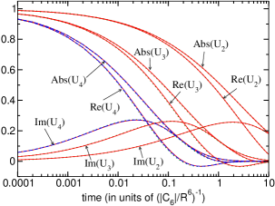
Figure 2: Real and imaginary parts, and modulus of $U_{m}\!=\!\langle m|U|m\rangle$ as a function of time in units of $T_{R}=R^{6}/|C_{6}|$, for attractive van der Waals interactions. For repulsive interactions one has only to change the sign of ${\rm Im}(U_{n})$. All red curves are obtained by scaling from the corresponding $U_{2}$ using Eq. (9). All blue dashed lines are obtained using the scaling formula (8) with the exact numerical result for $U_{3}$, and all green dotted lines are the results of the full numerical calculation. Similar results (not shown here) can be obtained for dipole-dipole interactions rather than Van der Waals interactions.

Summarizing, we have thus obtained a series of simple approximate expressions of $\langle n|U|n\rangle$, valid for any $n$. This surprisingly simple derivation can be understood as an approximate but efficient way to resum the terms appearing in the more rigorous expansion quoted before.

In order to analyze the generated polariton states, it is convenient to use Wigner functions, that show the evolution of the initial Gaussian into non-Gaussian states. Simple analytical calculations give easily $W(q,p)$ in a suitably truncated Fock state basis, as a function of the coefficients $\langle n|\hat{\rho}|m\rangle$ of the density matrix, obtained from the evolution of the initial Dicke state using previous formulas. For long interaction times, the result is rather simple : since the coefficients for $n=0$ and 1 are unaffected, and all other ones go to zero, the Rydberg medium behaves as deterministic near-perfect “quantum scissors” qs , cutting the initial coherent state into the subspace of Fock states with zero and one photon :

$$|\alpha\rangle\rightarrow|0\rangle+\alpha|1\rangle$$

This is in agreement with the recent result of Kuzmich et al. kuzmich . In addition, we have the explicit expressions to calculate the evolution between the initial Gaussian coherent state, and the final truncated non-Gaussian state, as illustrated on Fig. 3.

As an exemple of realistic experimental parameters, let us consider 2500 atoms in a sphere of radius $R$ = 10 $\mu$m so $n_{at}=6\;10^{11}$ cm^-3. For the (repulsive) 70s state of Rb⁸⁷, one has $|C_{6}|/(2\pi)$ = 880 GHz $\mu m^{6}$ RR , so the time scaling is $T_{R}=R^{6}/|C_{6}|$ = 180 ns. An initial coherent state with amplitude $|\alpha|\sim 1$, excited by a pulse of duration 0.72 ns ($0.004\,T_{R}$) will evolve into a non-Gaussian state within a time of 720 ns ($4\,T_{R}$), as shown on Fig. 3. If the atoms are inside a low-finesse optical cavity, these numbers also warrant a large cooperativity parameter C with high outcoupling mirror transmission $T_{c}$ ($C\sim 180$ for $T_{c}=0.01$), which should in turn warrant a good recovery of the photonic state Gorshkov07 ; Vuletic ; us .

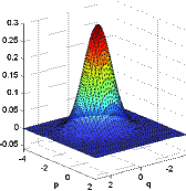
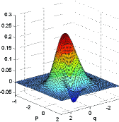
Figure 3: Evolution of the Wigner function of an initial coherent state $|\alpha\rangle$ with $|\alpha|=1$, between the scaled times 0.004 (left side) and 4 (right side), that is close to the truncated state $|0\rangle+\alpha|1\rangle$. The corresponding physical times are 0.72 ns (left) and 720 ns (right), with Van der Waals interactions only.

As a conclusion, we have studied the evolution of a coherent (Dicke) Rydberg polariton state, under the effect of Rydberg-Rydberg collisions. The non-linearities are clearly large enough to have an effect at the few-photon level, even outside the dipole blockade range. They are able to turn an input coherent state into a non-Gaussian state, at the expense of significant losses due to the decoherence of states containing more that one polariton. Whether or not such decoherence effects can be avoided in order to reach a high input-output recovery of photonic states is still an open question. Let us emphasize however that this decoherence does not prevent the polariton state, once created, to be remapped with high efficiency on a photonic state, and then analyzed using an homodyne detection us . This may also provide an interesting way to investigate Rydberg-Rydberg collisions.

Appendix

(A1) The Dicke state $|n\rangle$ corresponding to $n$ excited atoms among $N$ atoms is defined as the eigenstate with eigenvalues ($n-N/2$, $r(r+1)$) of the operators ($\hat{J}_{\vec{k}}^{(z)}$, $\hat{J}_{\overrightarrow{k}}^{2}$), with $\hat{J}_{\vec{k}}^{(z)}=\sum_{i=1}^{N}(|e,i\rangle\langle e,i|-|g,i\rangle\langle g,i|)/2$, $\hat{J}_{\vec{k}}^{(+)}=\sum_{i=1}^{N}|e,i\rangle\langle g,i|\exp(i\vec{k}.\vec{R_{i}})$, $\hat{J}_{\vec{k}}^{(-)}=(\hat{J}_{\vec{k}}^{(+)})^{\dagger}$ and $\hat{J}_{\vec{k}}^{2}=(\hat{J}_{\vec{k}}^{(+)}\hat{J}_{\vec{k}}^{(-)}+\hat{J}_{\vec{k}}^{(-)}\hat{J}_{\vec{k}}^{(+)})/2+(\hat{J}_{\vec{k}}^{(z)})^{2}$, where $\vec{R_{i}}$ is the position of atom $i$, and $\vec{k}$ is the total wave-vector of the exciting light. Symmetric Dicke states are obtained for $r=N/2$, and non-symmetric ones for $r\leq N/2-1$.

(A2) To estimate the action of the collisions during the short excitation phase of duration $\tau$, two points must be considered. The first one is that the excitation of a Rydberg atom creates a “blockade sphere” around it, where a second atom cannot be excited. The second one is that the quantities $U_{n}$ calculated above should remain close to one during $\tau$, so that the excitation and the collisions act on different time scales. To evaluate the first correction we can use the following correlation function $G_{ij}$ derived in jovica2010 for two level atoms and small $\omega$

$$G_{ij}\equiv\frac{\langle\hat{\sigma}^{i}_{ee}\hat{\sigma}^{j}_{ee}\rangle}{\langle\hat{\sigma}^{i}_{ee}\rangle\langle\hat{\sigma}^{j}_{ee}\rangle}=\frac{4\left|\int_{t_{0}}^{\tau}dt_{1}\,e^{i\kappa_{ij}t_{1}}\Omega(t_{1})\omega(t_{1})\right|^{2}}{|\omega(\tau)|^{4}}.$$ (10)

This function prevents two excited atoms to be closer to each other than a distance $r_{b}$ with magnitude given by $C_{6}\tau/r_{b}^{6}\sim 1$, where $\tau$ is the duration of the excitation pulse. It is thus clear that $r_{b}$ will be small if $\tau$ is small. More quantitatively, the modification of Eq. (9) would be to substitute $I_{2}(T)$ by $c(\tau,T)I_{2}(T)$, where $c(\tau,T)$ is a correction factor evaluated numerically. For the parameters quoted in the text, we numerically get $c(\tau,\tau)\!\approx\!0.984\!$ at the end of the excitation pulse, and this effect is thus negligible. Similarly, using the results in Appendix 3 one gets for $t=\tau/T_{R}$ = 0.004 the values $U_{2}\approx 0.94+0.05\,i$, $U_{3}\approx 0.82+0.13\,i$, $U_{4}\approx 0.66+0.21\,i$, that is acceptably close to one if $|\alpha|$ is small enough (see also Fig. 2).

(A3) The analytical expression of $I_{2}(t)$ used in the curves on the previous page is :

$$I_{2}(t) = -1-8\;\text{Exp}\left[\frac{it}{64}\right]+\frac{1}{32}\left(-\pi t-it\;\text{Ei}\left[\frac{it}{64}\right]\right)$$

$$+ \frac{(1+i)}{2}\sqrt{2\pi t}\left(i-\text{erfi}\left[\left(\frac{1}{8}+\frac{i}{8}\right)\sqrt{\frac{t}{2}}\right]\right)$$

$$+ \frac{3t^{2/3}}{16}\left(1-i\sqrt{3}\right)\left(\Gamma\left[-\frac{2}{3},-\frac{it}{64}\right]+3\;\Gamma\left[\frac{1}{3},-\frac{it}{64}\right]\right)$$

$$\approx (i-1)\sqrt{\frac{\pi t}{2}}+\frac{9}{32}(1-i\sqrt{3})\;\Gamma\left[\frac{1}{3}\right]\;t^{2/3}$$

where the second expression is a short-time approximation valid up to $t\sim 0.1$. Here $t$ is a scaled time related to the physical time $T$ by $t=T/T_{R}$, where $T_{R}=R^{6}/|C_{6}|$, and $R$ is the radius of the spherical volume of the sample.

Acknowledgments This work is supported by the ERC Grant 246669 “DELPHI”, by the European ITN project “COHERENCE”, and by the RTRA project “COCORYCO”. We thank Robin Côté, Rosa Tualle-Brouri and Andrew Hilliard for useful discussions.

References

- (1) A. I. Lvovsky, H. Hansen, T. Aichele, O. Benson, J. Mlynek, S. Schiller, Phys. Rev. Lett. 87, 050402 (2001).
- (2) A. Ourjoumtsev, R. Tualle-Brouri, and P. Grangier, Phys. Rev. Lett. 96, 213601 (2006).
- (3) A. Zavatta, V. Parigi and M. Bellini, Phys. Rev. A 78, 033809 (2008).
- (4) P. Grangier, Science 332, 313 (2011) and refs. therein.
- (5) M. Saffman, T. G. Walker, K. Moelmer, Rev. Mod. Phys. 82, 2313 (2010).
- (6) D. Comparat and P. Pillet, JOSA B 27, A208 (2010).
- (7) M. Fleischhauer, A. Imamoglu, J.P. Marangos, Rev. Mod. Phys. 77, 633 (2005).
- (8) F. Bariani, T. A. B. Kennedy, Phys. Rev. A 85, 033811 (2012).
- (9) F. Bariani, Y.O. Dudin, T.A.B. Kennedy, A. Kuzmich, Phys. Rev. Lett. 108, 030501 (2012).
- (10) A.V. Gorshkov, A. Andre, M.D. Lukin and A.S. Sorensen, Phys. Rev. A 76, 033804 (2007).
- (11) A. T. Black, J. K. Thompson, and V. Vuletic, Phys. Rev. Lett. 95, 133601 (2005).
- (12) A.V. Gorshkov, J. Otterbach, M. Fleischhauer, T.Pohl, and M. D. Lukin Phys. Rev. Lett. 107, 133602 (2011).
- (13) J. Stanojevic et al., Phys. Rev. A 84, 053830 (2011)
- (14) M. Barbieri et al., Phys. Rev. A 82, 063833 (2010)
- (15) M. Gross, C. Fabre, P. Pillet, S. Haroche, Phys. Rev. Lett. 36 1035 (1976)
- (16) M. D. Lukin et al., Phys. Rev. Lett. 87, 037901 (2001).
- (17) K. Singer, J. Stanojevic, M. Weidemüller and R. Côté, J. Phys. B: At. Mol. Opt. Phys. 38, S295 (2005).
- (18) D.T. Pegg, L.S. Phillips, and S.M. Barnett, Phys. Rev. Lett. 81, 1604 (1998)
- (19) J. Stanojevic & R. Côté, Phys. Rev. A 81, 053406 (2010).