Highly anisotropic temperature balance equation and its asymptotic-preserving resolution.
Abstract.
This paper deals with the numerical study of a nonlinear, strongly anisotropic heat equation. The use of standard schemes in this situation leads to poor results, due to the high anisotropy. An Asymptotic-Preserving method is introduced in this paper, which is second-order accurate in both, temporal and spacial variables. The discretization in time is done using an L-stable Runge-Kutta scheme. The convergence of the method is shown to be independent of the anisotropy parameter , and this for fixed coarse Cartesian grids and for variable anisotropy directions. The context of this work are magnetically confined fusion plasmas.
Key words and phrases:
Anisotropic elliptic equation, Numerics, Ill-conditioned problem, Singular Perturbation Model, Limit Model, Asymptotic Preserving scheme.
1. Introduction
Magnetically confined plasmas are characterized by highly anisotropic properties induced by the applied strong magnetic field. Indeed, the charged particles constituting the plasma move rapidly around the magnetic field lines, their transverse motion away from the field lines being constrained by the Lorentz force. In contrast, their motion along the field lines is relatively unconstrained, so that rather rapid dynamics along the magnetic fields occurs. This results in an extremely large ratio of the parallel to the transverse thermal conductivities, as well as of other parameters characterizing the plasma evolution.
A prototype simplified model for the heat diffusion in a magnetically confined plasma can be expressed by the following nonlinear, degenerate parabolic equation
| (1.1) |
where the subscripts (resp. ) refer to the direction parallel (resp. perpendicular) to the magnetic field lines and designates the temperature. In writing out the equation above we have ignored some important physical phenomena coming from convection and turbulence. Nevertheless, our equation contains some important features inherited from the full model that lead to substantial difficulties in the numerical treatment of both the full model and our simplified one. The diffusion in the direction perpendicular to the magnetic field lines is usually dominated by the anomalous transport and the corresponding coefficient can be taken temperature independent. On the other hand, the coefficient describing the diffusion in the direction parallel to the magnetic field lines, , is normally much larger and strongly temperature dependent. It can be described by the Spitzer-Härm law [24]. Moreover, plasma temperatures are extremely high, so that this diffusion coefficient can become very big. Passing to non-dimensional variables, we shall write therefore the law for as
where is a small parameter, . An accurate resolution of the parallel and perpendicular diffusion processes plays a crucial role in understanding of the plasma dynamics and the energy transport phenomena. It is therefore very important to develop and to study efficient numerical schemes to solve problem (1.1). It is also desirable to have a scheme that works robustly for all values of from to since this parameter enters the equation in combination with a non-linear term so that the effective value of the diffusion coefficient can vary strongly over the computation domain following the variations in . This is the primary motivation of the present work.
Anisotropic, nonlinear diffusion equations of the type (1.1) arise in several other fields of application and a lot of efforts were made to construct efficient numerical methods for this challenging problem. To mention some examples, such non-linear evolution equations of parabolic type occur in the description of isentropic gas flows through a porous media [2] or in the description of transport phenomena in heterogeneous geologic formations, such as fractured rock systems [5], which are of fundamental interest for petroleum or groundwater engineering. In addition, these equations appear also in image processing, related to the elimination of noise and small-scale details from an image [3, 18, 23] or in the description of the anisotropic water diffusion in tissues of the nervous system [4].
From a numerical point of view, problems of the type (1.1) are very challenging, as one deals with singularly perturbed problems, the model changing its type in the limit . Standard schemes suffer from the presence of very ill conditionned matrices (typically with a condition number of order where is the discretization step in space). Solving an equation with such a matrix on a computer accumulates the rounding errors and may lead to completely wrong results. Note that this drawback cannot be overcome by a mesh refinement since it results only in worsening the condition numbers of the matrices in the discretized problem.
Several methods were investigated in literature to cope with this type of anisotropic problems, using for example high order finite element schemes [10], preconditioned conjugate gradient methods in a mixed spectral/finite difference scheme [15] or introducing an artificial “sound” method, to represent the fast thermal equilibrium along the field lines [17]. All these methods however are rather involved and moreover their range of application is limited, as they are efficient only until a threshold value for , and cannot thus recover the limit regime . Another class of employed numerical methods are hybrid strategies, which consist in coupling different numerical schemes valid in different regions of the domain. For example in this case, one can couple the resolution of the singular perturbation problem there where with the resolution of a limit problem for . These methods suffer however from the fact, that the coupling conditions between the two models are hard to establish and the interface between the two regions difficult to localize.
The objective of the present paper is to introduce an efficient numerical scheme based on the Asymptotic-Preserving methodology, which allows for an accurate resolution of the singularly perturbed problem, uniformly in , with little additional computational cost, and using a grid which is not necessarily aligned with the magnetic field, so that one can exploit simple Cartesian grids, for example. Initially, AP-techniques were introduced in [12], to deal with singularly perturbed kinetic models. The key idea is to reformulate the singularly perturbed problem into an equivalent problem, which is however well-posed if we set there. The reformulation of the here proposed method is based, similarly as in [16], on introducing a new auxiliary variable, as proposed earlier in an elliptic framework in [7], and replacing the terms of the equation multiplied by are by the new terms with an factor. From a numerical point of view, this procedure means transforming the problem of condition number , into a well-conditioned problem, which switches automatically from the singularly perturbed problem to the limit problem, as .
The difference between the method presented in [16] lies first in the treatment of the non-linearity. Instead of fixed point iterations used to approach the nonlinearity , we choose to implement a much simpler linear extrapolation method (see Section 3.2 for details). Moreover, we develop here a robust asymptotic-preserving scheme of second order in time, which has no analogue in the existing literature, to the best of our knowledge. Finally, this paper contains also a detailed mathematical study of the problem.
The paper is organized as follows: Section 2 contains a description of the problem completed by a mathematical study. In Section 3, we present the numerical method based on an asymptotic preserving space discretization and develop three different time-discretizations: implicit Euler, Crank-Nicolson and L-stable Runge-Kutta methods. Finally, in Section 4 we present some numerical results, focusing on the AP-property of the schemes.
2. Description of the problem and mathematical study
We consider a two or three dimensional anisotropic, nonlinear heat problem, given on a sufficiently smooth, bounded domain , with boundary . The direction of the anisotropy is defined by the time-independent vector field , satisfying for all .
Given this vector field , one can decompose now vectors , gradients , with a scalar function, and divergences , with a vector field, into a part parallel to the anisotropy direction and a part perpendicular to it. These parts are defined as follows:
| (2.2) |
where we denoted by the vector tensor product.
The boundary can be decomposed into three components following the sign of the intersection with :
and . The vector is here the unit outward normal on .
With these notations we can now introduce the mathematical problem, we are interested to study. We are searching for the particle (ions or electrons) temperature , solution of the evolution equation
| (2.3) |
The coefficient is zero for electrons and for ions [21, 24]. The problem (2.3) describes the diffusion of an initial temperature within the time interval and its outflow through the boundary . Let us denote in the following the time-space cylinder by . The parameter can be very small and is responsible for the high anisotropy of the problem. We shall suppose all along this paper, that the coefficients and are of the same order of magnitude, satisfying
Hypothesis 1.
Let consist of two connected components and such that
either
case A: on and on
or
case B: on and on with some constant
All the components , and are sufficiently smooth.
We suppose moreover and fixed. The diffusion
coefficients and are supposed to satisfy
| (2.4) | |||
| (2.5) |
with some constants.
Putting formally in (2.3) leads to the following ill-posed problem, admitting infinitely many solutions
| (2.6) |
Indeed, all functions which are constant along the field lines, meaning , and satisfying moreover the boundary condition on , are solutions of this problem. From a numerical point of view, this ill-posedness in the limit can be detected by the fact, that trying to solve (2.3) with standard schemes leads to a linear system, which is very ill-conditioned for , in particular with a condition number of the order of .
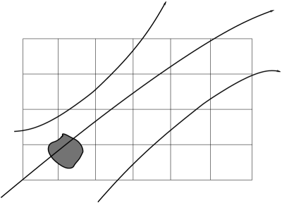
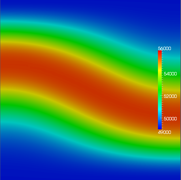
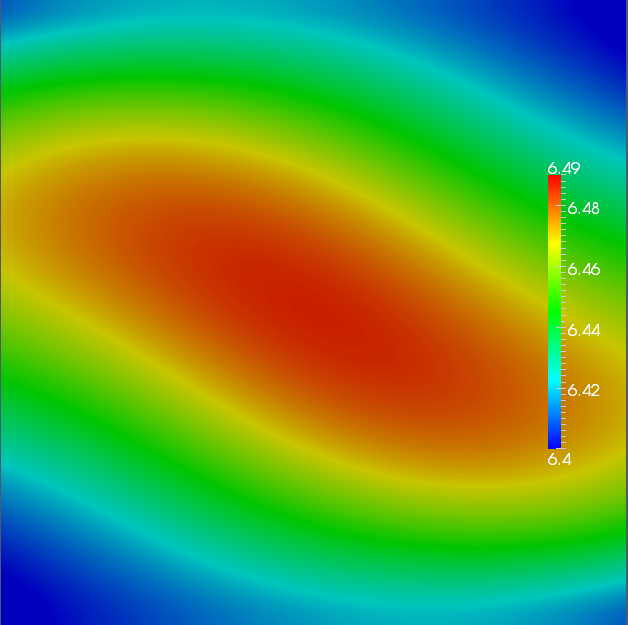
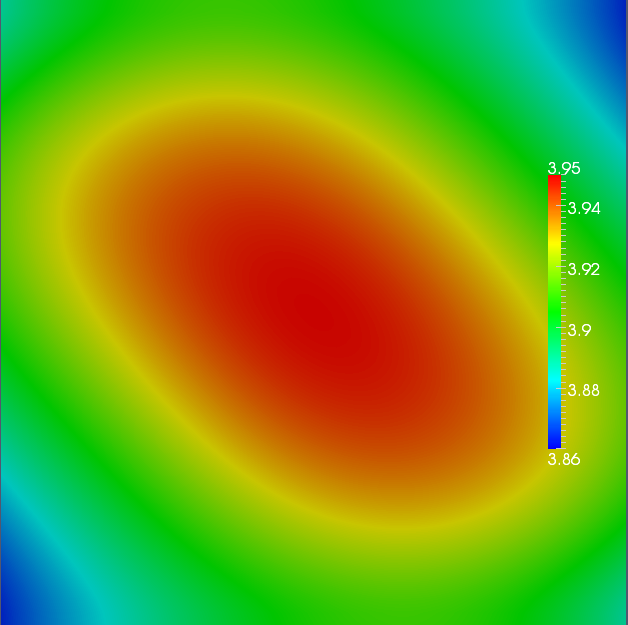
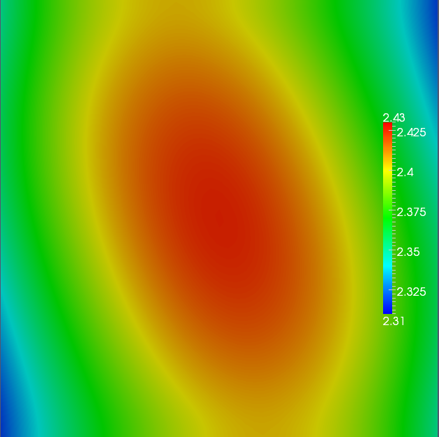
The aim of this paper will be to introduce an efficient numerical method, permitting to solve (2.3) accurately on a coarse Cartesian grid, which has not to be adapted to the field lines of and whose mesh size is independent of the value of . The here proposed scheme belongs to the category of Asymptotic-Preserving schemes, meaning they are stable independently of the small parameter and consistent with the limit problem, if tends to zero. The construction of the here developed AP-scheme is an adaptation of a method introduced by the authors in an elliptic framework (see [7]), to the here considered non-linear and time-dependent problem, and is based on a reformulation of the singularly perturbed problem (2.3) into an equivalent problem, which appears to be well-posed in the limit . But before introducing the AP-approach, we will start by studying in the following section the mathematical properties of problem (2.3). The test configuration chosen all along this paper is the diffusion of an initial temperature hot spot (see Figure 1) along arbitrary magnetic field lines .
2.1. Mathematical properties
Before starting with the presentation of the AP numerical scheme, let us first check some properties of the diffusion problem (2.3) for fixed . For notational simplicity, we consider a slightly more general form of problem (P)
| (2.7) |
for any . We obtain the particular case (2.3) by setting and redefining as for any . Equations of the type (2.7) are rather well studied in the literature. We refer to the classical works [8, 9, 13] as well as to the more modern literature on “The porous medium equation” as reviewed in [1, 22]. However, all these references normally treat only an isotropic version of the problem above, i.e. the non-linearity of the type is present in front of all the derivatives of . An anisotropic equation of the form (2.7) is studied in [11], but only in the case , so that the value of pertinent to our application is not covered. Another feature of our setting, which is not sufficiently covered in the existing literature, is the prescription of Robin boundary conditions. This is the reason why we wish to study in this paper the existence, uniqueness and positivity of solutions to (2.7).
We shall first introduce the concept of weak solution of problem (2.7) and state the existence/uniqueness theorem. Note that unlike the literature cited above, we assume from the beginning that the initial conditions are bounded and strictly positive, and prove the same properties for the weak solutions. Our treatment is thus performed under much less general assumptions than usually required, but this is quite enough for our application.
Definition 2.1.
(Weak solution) Let . Then with
is called a weak solution of problem (2.7), if and if for all one has
| (2.8) | |||
where .
Remark 2.2.
All the terms in this variational formulation are well-defined for any and . Indeed, as , and , one also has , and thus . This means that has a trace on , belonging to . As for all ( is bounded), one has , justifying thus the boundary integral in (2.8). Moreover, we have the continuous inclusion . This shows that one can impose the initial condition with .
Remark 2.3.
Actually, we have a sharper characterization of continuity in time for functions in . Indeed, let be a Banach space and let us denote by the space of weakly continuous functions with values in , which means for each the mapping is continuous. Then, one can prove (see [14] for more details) that .
Theorem 2.4.
Before proving this theorem, let us also define the sub- and super-solutions to problem (2.7) and establish a comparison principle for them.
Definition 2.5.
Lemma 1.
Proof.
For any , introduce the function as
and put . Note that since and thus . Observe also that the gradient of is zero outside from the set . Choosing this as the test function in the inequalities (2.8) for and and subtracting the second one form the first one gives
| (2.9) | |||
since and are of the same sign. We have moreover
on with a constant depending only on . Indeed, the first inequlity here holds for any and the second inequality follows by noting that on and on . We see that (2.9) combined with the inequality above implies
Let us now take the limit in this inequality. We have so that
| (2.10) |
On the other hand,
| (2.11) |
where denotes the positive part of . Indeed, a.a. on where denotes the Heaviside function ( for and for ). Observing that in the sense of distributions, proves (2.11) for sufficiently smooth . A standard density argument shows then that (2.11) actually holds for any . Note, in particular, that the terms at the right-hand side of (2.11) are well defined for functions in thanks to the inclusion , cf. Remark 2.3. Comparing (2.10) and (2.11) and taking into account on at , yields
| (2.12) |
which implies on . ∎
The construction of the following remarkable sub-solution is essentially due to M. Pierre [19].
Lemma 2.
Proof.
We will construct a smooth sub-solution satisfying all the announced properties. We thus rewrite the definition of a sub-solution in the strong form supposing from the beginning that :
| (2.13) | |||||
| (2.14) | |||||
| (2.15) |
The construction of such a function will be performed separately for the two cases mentioned in Hypothesis 1.
Case A: One can construct in this case a new coordinate system on such that the coordinate lines coincide with the -field lines and the surfaces are perpendicular to these lines. Domain is represented in these coordinates by a cylinder with and . We thus have with some scalar strictly positive field . We assume that the component of the boundary is represented by , is represented by and is represented by .
We are searching now for a sub-solution under the form where and are two positive decreasing functions which are yet to be adjusted. We observe immediately that on for all time so that (2.15) is automatically satisfied. The remaining boundary conditions (2.14) should be checked on and . We remind that on (). Similarly, on (). Substituting the Ansatz for into (2.14) now gives
This holds if one takes where .
It remains to check (2.13). Substituting the Ansatz for , this inequality is reduced to
| (2.16) |
Note that we have denoted the time derivative here by a dot and we neglected a term with since it is negative (the function is decreasing). We divide now both sides by and bound each term on the left-hand side as
and
We see now that inequality (2.16) will be satisfied if we require
| (2.17) |
with
One can thus take with any .
In summary, is a sub-solution. Clearly, for any one can take small enough so that . Moreover, for any , so that we have proved the statement of the Lemma putting , .
Case B: Let be a strictly positive function such that on , on and on with some sufficiently big constant , to be prescribed later.
We are searching now for a sub-solution under the form where are some positive constants which are yet to be adjusted. We observe immediately that (2.15) is automatically satisfied for such . The left-hand side of (2.14) can be written as
and thus it is negative provided is chosen sufficiently big. Indeed, is uniformly bounded from below by a positive constant in view of the geometrical hypothesis of case B.
It remains to check (2.13). Substituting the Ansatz for into this inequality yields
| (2.18) |
This inequality is satisfied provided we take and
Finally, for any one can take small enough so that . Lemma is thus proved also in case B.
∎
Remark 2.6.
In the case of a simple “aligned” geometry, i.e. and with a domain in , and supposing , one can easily construct a sub-solution satisfying a sharper estimate: under the assumptions of the preceding Lemma, there is a sub-solution such that
Indeed, one can repeat the proof as in case A of the preceding Lemma, taking , , up to the differential inequality (2.17). One observes now that so that one can take with any and . Our sub-solution is thus and as stated.
Let us now turn to the proof of our main result.
Proof of Theorem 2.4.
We shall first regularize the problem, in order to avoid the degeneracy. Then, in a second step, we shall treat the non-linearity via a fixed point argument. Finally, a priori estimates shall help us to pass to the limit in the regularized problem, to prove existence. The comparison principle above will be used to establish the uniqueness and the positivity of the solution. Let us now detail these steps.
1st step: Regularization
Fix and assume that is an upper bound for .
Introduce for notational simplicity the following functions
and consider the regularized version of (2.8): find (i.e. and such that and
| (2.19) |
By standard arguments, this problem is well posed. Indeed, consider the mapping
where we associate to any the unique solution of the linearized, regular parabolic problem
Indeed, taking , the mapping is well-defined, continuous and is relatively compact in . The continuity follows from the fact that for in and in , the Lebesgue dominated convergence theorem permits us to pass to the limit in the linearized term of the variational formulation. By Schauder fixed point theorem, has a fixed point , which provides a solution to (LABEL:var).
The solution of problem (LABEL:var) satisfies , provided we have . Indeed, define . Then one gets for the initial condition . Taking as the test function in the variational formulation (LABEL:var), yields immediately
which shows that . Since the same argument can be applied to any final time , we have in .
To prove the estimate from above, define . Observe that and take as the test function in the variational formulation (LABEL:var):
which shows that . Since again the same argument can be applied to any final time, we have in
2nd step: A priori estimates
In order to pass to the limit , we will need some a
priori estimates for the solution , independent of .
Taking in the variational formulation (LABEL:var) yields
which implies
| (2.20) |
with some constant .
Taking now in (LABEL:var), which is permitted since , yields
The first term can be rewritten as
with . Due to the facts that , and , we get
Thus, we have that the family , is bounded in . Moreover, is also bounded in , since and is uniformly bounded by some positive constant. Hence, is bounded in .
Let be the Banach space with the norm . For any in ,
with a constant independent of . This follows from the variational formulation (LABEL:var) with replaced by and from the estimates (2.20). We see thus that the family is bounded in . We remind also that is bounded in . Aubin-Simon compactness lemma [20] applied to the triple of spaces allows us now to conclude that the set is relatively compact in .
3rd step: Passage to the limit
The aim now is to pass to the limit in the
variational formulation (LABEL:var) in order to show the existence of a weak
solution of problem (2.3). The a priori estimates of the last step
permit us to show, that there exists a function satisfying in and such that after extracting a sub-sequence from , we have
To pass to the limit in the non-linear term, we use first the fact that is bounded in , so that there exists some function satisfying
In order to identify the function , we need some pointwise convergence of the sequence . For this, recall that the sequence is relatively compact in . Thus, up to a sub-sequence
Since for any fixed , , we have a.e. in . This permits to identify the function with , so that .
All these convergences allow now to pass to the limit in the variational formulation (LABEL:var) and to conclude the proof of existence for problem (2.7).
4th step: Positivity and uniqueness
Let be a weak solution to (2.7).
We use first the sub-solution constructed in Lemma 2 and the comparison principle in Lemma 1 to verify that with some positive constants small enough and large enough. We remark then that is a super-solution to (2.7). Again, by Lemma 1 we see that .
Let us remark here, that due to the strict positivity of the solution, in particular to the property that a.e. on , with some and , we have
3. Numerical method
3.1. Semi-discretization in space
The singular perturbation problem (2.3) is a highly anisotropic equation. Its variational formulation reads: find such that
for almost every . As mentioned already in Section 2, this problem becomes ill-posed if we take formally the limit . Indeed, only the leading term survives in this limit, so that any function from the space
would be a solution. It is easy to establish, however, the well-posed problem for the limit of the solutions to (P) as . Indeed, one can restrain the test functions in (P) to be in the space so that the -dependent term disappears and the correct problem in the limit reads: find such that
for almost every .
The discussion above shows that a straight-forward discretization of problem (P) may lead to very inaccurate results when . Indeed, setting would result in a singular problem, so that the problem with would be very ill-conditioned. To cope with this difficulty and to obtain a numerical scheme which is uniformly accurate with respect to , we introduce an Asymptotic-Preserving reformulation, very similar to the one introduced in [7]. The idea is to rewrite the singularly perturbed problem (3.1) in an equivalent form, which is however well-posed when one sets there formally and gives moreover the correct limit problem (L). In order to do this, we introduce the auxiliary unknown by the relation in and on , which rescales the nasty part of the equation permitting to get rid of the terms of order . The reformulated problem, called in the sequel the Asymptotic-Preserving reformulation (AP-problem) reads: find , solution of
| (3.22) |
where
| (3.23) |
System (3.22) is an equivalent reformulation (for fixed ) of the original P-problem (3.1). Putting now formally in (AP) leads to the well-posed limit problem
| (3.24) |
which is equivalent to problem (L). Note that acts here as a Lagrange multiplier for the constraint , which provides the uniqueness of the solution. Hence the AP-reformulation permits a continuous transition from the -model to the -model, which enables the uniform accuracy of the scheme with respect to .
Let us now choose a triangulation of the domain with triangles or quadrangles of order and introduce the finite element spaces and of type or on this mesh. The finite element discretization of (3.22) writes then: find such that
| (3.25) |
Remark that this system is continuous in time and also nonlinear, such that one has to develop now a procedure for the linearization and the discretization in time. This procedure has to be chosen carefully, such that the AP-property developed so far, is not destroyed. This is the aim of the next section.
3.2. Semi-discretization in time
In order to approach numerically the time derivative in (3.25), we introduce three different schemes : a standard first order, implicit Euler scheme, the Crank-Nicolson scheme and a second order, L-stable Runge-Kutta method. We show in the following that the first order Euler-scheme is stable and asymptotic-preserving. The Crank-Nicolson schemes gives reliable results and second order convergence under certain assumptions, but is not asymptotic-preserving. Thus, if second order accuracy in time is desired, the L-stable Runge-Kutta method has to be applied. All three methods are exposed to numerical tests and compared in Section 4.
3.2.1. Implicit Euler scheme
Introducing the forms
| (3.26) | |||
| (3.27) | |||
| (3.28) |
allows us to write the first order, implicit Euler method in the compact notation: Find , solution of
| (3.31) |
where the non linear term was replaced by a first order approximation in :
| (3.32) |
A slightly different first order AP-scheme was introduced in [16] for the resolution of the same temperature balance problem. There, the (P)-problem was firstly discretized in time (implicit Euler), then linearized by a fixed point mapping, and finally the AP reformulation applied. The numerical results obtained in [16] are similar to the present ones.
3.2.2. Linearized Crank-Nicolson scheme
To construct a scheme, which is second order in time, one can come to the idea to employ the Crank-Nicolson scheme: Find , solution of
| (3.35) |
As one can observe, we have to deal for each fixed , with a nonlinear equation. In the linear terms, one can set . To linearize the term however, we shall use the standard linear extrapolation method. In other words, the non-linearity in this last formula, , will be replaced by a linearized second order approximation in :
| (3.36) |
The resulting linear system reads finally: Find , solution of
| (3.41) |
Unfortunately, this method is not Asymptotic-Preserving. For small values of one expects that the solution will immediately fall into the space of functions almost constant in the direction of the anisotropy, no matter what initial condition was imposed. In the case of the Crank-Nicolson scheme for large time steps compared to , the second equation in (3.41) will constrain the numerical solution to oscillate if the initial condition is not already in the suitable space. This requires the restrictive choice of a time step of the order of , which yields the method inapplicable in general cases. In other words, the Crank-Nicolson scheme is unable to model diffusion processes for large , due to the inadequate approximation of the damping processes. The Crank-Nicolson scheme is A-stable but not L-stable and the AP-property of a scheme is strongly related to the L-stability of the scheme.
As an example of the non-convergence of the () scheme in a general case, we show some numerical results corresponding to a test case defined in the Section 4.2.2. The initial condition is a Gaussian peak located in the center of the computational domain with a maximum of . If the time step is too large, than will immediately reach negative values and thus the numerical algorithm will fail in the next iteration. However, if is sufficiently small the () scheme is of second order in time. Unfortunately, the biggest time step that does not provoke oscillations in the numerical solution, is of the order of , for an initial Gaussian peak of . This makes the () scheme of no practical use in real simulations. These results are plotted on Figure 2.
3.2.3. L-stable Runge-Kutta method
As we are interested in an AP-scheme, which is second order accurate in time, we propose now a two stage Diagonally Implicit Runge-Kutta (DIRK) second order scheme, which does not suffer from the limitations of the Crank-Nicolson discretization. The scheme is developed according to the following Butcher’s diagram:
| (3.45) |
with .
Remark 3.1.
(Butcher’s diagram) The coefficients of the -stage Runge-Kutta method are usually displayed in a Butcher’s diagram :
| (3.50) |
Applying this method to approximate to following problem
| (3.51) |
reads: For given , being an approximation of , the is determined accordingly to :
| (3.52) | |||
| (3.53) |
If for than .
The scheme (3.45) is known to be L-stable, thus providing the Asymptotic Preserving property. The scheme writes: Find , solution of
| (3.65) |
with (respectively ) being the solution of the first (respectively second) stage of the Runge-Kutta method. The terms and are respectively the second order time-approximations of and , used to linearize the problem.
For each time step we have therefore to assemble and solve two linearized problems. This method is two times slower than the Crank-Nicolson scheme, with the advantage however of maintaining the AP-property of the scheme, advantage which is crucial for .
4. Numerical results
In this section we compare the proposed implicit Euler-AP and DIRK-AP schemes with a standard linearized implicit Euler discretization of the initial singular perturbation problem (2.3), given by
| (4.66) |
4.1. Discretization
Let us present the space discretization in a 2D case. We consider a square computational domain . All simulations are performed on structured meshes. Let us introduce the Cartesian, homogeneous grid
| (4.67) |
where and are positive even constants, corresponding to the number of discretization intervals in the - resp. -direction. The corresponding mesh-sizes are denoted by resp. . Choosing a finite element method (-FEM), based on the following quadratic base functions
| (4.74) |
for even and
| (4.79) |
for odd , we define the space
The spaces and are then defined by
The matrix elements are computed using the 2D Gauss quadrature formula, with 3 points in the and direction:
| (4.80) |
where , , and , which is exact for polynomials of degree 5. Linear systems obtained for all methods in these numerical experiments are solved using a LU decomposition, implemented by the MUMPS library.
4.2. Numerical tests
4.2.1. Known analytical solution
First, let us construct a numerical test case with a known solution. Finding an analytical solution for an arbitrary -field presents a considerable difficulty. In the previous paper [6], we presented a way to find such a solution. Let us recall briefly how to do this. The starting point is a limit solution
| (4.81) |
where is a numerical constant aimed to control the variations of . For , the limit solution represents a solution for the constant case. The parameter is the scaling of .
Since is a limit solution, it is constant along the field lines. Therefore we can determine the field using the following implication
| (4.82) |
which yields for example
| (4.85) |
Note that the field , constructed in this way, satisfies , which is an important property in the framework of plasma simulations. Furthermore, we have in the computational domain. Now, we choose to be a function that converges, as , to the limit solution , for example
| (4.86) | |||
| (4.87) | |||
| (4.88) |
In our simulations we set so that the direction of the anisotropy is variable in the computational domain. Note that we have
| (4.89) | |||
| (4.90) |
The problem is supplied with a force term computed accordingly.
As an initial condition we take , with defined by (4.88). In this setting we expect both Asymptotic-Preserving methods () and () to converge in the optimal rate, independently on and .
First we test the space convergence of the methods. To do this we choose a small time step such that the time discretization error is much smaller than the space discretization error. We then vary the mesh size and perform simulations for 100 time steps. The results are summarized in Table 1 and Figure 3. All three methods give as expected the third order space convergence in the -norm for large values of . Moreover, due to the extremely small time step, the numerical precision is the same, even if one uses second or first order methods. For small values of only the Asymptotic Preserving schemes give good numerical solutions.
| -error | |||
|---|---|---|---|
| P | |||
| 0.1 | |||
| 0.05 | |||
| 0.025 | |||
| 0.0125 | |||
| 0.00625 | |||
| -error | |||
|---|---|---|---|
| P | |||
| 0.1 | |||
| 0.05 | |||
| 0.025 | |||
| 0.0125 | |||
| 0.00625 | |||
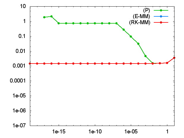
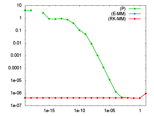
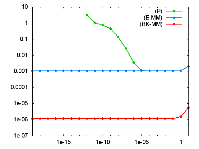
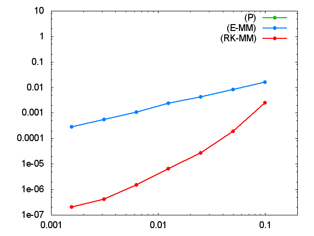
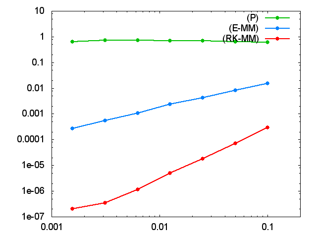
Finally we test the time convergence of the methods. To do this we choose a small mesh size such that the space discretization error is smaller than the time discretization error. We then vary the time step and perform simulations on a fixed grid. The results are summarized in Table 2 and Figures 4 and 5. Note that the scheme is of second order in time as long as the error due to the time discretization dominates the error induced by the space discretization. The standard (P)-scheme works well and is of first order, as long as is close to one. The scheme is of first order for all values of the anisotropic parameter. Also note that while the scheme demands twice more computational time than the scheme, it gives much better precision. In order to achieve a relative error of the order of for it suffices to take a time step of in the RK-scheme. A comparable accuracy with is obtained for a time step 16 times smaller. In the case of the ratio is 32.
| -error | |||
|---|---|---|---|
| P | |||
| 0.1 | |||
| 0.05 | |||
| 0.025 | |||
| 0.0125 | |||
| 0.00625 | |||
| 0.003125 | |||
| 0.0015625 | |||
| -error | |||
|---|---|---|---|
| P | |||
| 0.1 | |||
| 0.05 | |||
| 0.025 | |||
| 0.0125 | |||
| 0.00625 | |||
| 0.003125 | |||
| 0.0015625 | |||
To conclude, one can remark that the asymptotic-preserving schemes, () and (), are uniformly accurate with respect to the perturbation parameter . This essential feature can be very useful in situations where the anisotropy is variable in space, i.e. the parameter is -dependent. No mesh-adaptation is any more needed in these cases, a simple Cartesian grid enables accurate results, with no regard to the -values.
4.2.2. Initial Gaussian peak
The second investigated test is the evolution of the following initial Gaussian peak, located in the middle of the computational domain:
| (4.91) |
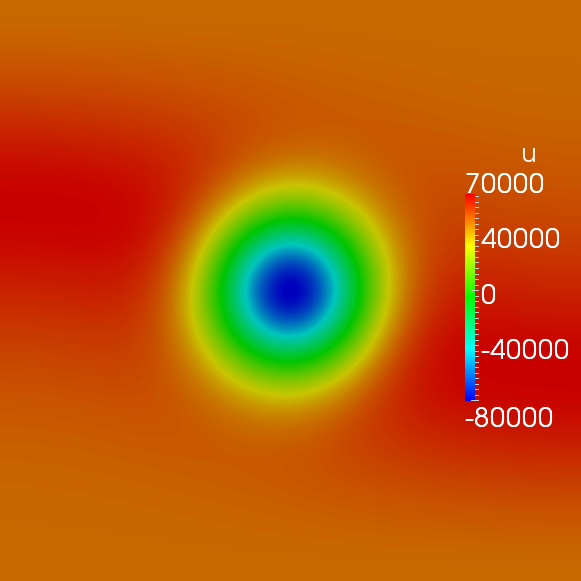
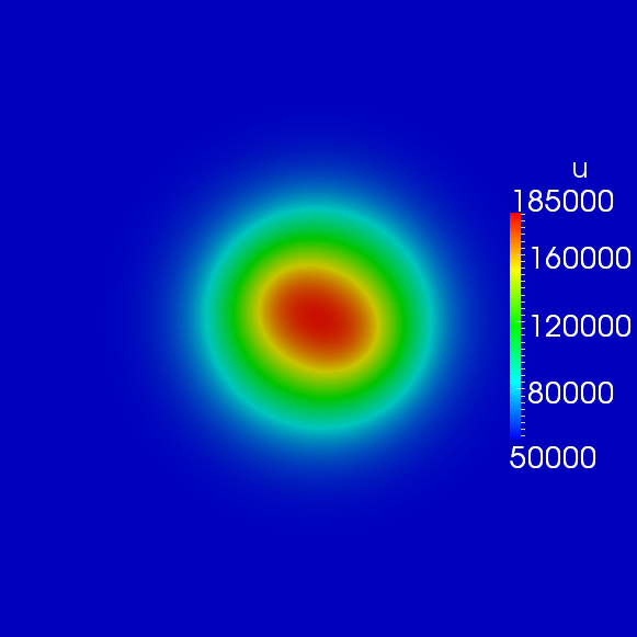
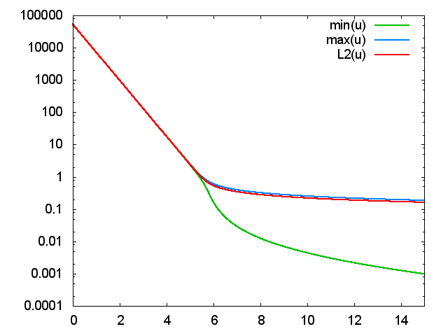
where is the maximal temperature in the domain and the anisotropy direction is given as in the previous tests. We perform numerical experiments with the choice of . We choose the time step and perform numerical simulations on a fixed grid with the final time set to . The time step is big compared to the time scale induced by the initial condition. Indeed, after the first iteration of the algorithm the numerical solution immediately falls into the space of functions which are almost constant in the direction of the anisotropy (see Figure 7). The evolution of the numerical solution consists of two phases. The first one, in which the parallel components of the diffusion operator dominate, is characterized by the exponential decay of , and (see Figure 6). When reaches some critical value, the parallel part of the diffusion operator becomes smaller than the perpendicular one. The direction of the strong diffusion is now inverted and the numerical solution aligns itself rather with the perpendicular direction. The minimum, maximum as well as the -norm of continue to approach zero, but the decay is no longer exponential. The -norm and the maximal value remain close to each other and almost constant in time. The minimal value of , as well as the boundary-values decrease much faster.
5. Conclusion
The here presented Asymptotic-Preserving scheme proves to be an efficient, general and easy to implement numerical method for solving nonlinear, strongly anisotropic parabolic problems. This kind of problems occur in several important applications, as for example magnetically confined fusion plasmas. The method is based on a reformulation of the problem, initially introduced by the authors in an elliptic framework, and a careful linearization as well as time-discretization of the resulting equation, which does not destroy the AP-properties of the space-discretization. Numerical experiments show clearly the advantages of such an AP-scheme.
Acknowledgments
The authors would like to thank Michel Pierre and Giacomo Dimarco for useful discussions. This work has been partially supported by the ANR project ESPOIR (Edge Simulation of the Physics Of Iter Relevant turbulent transport, 2009-2013) and the ANR project BOOST (Building the future Of numerical methOdS for iTer, 2010-2014).

References
- [1] D. Aronson. The porous medium equation. A. Fasano, M. Primicerio (Eds.), Nonlinear Diffusion Problems, Lecture Notes in Mathematics, 1224:1 –46, 1986.
- [2] S. F. Ashby, W. J. Bosl, R. D. Falgout, S. G. Smith, A. F. Tompson, and T. J. Williams. A Numerical Simulation of Groundwater Flow and Contaminant Transport on the CRAY T3D and C90 Supercomputers. International Journal of High Performance Computing Applications, 13(1):80–93, 1999.
- [3] P. Basser and D. Jones. Diffusion-tensor mri: theory, experimental design and data analysis–a technical review. NMR in Biomedicine, 15(7-8):456–467, 2002.
- [4] C. Beaulieu. The basis of anisotropic water diffusion in the nervous system–a technical review. NMR in Biomedicine, 15(7-8):435–455, 2002.
- [5] B. Berkowitz. Characterizing flow and transport in fractured geological media: A review. Advances in Water Resources, 25(8-12):861–884, 2002.
- [6] P. Degond, F. Deluzet, A. Lozinski, J. Narski, and C. Negulescu. Duality-based asymptotic-preserving method for highly anisotropic diffusion equations. arXiv:1008.3405v1, 2010.
- [7] P. Degond, A. Lozinski, J. Narski, and C. Negulescu. An asymptotic-preserving method for highly anisotropic elliptic equations based on a micro-macro decomposition. arXiv:1102.0904v1, 2012.
- [8] Y. Dubinskii. Some integral inequalities and the solvability of degenerate quasi-linear elliptic systems of differential equations. Matematicheskii Sbornik, 106(3):458–480, 1964.
- [9] Y. Dubinskii. Weak convergence for nonlinear elliptic and parabolic equations. Matematicheskii Sbornik, 109(4):609–642, 1965.
- [10] S. Günter, K. Lackner, and C. Tichmann. Finite element and higher order difference formulations for modelling heat transport in magnetised plasmas. Journal of Computational Physics, 226(2):2306–2316, 2007.
- [11] H. Jian and B. Song. Solutions of the anisotropic porous medium equation in under an -initial value. Nonlinear analysis, 64(9):2098–2111, 2006.
- [12] S. Jin. Efficient asymptotic-preserving (AP) schemes for some multiscale kinetic equations. SIAM J. Sci. Comput., 21(2):441–454, 1999.
- [13] J. Lions. Quelques méthodes de résolution des problèmes aux limites non linéaires. Gauthier-Villars, 1969.
- [14] J.-L. Lions and E. Magenes. Non-homogeneous boundary value problems and applications. Vol. I. Springer-Verlag, New York, 1972. Translated from the French by P. Kenneth, Die Grundlehren der mathematischen Wissenschaften, Band 181.
- [15] H. Lutjens and J. Luciani. The xtor code for nonlinear 3d simulations of mhd instabilities in tokamak plasmas. Journal of Computational Physics, 227(14):6944–6966, 2008.
- [16] A. Mentrelli and C. Negulescu. Asymptotic preserving scheme for highly anisotropic, nonlinear diffusion equations. application: Sol plasmas. submitted to JCP, 2012.
- [17] W. Park, E. Belova, G. Fu, X. Tang, H. Strauss, and L. Sugiyama. Plasma simulation studies using multilevel physics models. Physics of Plasmas, 6:1796, 1999.
- [18] P. Perona and J. Malik. Scale-space and edge detection using anisotropic diffusion. Pattern Analysis and Machine Intelligence, IEEE Transactions on, 12(7):629–639, 1990.
- [19] M. Pierre. Personal communication, 2011.
- [20] J. Simon. Compact sets in the space . Ann. Mat. Pura Appl. (4), 146:65–96, 1987.
- [21] P. Tamain. Etude des flux de matière dans le plasma de bord des tokamaks. PhD thesis, Marseille 1: 2007., 2007.
- [22] J. Vázquez. The porous medium equation: mathematical theory. Oxford University Press, USA, 2007.
- [23] J. Weickert. Anisotropic diffusion in image processing. European Consortium for Mathematics in Industry. B. G. Teubner, Stuttgart, 1998.
- [24] J. Wesson. Tokamaks. Oxford University Press, New York, NY, 1987.