Chameleon: A Reconstruction package for a KM3NeT detector

0.1 Introduction

In this note we describe the Chameleon software we developed for the event reconstruction of KM3 detector. This software package’s developement started as a standalone application before the endorcement from the KM3NeT consortium of the SeaTray software framework, but it was adapted to it on the course.

Chapter 1 outlines the techniques we developed for the pattern recognition and the track fitting. In Chapter 2, we demonstrate the performance of the Chameleon Reconstruction.

Chapter 1 Pattern Recognition and Fitting

There are two main parts in the reconstruction package: The patern recognition and the fitting. The first part is designed for a km³ multi PMT Optical Modules detector (see e.g. [2]). It consists of a algorithms for the selection and grouping of hits in track canidates.

The second is a generic $\chi^{2}$ minimizer. This is generic enough to allow for unbiased comparison between different detector designs.

Before the description of the the pattern recognition and fitting algorithms we give a short description of the specific data sets used for this report.

1.1 Data Sets

The demonstration of the reconstruction is done on a sample of 6,000,000 MC neutrinos produced through the de facto standard tools provided with the seatray, namely nugen for the production and g4sim for the simulation.

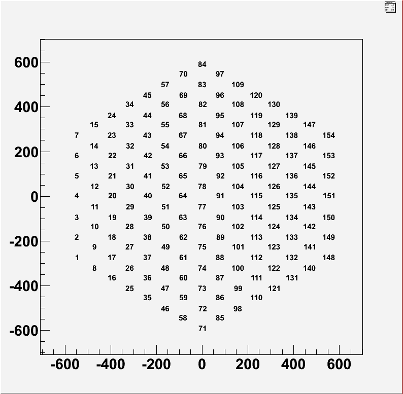
Figure 1.1: The detector geometry used in this study.

In this data set, no light scattering in water was simulated. ${}^{40}K$ noise was simulated at a rate of $8KHz$ per PMT, which is more than the commonly accepted rate for these tubes of $5.2KHz$, since more noise would be a stringent test of the filtering out of the noise. For a detailed description of the whole simulation, see [11].

The detector used is a small, dense detector of 154 strings (fig. 1.1), with string distance 92 m. Each string has an active length of 570 m., and 20 Multi PMT Optical Modules at 30 m. distance between each other. Each OM is equipped with 31 $3^{\prime\prime}$ PMTs.

The produced $\nu$-spectrum, which corresponds to an $E^{-1}$ flux, is presented in fig. 1.2, while the respective quantities for charged current produced muons in fig. 1.3.

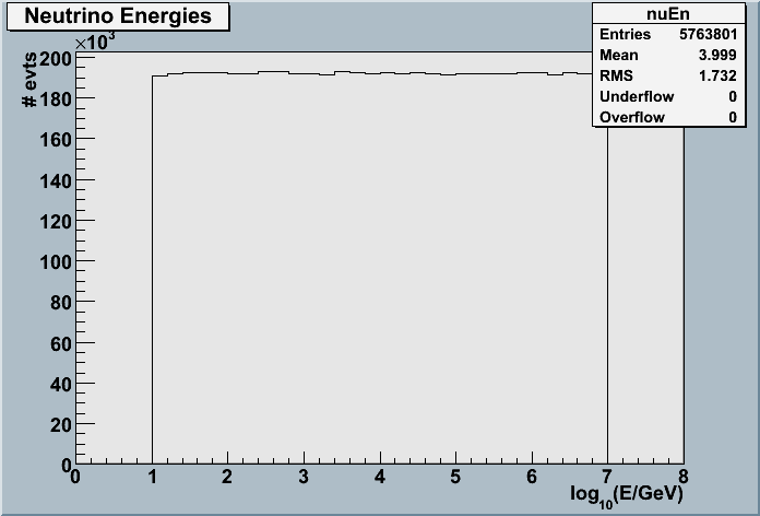
(a) Generated $\nu$ energies

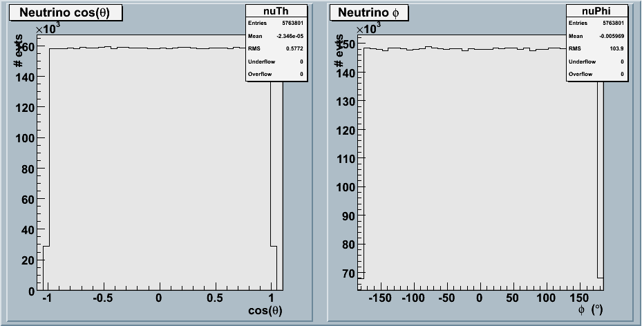
(b) $\theta$ and $\phi$ angle distribution

Figure 1.2: Generated $\nu$ spectra.

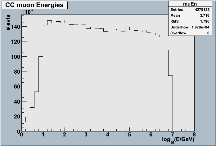
(a) Generated CC $\mu$ energies

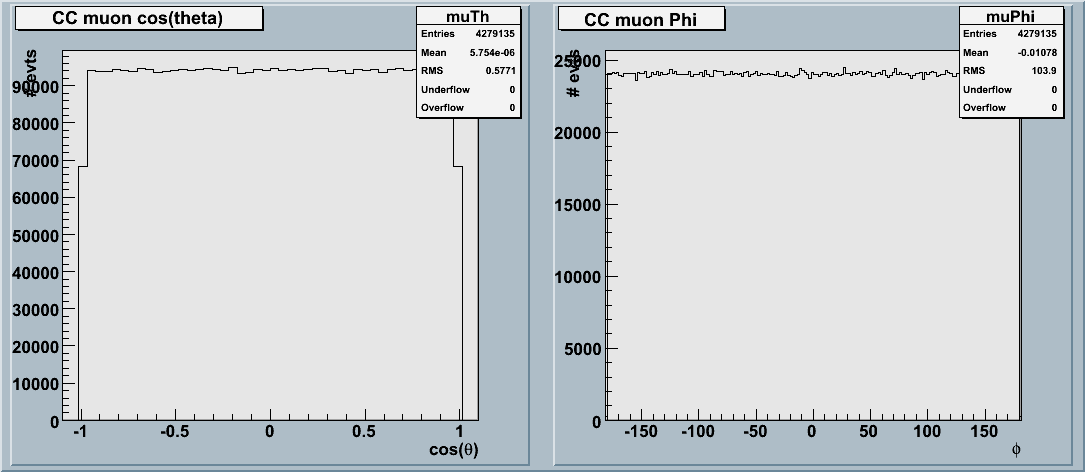
(b) $\theta$ and $\phi$ angle distribution

Figure 1.3: Generated CC $\mu$ spectra.

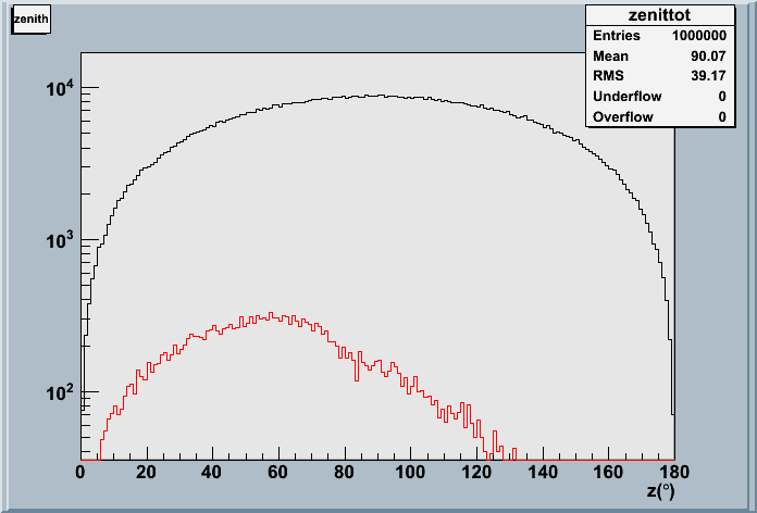
(a) Distribution of muons as a function of zenith  $z$

(b) Distribution of muons as a function of $\cos(z)$

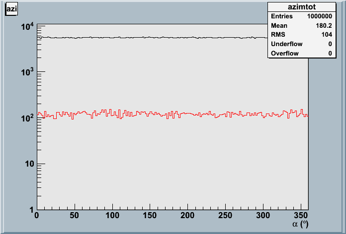
(c) Distribution of muons as a function of $\alpha$

Figure 1.4: Angle distributions for $\mu$’s.: Black all $\mu$’s, Red reconstructed $\mu$’s

A measure of the total number of produced photons is the number of OMs that fired, which is shown in fig. 1.5a, for CC events and in 1.5b for NC events. CC events are defined by the existence of a primary muon in the particle tree, while NC events by the absence thereof.

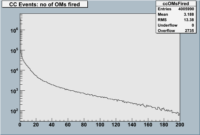
(a) CC events

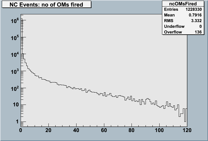
(b) NC events

Figure 1.5: Numbers of OMs fired.

The flat input neutrino spectrum is transformed into the relevant fluxes with the use of the “NeutrinoFlux” module (implemeneted originaly for IceCube). Specifically we use functions ConventionalNeutrinoFlux("bartol_numu") and
PromptNeutrinoFlux("naumov_rqpm_numu"). The first simulates the conventional muon flux (leptons from $\pi^{\pm}$’s and Kaons), while the second simulates leptons from charm decays. The atmospheric flux is the sum of these two functions.

1.2 Fitting

An integral part of the pattern recognition are the methods developped for the fitter, so a description of the fitting algorithm will necessarily precede the description of the hit selection and final reconstruction.

The fitter is an implementation of a $\chi^{2}\;$minimization with the help of the C++ Minuit2 package (embedded within ROOT). The minimization is done according to the geometrical model of fig. 1.6.

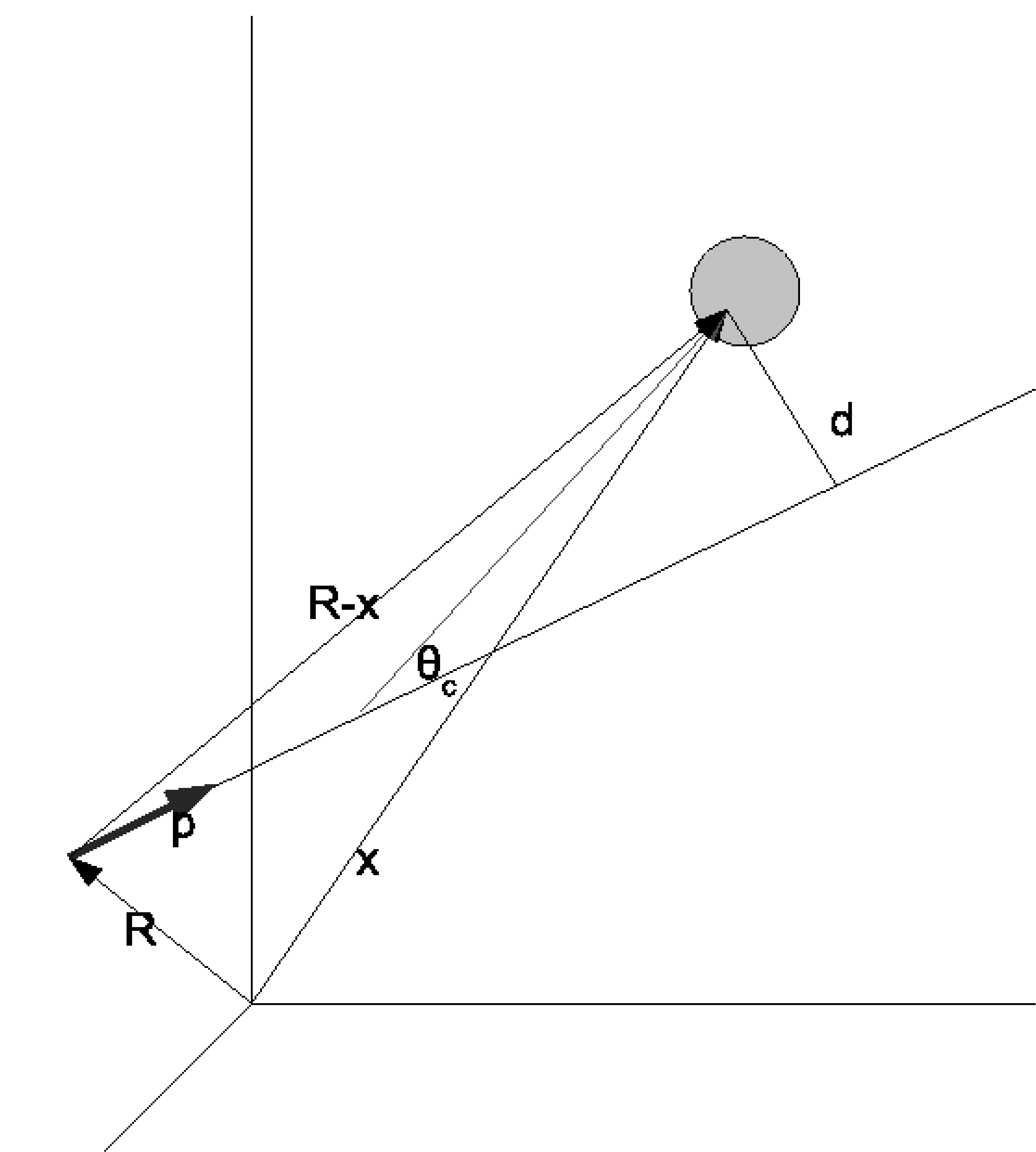
Figure 1.6: The geometrical model used for the minimization. The Čerenkov index used is for $\lambda=460nm$ ($43.5^{\rm o}$).

Specifically, if a muon with (pseudo) vertex at $\bf{R}$ and momentum direction $\bf{p}$, emits a photon that hit a PMT at $\bf{x}$, the total time between the vertex and the hit is given by

$$c\;t^{exp}=\sin\theta_{c}\sqrt{(\bf{x}-\bf{R})^{2}-\left[\bf{p}\cdot(\bf{x}-\bf{R})\right]^{2}}+\bf{p}\cdot(\bf{x}-\bf{R}),$$ (1.1)

where $\theta_{c}$ the Čerenkov angle. The $\chi^{2}\;$function that is minimized is

$$\chi^{2}=\sum_{i}\frac{t_{i}^{exp}-t_{i}^{data}}{\sigma_{i}},$$ (1.2)

where $t_{i}^{exp}$ is the expected arrival time of the $i$th photon of eq. (1.1), assuming that the measured pulse is the PMT response to Čerenkov light originating from a muon track, $t_{i}^{data}$ is the actual measured time, and $\sigma_{i}$ is the error ascossiated with the $i$th hit. This error is set equal to 2 ns.

Within the project, two distinct strategies for the estimation of track parameters were implemented. They are based on an assesment of the hit residuals wrt the track, as it is produced by the fit.

• Fit with Rejection: This is a recursive fit, which calculates the hit residuals and rejects those hits that are $N\sigma$ away from the nominal value of $2~{}ns$.

• Constant deweight: All hits are deweighted and their $\sigma$ is set equal to a constant parameter.

The fitter is able to calculate the track parameters in either cartesian coordinates (track vertex ${\bf R}(x,y,z)$ and zenith and azimuth angles) or in spherical coordinates (vertex ${\bf R}(r,\theta,\phi)~{})$ for a track candidate with at least 6 PMTs hit.

1.3 Pattern Recognition

1.3.1 ${}^{40}\!K$ filter and hit selection

One of the problems with a sea $\nu$-telescope is ${}^{40}K$ noise. The first part of chameleon needs to clean up as much noise as possible, since a $\chi^{2}\;$reconstruction is very sensitive to noise.

To use the potential of multi-PMT OMs, the algorithm uses a slightly modified wrt the proposed “write up string designs” [2] scheme.

The first modification is that for each PMT only the first photon is considered to be a hit, while the charge is set equal to the total number of photons this particular PMT registered (i.e. one has only one hit per PMT). This was deemed necessary until the final time over threshold mechanism in the MC is stabilized. The second modification is that not only adjacent PMTs are taken into account (see below).

The ${}^{40}\!K$ filter is based on a two-layered algorithm, the trigger algorithm and the hit selection.

The trigger algorithm is based roughly on the L1 trigger (see [2]), as broadened after a MC study of timings for photons. Specifically, for all the hits that are registered on an OM, the first thing to do is to select the data set that will be sent to the reconstruction. Since signal photons are concentrated around the track that created them while noise is randomly produced, a first filter can be based on time coincidences of hits. In fig.(1.7) the differences in time of arrival between succesive hits for OMs with 2 or more hits are plotted for noise production rate of 8 kHz per PMT. It should be noticed here that although the expected noise level for the Multi-PMT design is at 5.2 kHz per PMT, a higher level of noise was used for reasons, in order to be on the safe side. If both hits are photons, they are registered in blue. It can be seen clearly that when two succesive hits on the same OM are registered within 6 ns or less, then they are most probably both real photons.

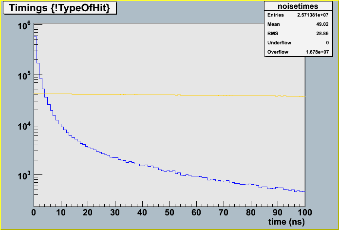
(a) Time differences between succesive hits per OM.

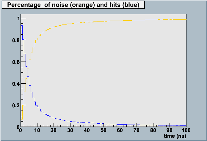
(b) Ratios of Čerenkov photons and noise photons wrt the total number, for the same sample.

 

Figure 1.7: Time differences between pairs of succesive hits per OM. Blue = both hits are photons, orange = at least one hit is noise.

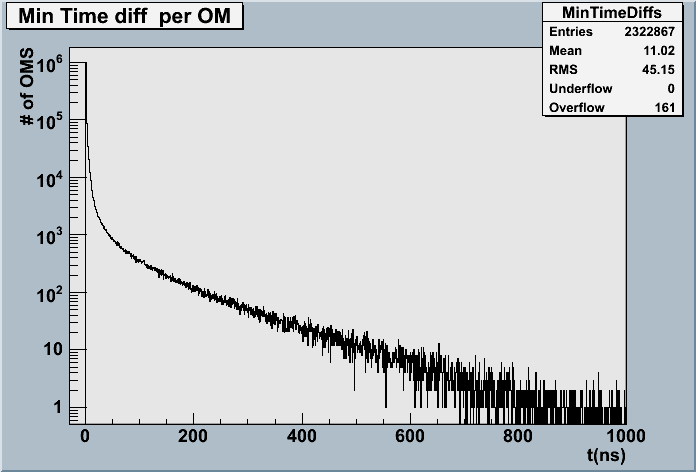
Figure 1.8: For each OM with more than one photon, choose the 2 photons which are closest in time and plot their time difference. One such pair per OM can be plotted.

(a) Time residual for hits with charge equal to 1.

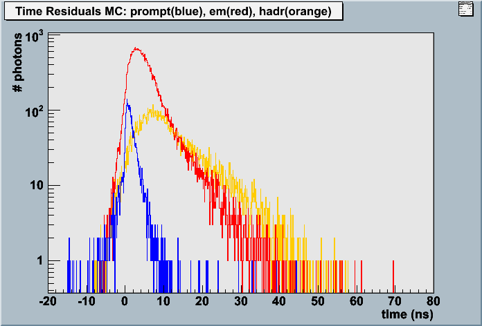
(b) Time residual for hits with charge equal to 3.

Figure 1.9: Time residuals.

The detailed description of these algorithms is as follows:

• Only use the first photon for each PMT within an event. This is done in order to keep the results totally unbiased as to the exact electronics of the system. After the finalization of the T/threshold mechanism, the information from the rest of the photons will be used.

• Start by looping over all the OMs of the event. At this layer consider only OMs with 2 or more detected hits.

  • After ordering the hits of each OM in time, find which two of them are closest. Check their time difference $\Delta t$: If the following condition does not hold

    $$|\Delta t|<6\;ns,$$ (1.3)

    the whole OM is discarded, as it is assumed that since the smallest time difference is larger than the OM’s diameter the photons are too sparse to be real photons, see e.g. [6, p.60] and fig. (1.7).

  • In case eq. (1.3) is satisfied, then perform a local loop over the photons of this particular OM, starting from the minimum time pair. Keep only those photons that are no further away than $7\;ns$ from the previous photon.

• After this first filtering, find those OMs that have registered the largest numbers of hits (number of PMTs times charge). Only keep the event if the “largest” OM has registered hits in at least 3 of its PMTs. These “large” OMs are subsequently grouped by causal connection. Each of these clusters of “large” OMs will be used as a basis for track reconstruction in the next steps, leading possibly to multiple tracks.

• Loop over these OM’s closest neighbours, i.e. those OMs that are located within 180 m ($\sim$ 3 absorbtion lengths) from the OM with the largest hit. The closest neighbors are OMs that did not pass the trigger, so by checking causal connections with the large OMs, more hits can be retrieved. For string distances larger than 180 m this means that this search is reduced to same-string OMs.

• Obviously, the number of active (i.e. that have at least one hit on one of their PMTs) neighbouring OMs is smaller than the number of neighbouring OMs. The photons on the closest neighbours’ PMTs are required to obey the condition

  $$-T_{0}<|\Delta t|-\frac{r}{c}<t_{0},$$ (1.4)

  where $r$ is the distance between OMs under consideration, $T_{0}$ and $t_{0}$ are arbitrary constants and the time difference $\Delta t$ is calculated between the current photon’s time and the time of the first photon of the “large” OM under consideration (For a justification see e.g. [7, fig 5.2].)

  In fig. 1.10, the quantity $|\Delta t|-\frac{r}{c}$ of eq. (1.4) is plotted for a data sample of a small detector with string distances at only 90m. As can be seen from the first of these figures, for a neighbourhood of $R=120$ m around the largest OM, one can take into account all the photons below $t_{0}$, since there the ${}^{40}\!K$s remain a small percentage of the total number of photons. Unfortunately, as the radius increases, the local time window, equal to the time it takes a muon to travel one such radius $\sim R/c$, is large enough for more ${}^{40}\!K$ photons to be considered: $R/c=400,600,667$ ns, for the 3 radii. In the following tests $T_{0}$ was set to 300 ns for $R=180$ and $200$, while it is not important for 120 m where the filter is more effective (in the latter case of course there are fewer photons so that the next step of reconstruction is harder).

  

  (a) Photons in a sphere of 120 m.

  

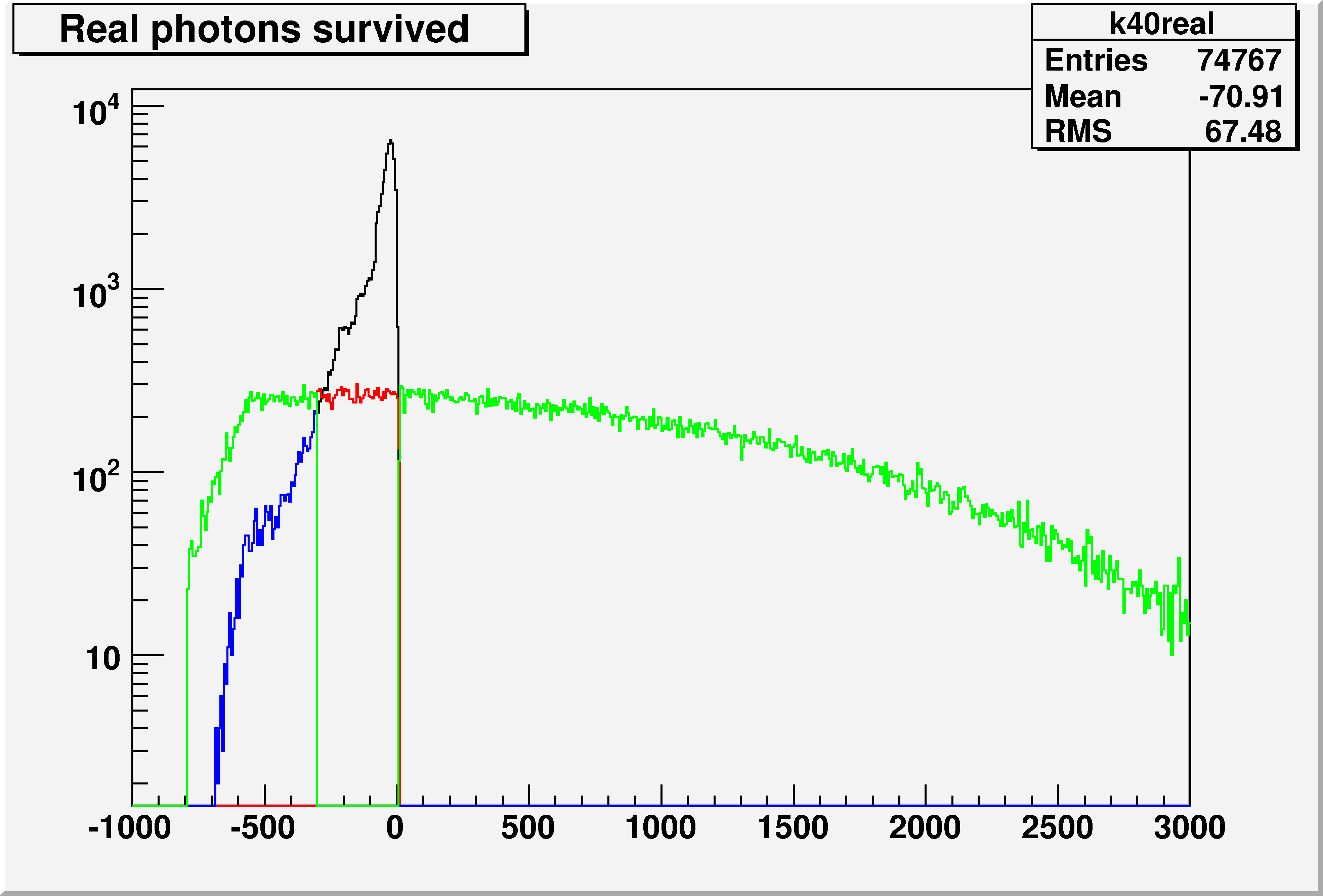
  (b) Photons in a sphere of 180 m.

  

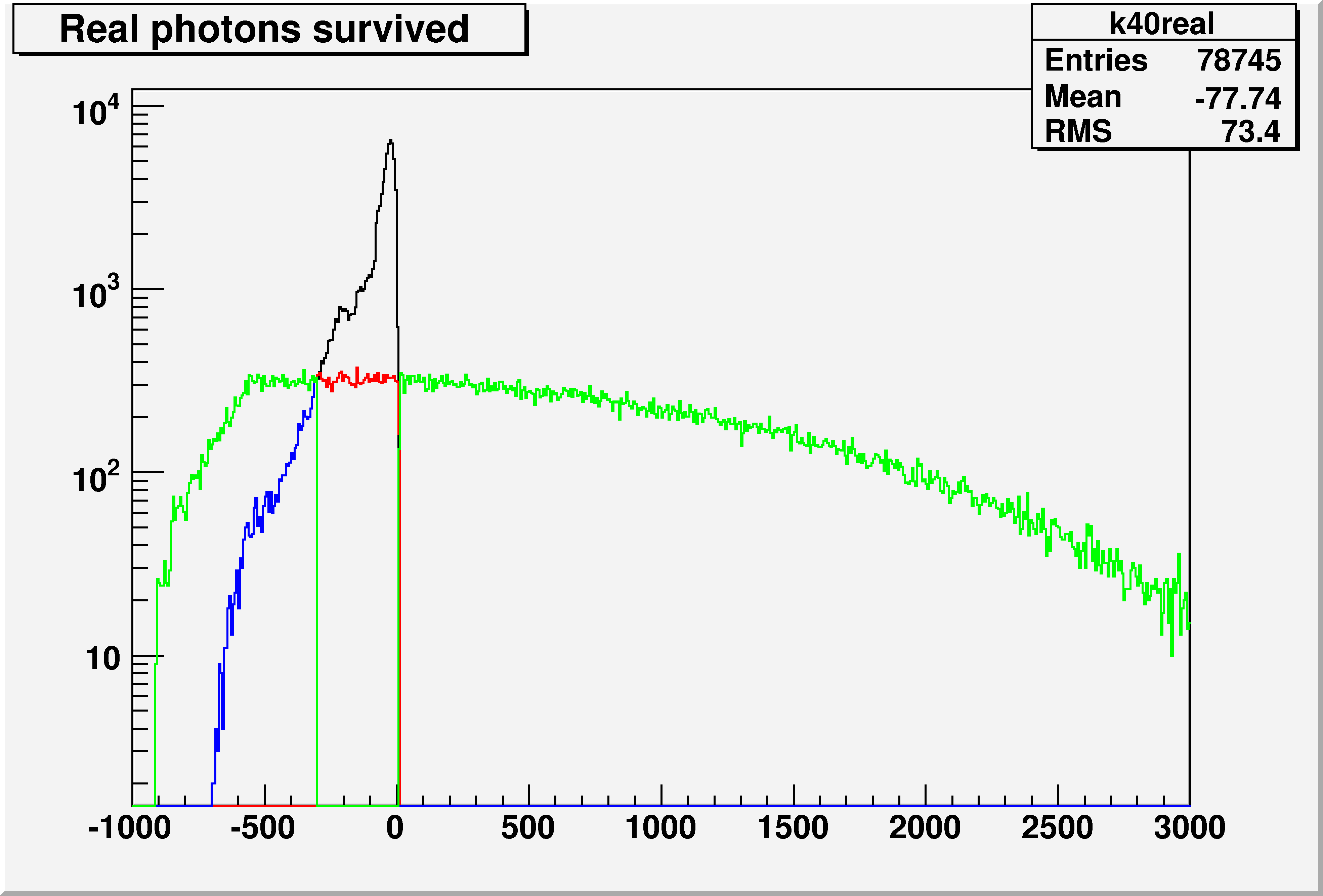
  (c) Photons in a sphere of 200 m.

  Figure 1.10: A plot of eq. (1.4). Only photons within a sphere of 120, 180 and 200 m respectively are taken into account. Black: survived real photons. Red: Survived ${}^{40}\!K$. Blue: Rejected real photons. Green: Rejected ${}^{40}\!K$.

  The combination of these 2 filters eliminates most of ${}^{40}\!K$ photons, as can be seen in fig. 1.11. A major problem whcih should be considered is the fact that as the number of OMs under consideration rises, so does the relative number of ${}^{40}\!K$ hits which survive the causality filter.

  

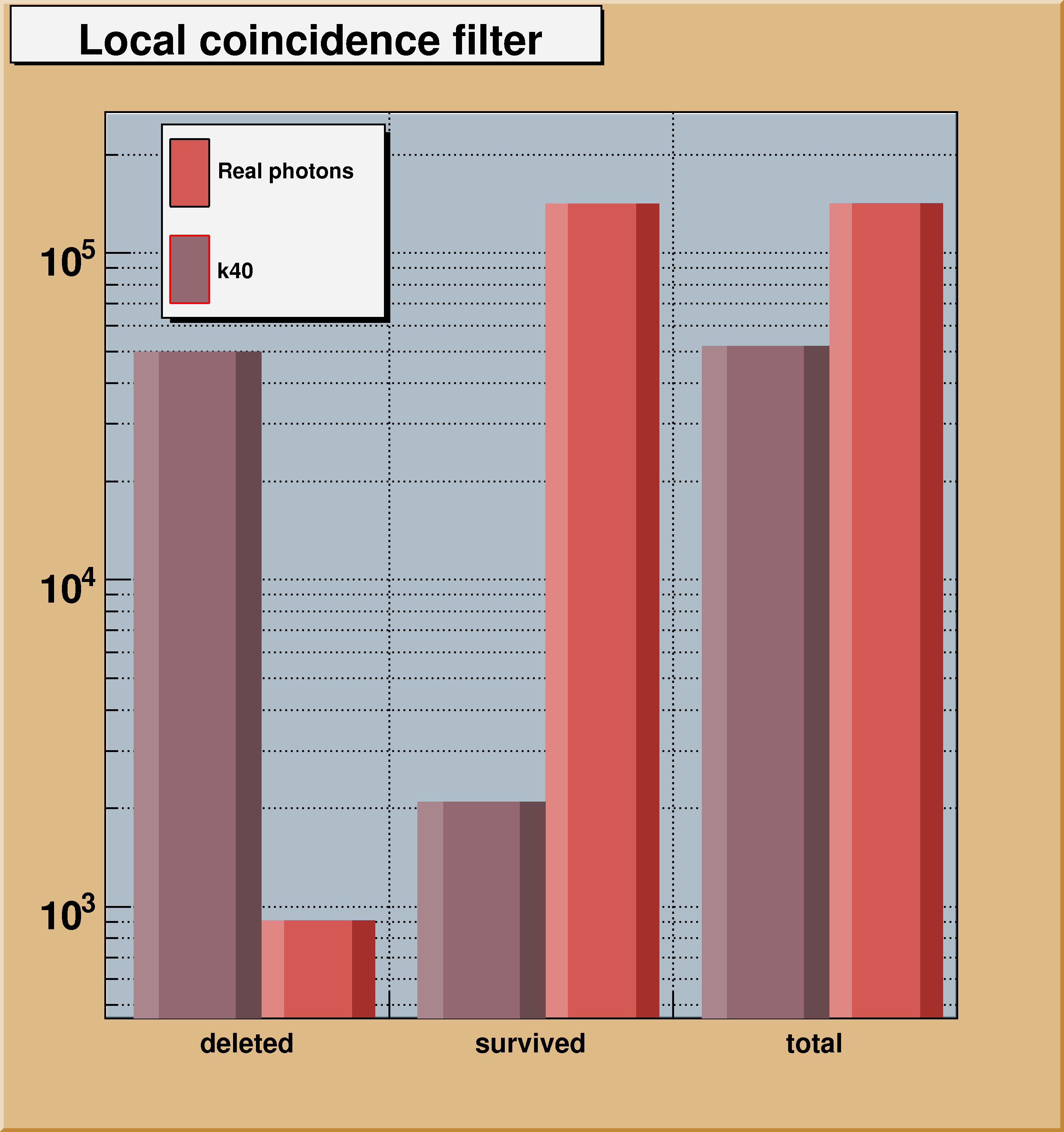
  Figure 1.11: The results of the ${}^{40}\!K$ filtering-out process over all OMs with 3 or more hits plus the largest hit of each event and its closest neighbours. String distance 120 m.

• What we are left with at this stage is a series of clusters of “large” OMs, together with isolated hits from their neighbouring OMs, which are all causally connected. Every such group of causally connected OMs is then passed through a fit with rejection method (see §1.2) with a $N$ parameter equal to $5~{}\sigma$. The resulting track is used to search again for isolated hits. The search is performed on all hits that were not used in the previous steps and which are within $~{}2$ absorption lengths from the track, on the basis of the time residuals of these hits wrt the track. After the search, and if additional hits were found, a final fit with rejection at $5~{}\sigma$ is performed again.

1.3.2 Track Parameter Estimation

One of the main problems with track reconstruction is the fact that (depending on the track energy) most of the photons produced by it do not come directly from the muon, but are produced through brehmsstralung processes away from it. The result is that the errors ascossiated with the reconstruction are not expected to be gaussian in form, or equivalently, the $\chi^{2}\;$-probability distribution is not expected to be flat. The decision was taken to always pass the reconstructed track from a final constant deweight minimization, which aggravates the $\chi^{2}\;$-probability distribution (by assigning a $\chi^{2}\;$probability close to 1 or 0 for most of them), in order to obtain a more representative pull distribution for the track parameter errors. For details, see §2.1.

1.3.3 Final Track Selection

As already noted, the above procedure allows for multiple tracks to be reconstructed. In order to eliminate ghost tracks, a search is performed amongst the reconstructed tracks for common hits. In case such common hits are identified, the track with the smaller overall number of hits is deleted if more than 10% of its hits were shared with the track with the larger number of hits.

1.4 The User Point of View

Thanks to the modular construction of SeaTray, the user only has to decide about the basic parameters of the reconstruction and implement them in the driving chameleon module in a simple python script.

The parameters are:

• The names of input and output files (both *.i3 and *.root files are supported for the output)

• The names of the various containers for particles and photons (input MC particles, output reco particles, hits, pulses etc.)

• The “HitsWeightingMethod” parameter, which specifies the way hits used are going to be reweighted during reconstruction. This parameter accepts one of three possible values:

  • “constant”: This is the default. In this case the error is set by hand in the parameter “deweightval” (see below) for all the hits of the track .

  • “residuals”: The error is set by the relative time residuals of the hit vs the recotrack.

  • “deweight”: The deweight and fit method, a recursive method which calculates the hit residuals and deweights those hits that are $N\sigma$ away from the nominal value of $2\;ns$. $N$ is set by the “deweightval” parameter (see below).

• The “deweightval” parameter, which is used with the “constant” and “deweight” fitting methods above.

The “deweightval” and “residuals” methods were developped for the study of the MC data, but were not used in the results shown in this report.

1.4.1 Analysis

The analysis of the output data can be performed with the help of a series of modules that export the relevant quantities in chains of root files (see directory AnalysisUtility). A series of scripts were written in order to make plots etc (within the scripts directory).

The implementation of the boost libraries within SeaTray allows for the use of both ROOT and python (i.e.. pyROOT) scripts for the same task (see e.g. in the scripts directory files timeDiffspyROOT.py and analysis/src/analysis_tree.C).

In cases where there is need for more computational speed, a relevant C++ class can be found in AnalysisUtility, which is also implemented in a way that allows for its usage from within both python and CINT (ROOT’s C++ interpreter). For an example see EffAreaPlotsMaker and its C++ avatar useMakeEffAreaPlotsClass(), in analysis/src/analysis_tree.C and in pythonic form in angularPlotspyROOT.py.

Chapter 2 Reconstruction Performance

2.1 Reconstruction Performance

The efficiency of the reconstruction algorithm is shown in fig. 2.1. The orange line represents the energy spectrum of all MC muons that gave hits on at least 6 OMs (Čerenkov photons originating from the muon). That is the theoretical minimum of needed OMs for a reconstruction.

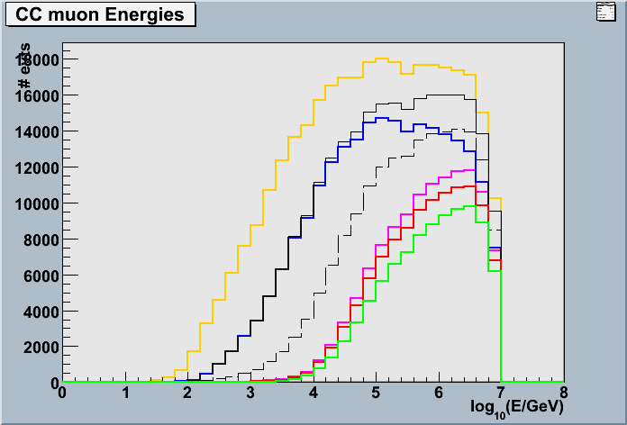
(a) The efficiency of the reconstruction vs the energy of CC muons

(b) Normalized efficiency of the reconstruction. Divided by the number of generated CC muons with more than 6 OMs hit in the sample. The fluctuation for $E<100GeV$ is due to small statistics.

Figure 2.1: The efficiency of the reconstruction vs the energy of CC muons. Orange line: Generated CC muons with more than 6 OMs hit in the sample. Black line: Generated CC muons with more than 10 OMs hit in the sample. Blue line: Contained generated CC muons with more than 10 OMs hit. Dashed Black line: Reconstructed muons with more than 6 OMs in the track. Magenta line: Reconstructed muons with more than 10 OMs in the track. Red line: Reconstructed muons with more than 10 OMs in the track, reconstructed within less than $5^{\circ}$ of the MC direction. Green line: Reconstructed muons with more than 10 OMs in the track, reconstructed within less than $0.4^{\circ}$ of the MC direction.

This spectrum is compared to the spectrum of reconstructed muons (e.g. the green line represents those tracks which contain at least 10 OMs and their direction is within $0.4^{\circ}$ of the MC direction). Out of a sample of 5,800,000 neutrinos, 492,147 were CC events with 10 or more hit OMs, 253,386 of which were contained. There were 122,302 reconstructed events with 10 or more OMs in the track, 118,930 of which originated from a CC muon.

(a) Reconstructed muons with 6 OMs.

(b) Reconstructed muons with 8 OMs.

(c) Reconstructed muons with 10 OMS.

(d) Reconstructed muons with 12 OMS.

Figure 2.2: The efficiency of the reconstruction vs the energy: Reconstructed tracks after cuts, compared with the respective numbers of “fakes”, i.e. reconstructed muons with a reconstructed direction more than $5^{\circ}$ off of the MC muon (solid black lines). All plots normalized to the number of Generated CC muons with 6 or more OMs hit in the sample.

Additionaly, fakes are shown in fig. 2.2. By “fakes” here we designate those reconstructed tracks whose direction is $5^{\circ}$ or more away from the MC direction. The differences in reconstructed and MC $\theta$ and $\phi$ angles are shown in fig. 2.3.

The cut of 10 OMs for the acceptance of a track as well reconstructed follows from plots 2.2 since it is shown there that a resonable compromise between the reconstruction efficiency and fakes is achieved for this cut. This is further corroborated by fig. 2.4, where the difference in the reconstructed and the MC neutrinos and muons is shown, before and after the cut. The overall median angle for these plots is:

• Between primary and reconstructed, before cuts, $4.55^{\circ}$.

• Between primary and reconstructed, after cut, $0.12^{\circ}$.

• Between MC muon and reconstructed, before cuts, $4.53^{\circ}$, and

• between MC muon and reconstructed,after cut, $0.11^{\circ}$.

The differential median angle between MC muon and reconstructed per energy bin is shown in fig. 2.5.

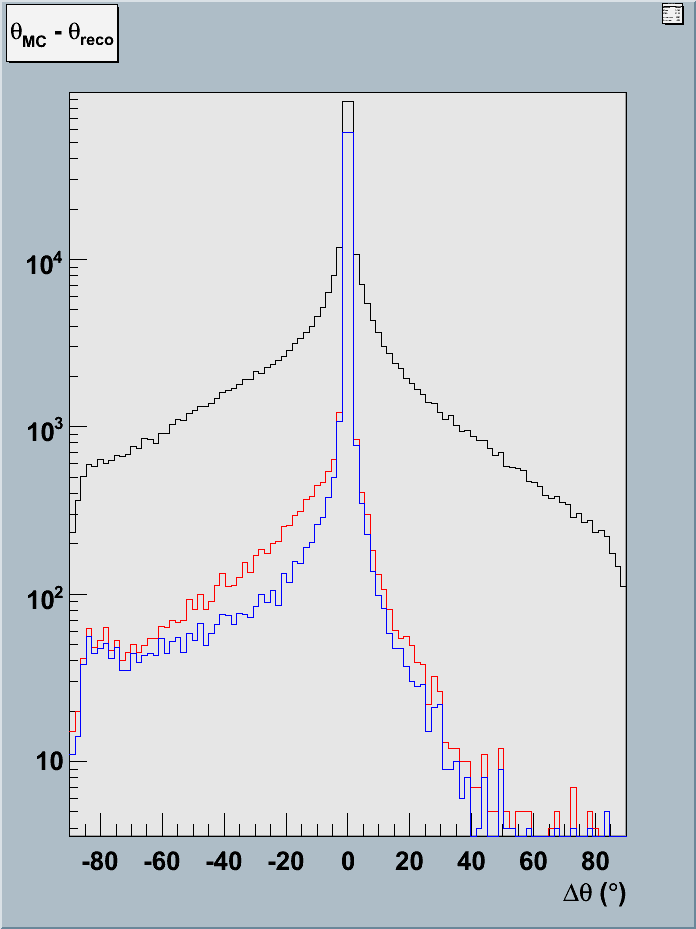
(a) $\theta$ difference.

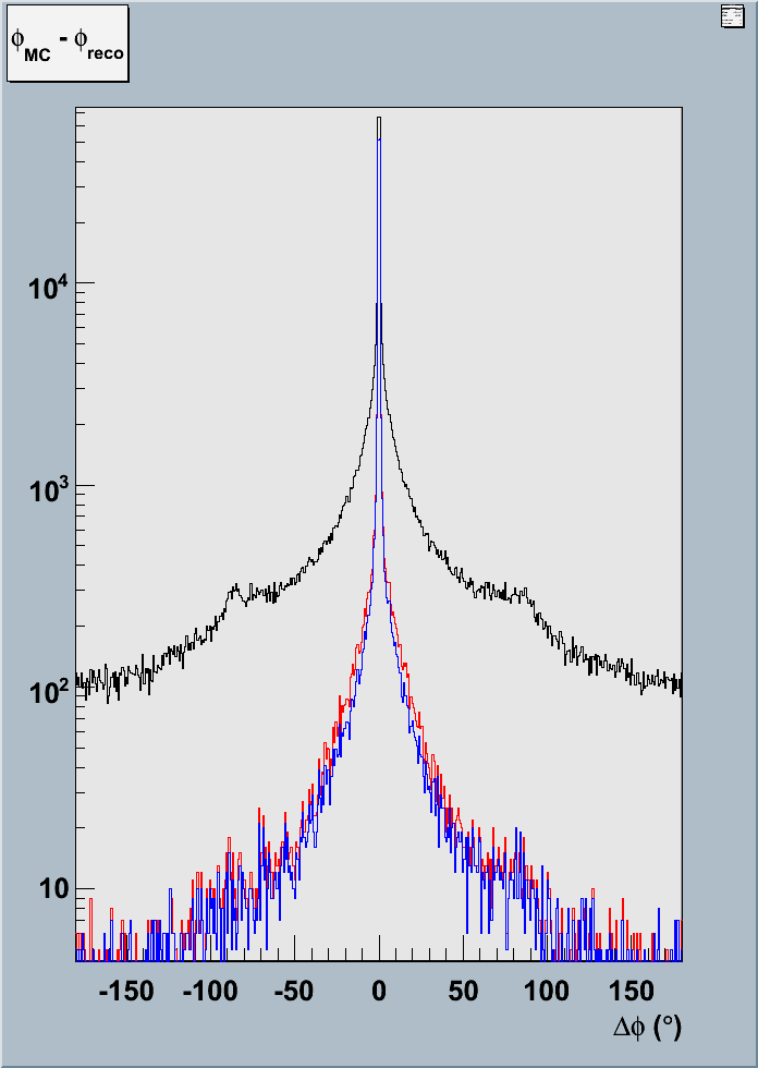
(b) $\phi$ difference.

Figure 2.3: Differences in angles between MC muon and reconstructed muon in deg. Black line: all reconstructed muons, Red line: muons with at least 10 OMs, Blue line: CC only events with at least 10 OMs.

2.1.1 A note on the asymmetry of fig. 2.3a and on ghost solutions

There is an obvious asymmetry in fig. 2.3a between up and down. This is shown separately for upcoming (fig. 2.6a), and downgoing (fig. 2.6b) tracks. This asymmetry can be possibly traced for its most part to hadronic processes, which emit undirectional spherical waves of photons. As a demonstration, in fig. 2.7, the $\theta$ differences are plotted again, but for the red line (tracks with at least 10 OMs included), we did not include those tracks that more than half of their hits are of hadronic origin. Comparison with fig. 2.3a shows immediately that the number of misreconstructed tracks has dropped by almost one order of magnitude.

The physics of the asymmetry might possibly be attributed to the detector asymmetry: OMs are not spherical symmetric (there is no top PMT). Since then OMs are slightly up-down asymmetric (one more PMT in the south hemisphere), the tracks’ $\theta$ angles (we remind that $\theta=0$ corresponds to a track coming from the nadir) tend to be slightly pulled towards the zenith when symmetric light is emmited (as is the case for hadronic processes): the OMs accept more light on their south hemispheres from a spherical wave than on their north hemispheres, thus interpreting the spherical wave as an upcoming track. Work is in progress to implement a hadronic processes module, able to identify and reconstruct correctly these tracks.

The problem of ghost solutions is of different origin. As it can be seen in fig. 2.8, where the same artificial cut on hits of hadronic origin was applied, although the tails are minimized after the cut, the kink at around $90^{\circ}$ remains. The percentage of the misreconstructed tracks around the kink (from $60^{\circ}$ to $100^{\circ}$) is 1.04% of the total reconstructed tracks with at least 10 OMs.

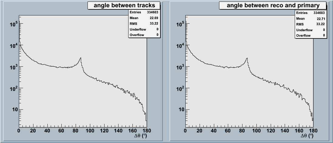
(a) Before cuts.

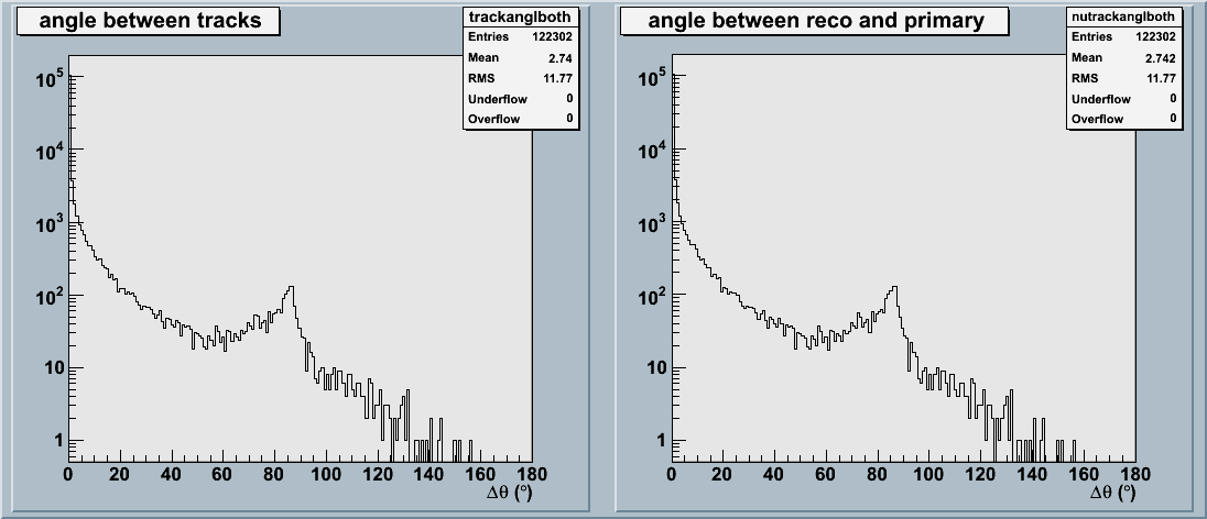
(b) After cuts (10 OMs in reco track).

Figure 2.4: Angle between reconstructed track and muon (left), track and neutrino (right).

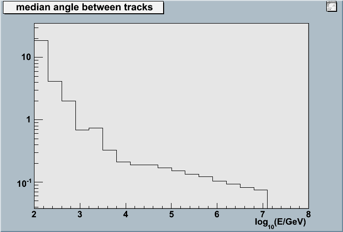
Figure 2.5: Median between reconstructed and MC muon as a function of $\log_{10}(E)$.

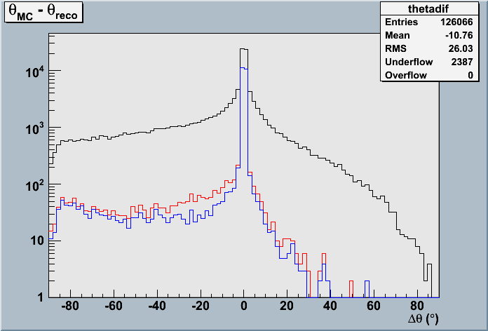
(a) $\theta$ difference, downgoing muons $z\in(0^{\circ},90^{\circ})$.

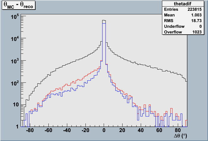
(b) $\theta$ difference,upcoming muons $z\in(90^{\circ},180^{\circ})$.

Figure 2.6: $\theta$ difference, downgoing and upcoming. Color code: see fig. 2.3

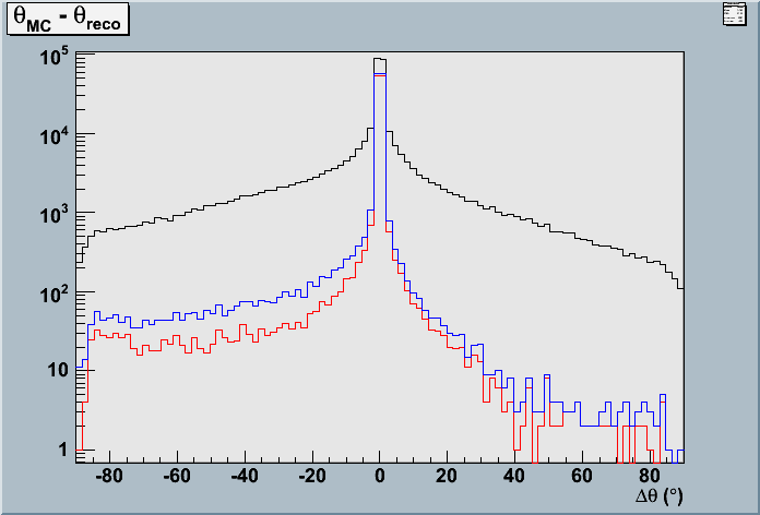
Figure 2.7: Demonstration of the up-down asymmetry (see §2.1.1). Black: MC data. Red: Reconstruction, 10 OMs. Up: Declinations.

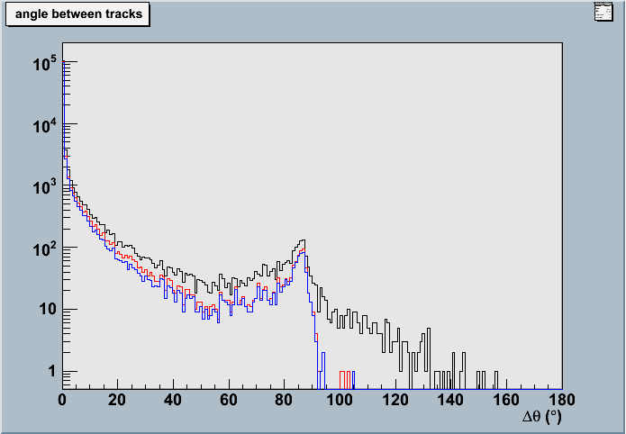
Figure 2.8: Angle between reconstructed track with at least 10 OMs hit and muon (black). The same for tracks with less than half of their hits of hadronic origin (red).

2.1.2 Quality of the reconstruction

The quality of the reconstruction can be assessed by the usual criteria of the pull distribution and the $\chi^{2}$ probability distribution. The latter is presented in fig. 2.9, while the pulls for $\theta$ and $\phi$ in fig. 2.10. These plots were produced with the reconstruction using the Constant deweight method (see §1.2), with a deweight parameter equal to 6 (see below). For completeness, we include here the $\sigma$ values for the gaussian fits of these distributions:

• $\phi$ distribution (fig. 2.10a):

  • When the $\phi$ distribution without cuts (fig. 2.10a, left) is fitted, $\sigma=1.549$. If only the peak of the distribution is fitted (from $-2$ to $2$), then $\sigma=1.097$.

  • When the $\phi$ distribution with a cut at 10 OMs (fig. 2.10a, right) is fitted, $\sigma=1.162$. If only the peak of the distribution is fitted (from $-2$ to $2$), then $\sigma=1.024$.

• $\theta$ distribution (fig. 2.10b):

  • When the $\theta$ distribution without cuts (fig. 2.10b, left) is fitted,$\sigma=1.615$. $\sigma$. If only the peak of the distribution is fitted (from $-2$ to $2$), then $\sigma=1.161$.

  • When the $\theta$ distribution with a cut at 10 OMs (fig. 2.10b, right) is fitted, $\sigma=1.209$. If only the peak of the distribution is fitted (from $-2$ to $2$), then $\sigma=1.066$.

The naturally ascociated error with each hit ($\sigma_{i}$ in eq. 1.2) is initially set equal with the time uncertainty of 2 ns (more or less equal with the time resolution available). For these plots the hits were reweighted with the rather large value of 6 ns, and the justification can be seen in plots 2.11 and 2.12, which were produced with an error value of 2 ns. The sharp peak at 0 of the $\chi^{2}$ plot 2.11, shows that we underestimate the error. This fact is also reflected to the pull distributions (figs. 2.12) whose $\sigma$ is about 3 or 4, as opposed to figs. 2.10. This in turn, is a reflection of the highly non-gaussian nature of the errors ascociated with the problem, due mainly to the multitude of different interactions involved. For example, the number of photons emitted from a track and the form of their distribution in space and time, when brehmsstralung and hadronic proceses are involved, is drastically different than the one expected from the simple formula used, eq. 1.1, which assumes that all hits are prompt photons.

Therefore, the choice was made to use a larger than expected error for the fitting process, since then the pulls’ $\sigma$ becomes 1. The application of a reasonable cut (such as 10 OMs), diminishes the tails also, which means that in this case the errors on the track parameters as calulated by the fit are more representative of the true situation (see fig. 2.10). This, in short, is the reason that a large choice for the fitting error is more adequate.

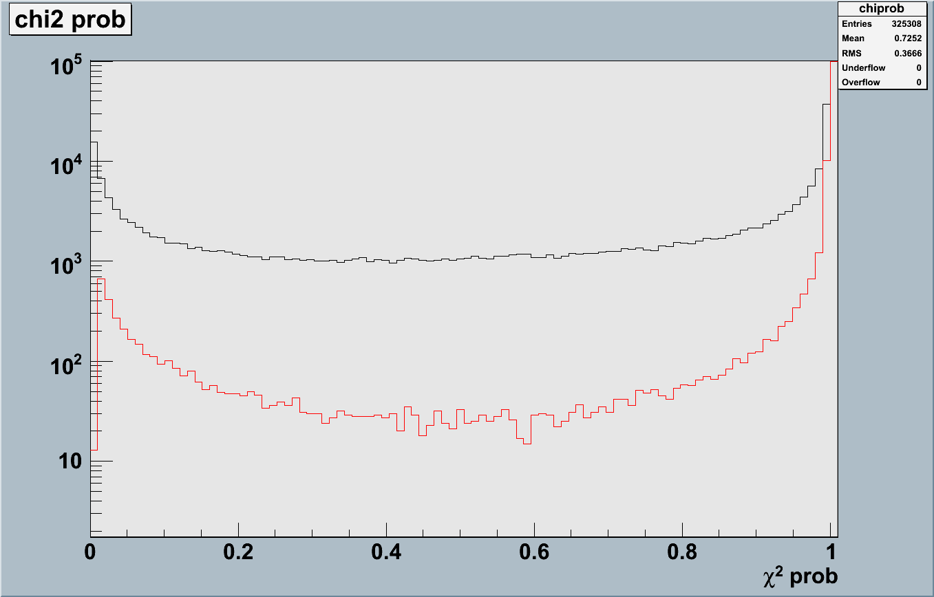
Figure 2.9: $\chi^{2}$ prob distribution. Black: All tracks. Red: reconstructed with 10 or more OMs.

(a) $\phi$ pulls ($\displaystyle\frac{\Delta\phi}{err}$).

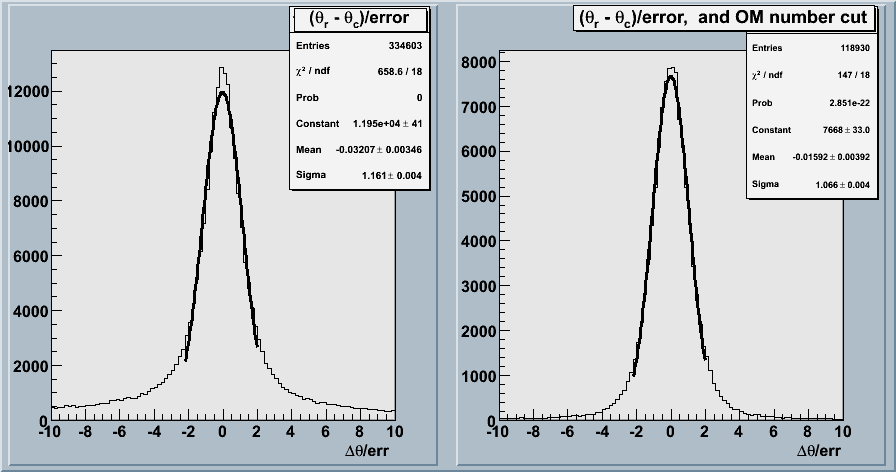
(b) $\theta$ pulls ($\displaystyle\frac{\Delta\theta}{err}$).

Figure 2.10: Pulls for $\phi,\theta$. Left: all tracks, Right: tracks with 10 OMs

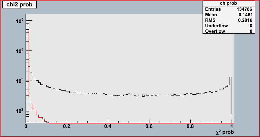
Figure 2.11: $\chi^{2}$ prob distribution for a constant deweight fitting with error = 2 (see text, §. 2.1.2). Black: All tracks. Red: reconstructed with 10 or more OMs.

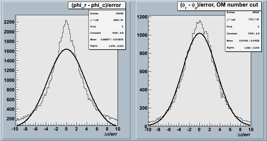
(a) $\phi$ pulls ($\displaystyle\frac{\Delta\phi}{\sigma}$).

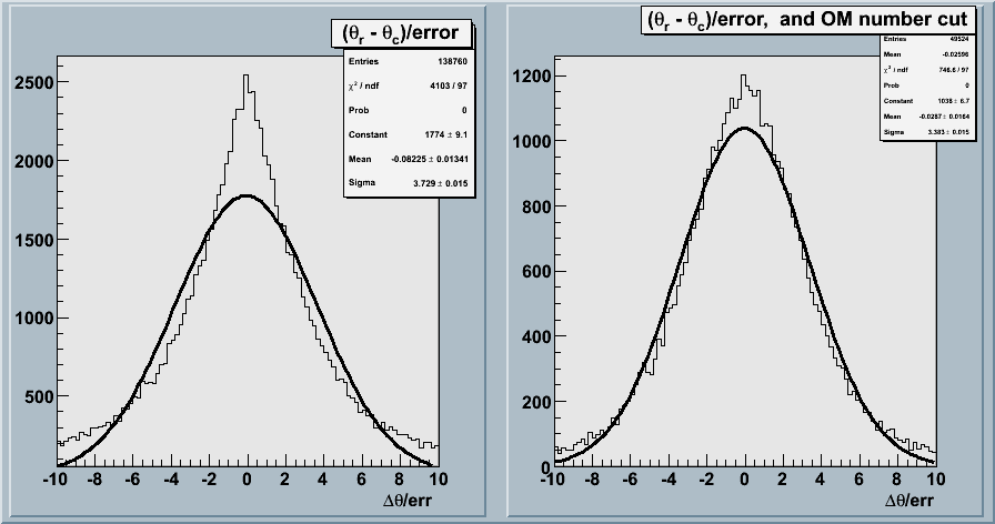
(b) $\theta$ pulls ($\displaystyle\frac{\Delta\theta}{\sigma}$).

Figure 2.12: Pulls for $\theta,\phi$ for a constant deweight fitting with error = 2 (see text, §. 2.1.2). Left: all tracks, Right: tracks with 10 OMs

The neutrino effective area vs energy is plotted in fig. 2.13, where we compare the effective area for all reconstructed tracks (blue line), to the effective area when only those tracks with at least 10 OMs are taken into account (black line). As a measure of the real efficiency of the reconstruction, we also plot (the red line) the effective area without the fakes (i.e. those tracks that are reconstructed more that $5^{\circ}$ away from the true direction).

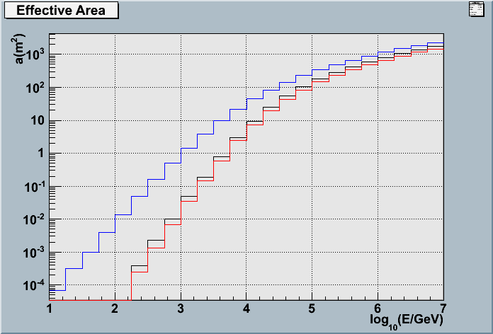
Figure 2.13: $\nu$ effective areas. Blue: all reconstructed events. Black: only events with at least 10 OMs. Red: events with at least 10 OMs, reconstructed within $5^{\circ}$ from the MC direction.

Figure 2.14: Same as 2.13, but only for upgoing muons ($z>90^{\circ}$).

Chapter 3 Depth Studies

The measure of the quality of a detector is its “sensitivity” [13], and here we expore its relation to depth. The procedure for the calculation of the sensitivity is based on the Feldman-Cousins technique [12].

The estimation of the atmospheric $\nu$ backgrounds was based on the MC files, described already in §1.1. The atmospheric $\mu$ backgrounds on the other hand, pose a difficult problem, due mainly to their large numbers – and the resulting need for resources. Within the present work, a rough MC estimation was done for them, while the more quantitative full Monte Carlo study will follow soon.

After a short description of the method we use for calculating the fluxes in the first section of this chapter, the results are presented in §3.2.

3.1 Fluxes

The first step in calculating the point source sensitivity, is the evaluation of atmospheric and astrophysical $\nu$ fluxes. The outline of the calculation is as follows:

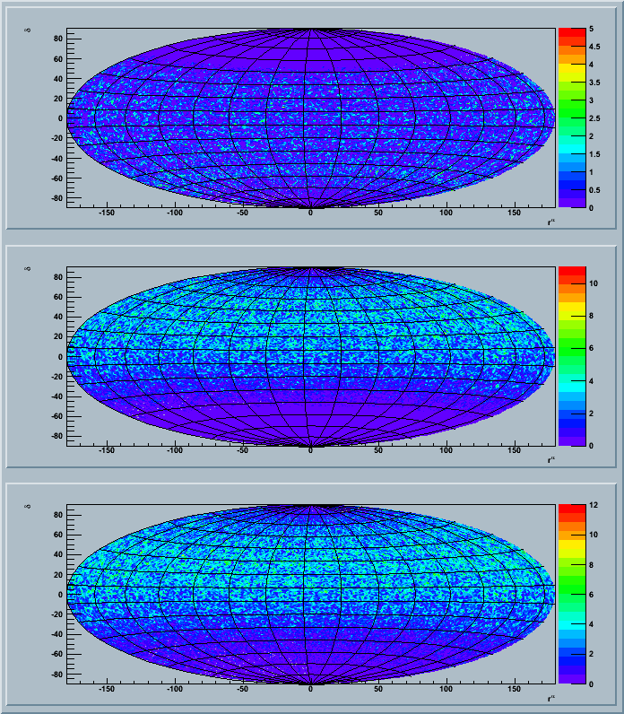
Figure 3.4: A sky map of reconstructed muons in equitorial coordinates declination $\delta$ and right ascension $r^{\alpha}$. Upper: locally upcoming muons ($z>90^{\circ}$). Middle: downgoing muons ($0^{\circ}\leq z<90^{\circ}$). Lower: Total. Not a very useful plot, but it does display nice colors.

• Extract the events’ zenith and azimuth. Calculate declinations and right ascensions (see §3.2 for a discussion of some relevant technical details and fig. 3.4 for a sky map).

• Extract the weights, as calculated from the simulation (for an explanation see [10]).

• Calculate the signal rate $R_{i}^{s}$ as

  $$R_{i}^{s}=\Phi_{\imath}^{s}\frac{O_{\imath}}{N}T,$$ (3.1)

  where $N$ the total number of events, $O_{\imath}$ the OneWeight parameter, $T$ the live time in seconds and

  $$\Phi_{i}^{s}=\frac{2.6\times 10^{-8}}{E_{\imath}^{2}}$$ (3.2)

  is the signal flux.

  

  Figure 3.1: Expected Atm. neutrino rate (as per eq. 3.3). The nature of the peaks at $\pm 1$ can be, at least partially, attributed to ghosts, see §2.1.1. Black: All reconstructed events. Blue: Reconstructed with at least 6 OMs. Red: Reconstructed with at least 10 OMs.

• Calculate the relevant background rate as

  $$R_{i}^{b}=\Phi_{\imath}^{b}\frac{O_{\imath}}{N}2T,$$ (3.3)

  where now $\Phi_{\imath}^{b}$ is a bartol flux [9] (see §1.1 and fig. 3.1). The factor of $2$ is due to the counting of both $\nu$s and $\bar{\nu}$s.

All the above factors are related to the irreducible background of atmospheric neutrinos, which is practically unchanged with depth. The only factor that depends on depth is the flux of atmospheric muons. Due to limitations of time, the full Monte Carlo study of atmospheric muon fluxes will be performed at a later stage.

From the user point of view, the task is divided in two parts. The first part is implemented in the EffAreaPlots module, which outputs the data needed for the calculation to a chain of ROOT files. The second part of the calculation is finished by a series of scripts manipulating the data (see esp. EffAreaPlotsMaker and the functions therein, and the relevant implementation scripts, e.g. analysis_plots.C and effAreapyROOT.py)

3.2 Sensitivity

We calculate the point source sensitivity by using the straightforward fixed bin method, where we use an angular bin of the order of the angular resolution (For a basic definition of terms see [8]). The main idea is that signal events will cluster around the direction of the astrophysical neutrino source under consideration (within of course the angular resolution of the detector), therefore producing an excess of events over the uniform background.

The background is made of two parts: the atmospheric neutrino part and the atmospheric muon part. The former is already included from the MC source files that were reconstructed. For the latter, a full reconstruction is not easy to be performed because of time and CPU constraints (work is underway in this direction). Until the inclusion of the full Monte Carlo data for the atmospheric muon fluxes, a general argument can be used: On one hand, the atmospheric muon intensity, as a function of sea depth, is a well documented quantity (see e.g. [1], (fig. 1-3) and discussion thereafter, or [3], fig. 15). On the other, the number of expected atmospheric muons is already given from the existing simulations. From a preliminary study of atmospheric muons at 3500 m, using the program mupage, the estimated muons that reach the detector would be of the order of $8\times 10^{9}$ events per year. This number is corroborated by (fig. 1-3) of [1], for a detector of approximate surface $1km^{2}$.

The detector produces fakes (here the word “fakes” signifies downgoing events that were misreconstructed as upcoming) at a known percentage of input events. In fig. 3.3a the ratio of misreconstructed events over the total produced downgoing MC neutrino events is shown. This ratio can be used for an evaluation of the number of misreconstructed atmospheric muons, since their energy spectrum, as a function of depth, is known. The result of this exercise is shown in fig. 3.3b.

Figure 3.2: Energy spectrum of atm $\mu$’s. Red: Depth = 5000m. Black: Depth = 4500 m. Blue: Depth=3500 m.

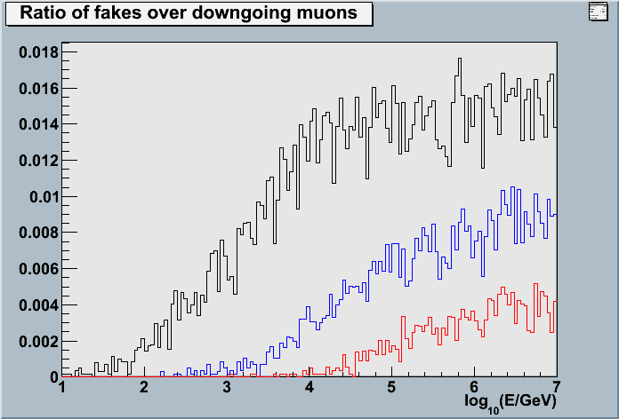
(a) Ratio of misreconstructed “fakes” over total number of MC events.

(b) Expected atm muon “fakes” over one year period.

Figure 3.3: Black: All reconstructed events. Blue: Reconstructed with at least 6 OMs. Red: Reconstructed with at least 10 OMs.

The total number of estimated fakes, at 10 OMs cut, is 94754, for a live time of one year. For a uniform distribution of the fakes over the whole lower part of the sky and an angular bin of radius $0.4^{\circ}$, this is reduced to 2.3 fakes per bin per year. It should be noted that, due to low statistics, the number of fakes is overestimated slightly (observe the fluctuations around $10^{3}GeV$ in fig. 3.3b), and averaged over the whole sky, something that is expected to be amended in the near future, after a complete reconstruction of the full data set.

As a comparison to the above number, the mean number of expected atmospheric $\nu$ background events per angular bin of $0.4^{\circ}$ per year is 4.4.

These numbers are in good general agreement with the relevant MC simulations published so far: see e.g. fig. 3.6, where the atmospheric muon intensity at 3500 m is of the same order of magnitude as the neutrino background. As a qualitative rule then, one can extrapolate the information about the atmospheric background from its two sources, calculating the total background (Atm $\mu$’s + Atm $\nu$’s), as follows: If at 3500 m, the $\mu$-background is expected to be on the average half the $\nu$ background, then at 2500 m, their ratio is expected to be roughly 2, and conversely at 4500 it will be 0.11 and at 5200 0.04.

The plot for the sensitivity for a cone of $0.4^{\circ}$ around the MC direction is shown in fig. 3.5. A calculation of the sensitivity of our detector for various $\mu$-background scenarios and for 2 different cuts on the number of OMs is presented in Table 3.1, for a declination of $53^{\circ}$, near the minimum. The left column is the ratio of the atm-$\mu$ background over the $\nu$ background, i.e. when this quantity is 1, there are equal numbers of $\nu$ and $\mu$ background events.

Table 3.1: Sensitivities $(GeV^{-1}cm^{-2}s^{-1}\times 10^{-10})$, with an estimated atm $\mu$ background.

atm $\mu$ backg	sensitivity, $90\%$ CL	sensitivity, $90\%$ CL
above atm $\nu$	6 OMs cut	10 OMs cut
0	6.06449	7.84659
0.5	6.38169	7.95273
1.0	6.74396	8.05637
1.5	7.0803	8.16001
2.0	7.38752	8.26084
2.5	7.67674	8.36077
3.0	7.94508	8.46023
3.5	8.20192	8.55668
4.0	8.43783	8.65312
5.0	8.87264	8.84108
6.0	9.27673	9.02472
7.0	9.67098	9.21145
8.0	10.0188	9.43918
9.0	10.3432	9.64955
20.0	13.4414	11.5359
50.0	19.335	14.9283
100.0	25.9965	18.9767

Figure 3.5: One year sensitivity at the Nestor site, for a cut at 10 OMs. Green line: no atm background. Red Line: An estimate for atm $mu$ background equal to atm $\nu$ background. Blue line: An atm $mu$ background equal to 10 times the atm $\nu$ background. For a discussion see section 3.2.

Figure 3.6: Taken from [14].

Bibliography

- [1] KM3Net: Conceptual Design Report.
- [2] Els de Wolf, Write up string designs (v 3.4, 14/10/2008), http://ireswww.in2p3.fr/elog/KM3NET_WP2/4
- [3] E.V. Bugaev et al., “Atmospheric Muon Flux at Sea Level, Underground, and Underwater”, Phys. Rev., D58, (1998) 054001, arXiv:hep-ph/9803488v3
- [4] Carmona PhD Thesis
- [5] Aart PhD Thesis
- [6] B. D. Hartmann, “Reconstruction of neutrino-induced Hadronic and EM Showers with the Antares Experiment”, PhD Thesis, Erlangen, 2006
- [7] S. Kuch, “Design Studies for the KM3NeT Telescope”, PhD Thesis, Erlangen, 2007
- [8] Eberl, Th. and Tzamarioudaki, K. “Simulations for the KM3NeT TDR”, http://ireswww.in2p3.fr/elog/KM3NET_WP2/10
- [9] T.K. Gaisser and M. Honda, “Flux of Atmospheric Neutrinos”, Ann. Rev. Nucl. Part. Sci. 2002 52:153-99 (hep-ph/0203272)
- [10] http://wiki.km3net.physik.uni-erlangen.de/index.php/Neutrino_generator_weights
-
[11]
C. Kopper, PhD Thesis,
http://www.ecap.physik.uni-erlangen.de/publications/pub/
ECAP-2010-003_Kopper_Dissertation.pdf - [12] G. Feldman and R.D. Cousins, Phys Rev D, 57, 1998, p. 3873.
- [13] G. C. Hill and K. Rawlins, “Unbiased cut selection for optimal upper limits in neutrino detectors: the model rejection potential technique”, Astroparticle Physics 19,3,2003,393-402 (astro-ph/0209350)
- [14] J-P Ernenwein, Presentation at WP2 meeting, Paris 2009, http://ireswww.in2p3.fr/elog/KM3NET_WP2/8, see WP2_23_FEB_2009_1.pdf.