Three-dimensional Evolution of Solar Wind during Solar Cycles 22–24

Abstract

This paper presents the analysis of three-dimensional evolution of solar wind density turbulence and speed at various levels of solar activity between solar cycles 22 and 24. The solar wind data used in this study has been obtained from interplanetary scintillation (IPS) measurements made at the Ooty Radio Telescope, operating at 327 MHz. Results show that (i) on the average, there was a downward trend in density turbulence from the maximum of cycle 22 to the deep minimum phase of cycle 23; (2) the scattering diameter of the corona around the Sun shrunk steadily towards the Sun, starting from 2003 to the smallest size at the deepest minimum, and it corresponded to a reduction of $\sim$50% in density turbulence between maximum and minimum phases of cycle 23; (3) The latitudinal distribution of solar wind speed was significantly different between minima of cycles 22 and 23. At the minimum phase of solar cycle 22, when the underlying solar magnetic field was simple and nearly dipole in nature, the high-speed streams were observed from poles to $\sim$30^∘ latitudes in both hemispheres. In contrast, in the long-decay phase of cycle 23, the sources of high-speed wind at both poles, in accordance with the weak polar fields, occupied narrow latitude belts from poles to $\sim$60^∘ latitudes. Moreover, in agreement with the large amplitude of heliospheric current sheet, the low-speed wind prevailed the low- and mid-latitude regions of the heliosphere. (4) At the transition phase between cycles 23 and 24, the high levels of density and density turbulence were observed close to the heliospheric equator and the low-speed speed wind extended from equatorial- to mid-latitude regions. The above results in comparison with Ulysses and other in-situ measurements suggest that the source of solar wind has changed globally, with the important implication that the supply of mass and energy from the Sun to the interplanetary space has significantly reduced in the prolonged period of low level of solar activity. The IPS results are consistent with the onset and growth of the current solar cycle 24, starting from middle of 2009. However, the width of the high-speed wind at the northern high latitudes has almost disappeared and indicates that the ascending phase of the current cycle has almost reached near to the maximum phase at the northern hemisphere of the Sun. But, in the southern part of the hemisphere, the solar activity has yet to develop and/or increase.

1. Introduction

The behavior of the Sun before the transition between solar cycles 23 and 24 exhibited very unusual longest and deepest minimum of activity. At the long-decay phase, the magnetic configuration of the Sun went through remarkable changes, which were different from those observed at the corresponding previous minimum phase. For example, the number of days without sunspot was large (more than 800 days at the deep minimum phase, compared to $\sim$300 days at the minimum of cycle 22) and the fluxes of extreme ultraviolet, soft X-ray, and radio intensity at 10.7 cm reached the lowest levels. Moreover, unusually long-lasting high-speed streams from low-latitude coronal holes of open magnetic field lines and their interaction with low-speed flows from closed field corona resulted in a complex heliosphere of low speed and density. The reasons for the long duration as well as depth of the peculiar minimum have been much studied, in terms of solar interior characteristics, manifestation of sunspot, polar field strength, transmission of solar wind, shaping of heliosphere, geo-effectiveness, solar irradiance, etc. (see, e.g., Basu et al., 2010; Feynman & Ruzmaikin, 2011; Jian et al., 2011; Lallement et al., 2010; Lee et al., 2009; Lo et al., 2010; Manoharan, 2010b; McComas et al., 2008; Smith & Balogh, 2009; Tapping & Valdés, 2011; Tokumaru et al., 2010). An international campaign on ‘Whole Heliosphere Interval’ was also organized to study the three-dimensional aspects of ‘solar-heliospheric-planetary connected system’. The period of the campaign covered a part of the deep minimum phase (i.e., Carrington Rotation 2068, 20 March – 16 April 2008) and included studies from low solar photosphere, through interplanetary space, and down to Earth’s mesosphere (e.g., Thompson et al. 2011).

The extended decay of the cycle 23 and the later than expected onset of cycle 24, provided opportunity to examine the link between the solar activity and three-dimensional heliosphere. In principle, the three-dimensional view of the solar wind can be inferred by the radio remote sensing interplanetary scintillation (IPS) technique, which can provide estimates of solar wind speed and density turbulence. Several authors employed the IPS technique and studied the changes of solar wind as functions of helio latitude and distance as well as over solar cycle and compared them with three-dimensional coronal density and magnetic field structures on the Sun (e.g., Rickett & Coles 1991; Kojima & Kakinuma 1990; Manoharan 1993, 1995, 1997; Manoharan et al. 1994). Recently, based on IPS observations from STELab, a distinct decrease in solar wind speed at the high-latitude regions of the heliosphere was revealed for the solar cycle 23 (Tokumaru et al., 2010).

In the present study, the large IPS data base collected from the Ooty Radio Telescope, operated by Radio Astronomy Centre, Tata Institute of Fundamental Research, India, at 327 MHz (Swarup et al. 1971), has been employed to analyze the three-dimensional distributions of solar wind density turbulence and speed at different levels of solar activity during 1985–2011. It is the detailed study of preliminary results presented in a conference proceeding (Manoharan, 2010b) and covers more than 2 solar cycles. The careful examination of consequences of various levels of Sun’s activity embedded in the solar wind gives the insight into the fundamental physical processes involved in shaping the heliosphere. The paper is structured as follows: a brief description of IPS observation is given in Section 2. The next section covers the results on distribution of density turbulence at different phases of solar cycles 22–24. The latitudinal changes of solar wind speed from IPS and Ulysses spacecraft are discussed in Section 4. In Section 5, measurements obtained from near-Earth spacecraft are discussed. Section 6 summaries the results and discussion.

2. Interplanetary Scintillation

The IPS technique exploits the scattering of radio waves from a distant compact source of angular size, $\Theta\leq 500$ milliarcsec (e.g., a radio galaxy or quasar), by the density turbulence in the solar wind (e.g., Hewish et al., 1964; Coles, 1978; Manoharan & Ananthakrishnan, 1990; Kojima et al., 2004). The measurable quantity in an IPS observation is the time series of intensity fluctuations, resulting from the radio-wave scattering caused by the plasma density irregularities convected at the speed of the solar wind and it includes irregularity structure of spatial scales from about the size of Fresnel scale and down below. For example, the IPS used in this study, at 327 MHz, can probe turbulence scales below 400 km. A suitable calibration of the temporal spectrum of intensity fluctuations can provide the solar wind speed (e.g., Manoharan & Ananthakrishnan, 1990; Manoharan et al., 2000; Tokumaru et al., 1994, 2011; Yamauchi et al., 1996, 1998; Liu et al., 2010) and the scintillation index, m (e.g., Coles, 1978; Manoharan, 1993; Asai et al., 1998). The scintillation index, $m$, is a measure of electron-density turbulence in the solar wind ($m^{2}\sim\int\delta N^{2}_{e}(z)~{}dz$), along the line of sight (z) to the radio source (e.g., Manoharan 1993; Manoharan et al. 2000).

An IPS measurement therefore represents the integration along the line of sight to the radio source. However, since most of the scattering power is concentrated at the point of closest approach of the line of sight to the Sun, as given by the typical steep radial fall of density turbulence, $\delta N^{2}_{e}(R)$ $\sim$ $R^{-4}$, the IPS basically probes properties of the solar wind at the region of the closest solar offset on the source–Earth path (Coles, 1978; Manoharan, 1993). In fact, the line of sight integration can pose a problem when a short-lived solar wind transient of enhanced density turbulence and speed with respect to the ambient solar wind is studied based on a single IPS observation, which may lead to positional uncertainty along the integration path. However in the present study, the high-level of scintillation associated with solar wind transients, e.g., coronal mass ejections (CMEs), have been removed. In the case of slowly varying large-scale ambient solar wind, an IPS observation can only systematically underestimate the solar wind by $\sim$5–10% (Manoharan et al., 1994, 2000; Yamauchi et al., 1996). Moreover, when a day-to-day monitoring of IPS is made on a large number of scintillators having different lines of sight, cutting across different parts of the heliosphere, it can probe the substantial portion of the inner heliosphere. Such data sets are extremely useful to study the evolution of large-scale features of the solar wind over an extended period of time (Manoharan, 2006, 2010a, 2010b). Since the primary aim of the present study is to understand the three-dimensional changes of large-scale structure of solar wind over a long period of time (e.g., at time scales of fraction of a year to solar cycle), no attempt has been made to remove the systematic line-of-sight integration effect included in the IPS observation.

In this study, a large amount of IPS data collected during 1985–2011 from the Ooty Radio Telescope (ORT), operating at 327 MHz (Swarup et al., 1971), has been employed. This set of IPS data from Ooty probed the solar wind in the heliocentric distance range of $\sim$10–250 solar radii ($R_{\odot}$, 1 $R_{\odot}$ = $6.96\times 10^{5}$ km, 1 AU $\approx 215R_{\odot}$) and at all heliographic latitudes. It allowed the study of the three-dimensional evolution of the heliosphere over solar cycles 22 to 24. It may be noted that before the upgrade of the feed system of the ORT around middle of 1992, everyday IPS measurements were limited to a small number of radio sources ($\sim$40–50 radio sources). The increased sensitivity of the upgraded system however enabled the observations of $\sim$300 sources per day and this source count steadily increased to the present monitoring of a grid of more than 1000 sources per day. Currently, the ORT is being upgraded and the number of IPS sources observed per day is expected to increase by $\sim$4 to 5 fold by the end of this year (Prasad & Subrahmanya 2011). The regular monitoring of IPS so far made at Ooty covers an extended period of more than 2 solar cycles and it has led to the detection of more than 3500 scintillating sources at 327 MHz, over the entire right ascension range. Results on compact component structure of these sources are in preparation (Manoharan, 2012).

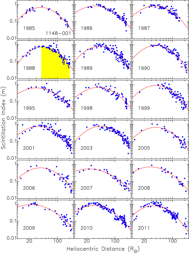
Figure 1.— Scintillation index as a function of distance from the Sun for the radio quasar 1148-001 measured from the Ooty Radio Telescope, operating at 327 MHz, over the years 1985–2011. The peak of $m-R$ curve, close to unity, shows that the radio quasar 1148-001 is compact, which in fact has an equivalent diameter of $\sim$15 milliarcsec. In each plot, the best-fit to the data points is shown by a continuous curve. The shaded portion shown on the plot of year 1988 indicates the radial distance range over which the area has been computed as given in equation 1.

3. Solar Cycle Changes of Solar Wind Density

3.1. Scintillation Index and Large-scale Density Turbulence

The degree of interplanetary scintillation is given by the scintillation index, m = rms of intensity fluctuations/mean intensity of the source, which is a measure of density turbulence in the solar wind, ($m^{2}(R)\sim\int\delta N^{2}_{e}(R)~{}dR$). Figure 1 shows the scintillation index measurements made with the Ooty Radio Telescope at 327 MHz in the heliocentric distance range of 10–250 $R_{\odot}$ on a compact radio quasar 1148-001, for selected years between 1985 and 2011. The above radio quasar has a compact component of size $\sim$15 milliarcsec (Manoharan et al., 1995). As indicated by the peak value of the scintillation index close to unity, the compact component of the above source contains more than 90% of its total flux density. It is to be noted that for a given radio source, the entire scintillation index profile, $m(R)$, is attenuated by the brightness-distribution function associated with the size of the scintillating component. Therefore, the peak value of scintillation can vary between unity and null, respectively, for an ideal point source and a non-scintillator (Coles, 1978; Manoharan et al., 1994; Manoharan, 2006). Since in the above plots, the enhanced scintillations caused by intense solar wind transient events (e.g., coronal mass ejections, refer to Manoharan et al. 2000) have been excluded, these plots represent the average condition of the ambient density turbulence of the heliosphere at different phases of solar cycles 22–24. Moreover, the radio quasar 1148-001 is an ecliptic source and its IPS measurements are confined to the equatorial region of the heliosphere. Therefore, Figure 1 represents solar wind changes occurred in the equatorial belt of the heliosphere.

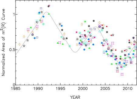
Figure 2.— The area under $m^{2}(R)$ profile (equation 1) plotted as a function of year. The area has been computed in the weak-scattering region in the distance range of 40–200 $R_{\odot}$, as indicated by the shaded area shown in Figure 1 (refer to 1988 plot). Different symbols correspond to different scintillating sources. These are strongly scintillating sources, having equivalent diameter $\leq$100 milliarcsec and their compact components contain more than 50% of the source total flux density. The continuous line is the segment-wise best fit to the data points. It is clear from the plot that the deepest minimum of of the solar cycle 23 is revealed by the lowest level of density turbulence around middle of 2008.

In Figure 1, the best-fit to the data points is shown by a continuous curve. As shown in the figure, the level of scintillation as the Sun is approached, increases to a peak value near a distance of $R\approx 40~{}R_{\odot}$, and then decreases for further closer solar offsets, where the scattering becomes strong and saturated (e.g., Manoharan 1993). The turnover point of the scintillation index moves close to the Sun as the observing frequency is increased. However for a given observing frequency, it depends only on the level of turbulence. In the above log-log ‘$m$-$R$’ plots shown in Figure 1, the peak value of scintillation index increases or decreases, respectively, in tune with maximum or minimum of solar activity. However, in order to infer the global characteristics of density turbulence in the heliosphere, the area under the best fit $m^{2}(R)$ profile has been computed for several scintillators as given by,

$$A=\int_{R=40R_{\odot}}^{R=200R_{\odot}}m^{2}(R)~{}dR.$$ (1)

For each source, the area has been computed in the weak-scattering regime ($R$ in the range $\approx 40-200R_{\odot}$). Since most of the scattering power is contained within $\sim 200~{}R_{\odot}$, the above summation provides an average quantitative estimate of the large-scale density fluctuations in the inner heliosphere of radius $\sim$0.2–1 AU over a period of about 6 months. Figure 2 shows the area of $m^{2}(R)$ curve plotted against the year for 12 compact scintillating sources. These sources have been selected on the criteria: (i) strong scintillator having the compact component of size $\Theta\leq 100$ milliarcsec, (ii) more than 50% of the total flux density of the source lies in the compact component (or the peak of the scintillation index curve is $\gtrsim$0.5), and (iii) observations of these sources fall in the ecliptic plane (i.e., in the equatorial region of the heliosphere). For each source, the computed area has been normalized by its average fraction of scintillating flux density (i.e., the ratio between the average of scintillating component flux obtained from all the available observations over the period between 1985 and 2011 and the total flux density of the source), which is a value between unity and 0.5, respectively, corresponding to an ideal compact source and a marginally broad source. In Figure 2, the data points in a year show scatter along the vertical axis and it is due to the changes in large-scale solar activity from one source to the other. Nevertheless, a smooth curve has been obtained by making segment-wise least-square fit to the data points (refer to thin line in Figure 2) and the solar cycle changes are evident in the plot. The large-scale density turbulence gradually increases from the minimum phase of the solar cycle 22, around 1986, and peaks near the consecutive maximum around the year 1991. A reduced plasma turbulence of $\sim$70% level is observed at the minima of both cycles 21 and 22, respectively, around 1986 and 1996. However, the density turbulence levels at the maximum and minimum of the cycle 23, respectively around 2002 and 2008, are observed to be lower than the corresponding values observed in the cycle 22. A decreasing trend in the turbulence level is observed from the year 1990 to 2009. At the transition between cycles 23 and 24 (i.e., between years 2008 and 2009), the density turbulence attains the lowest value of the solar cycle 23. A significant broad peak seen in density turbulence around the year 2003 is likely to be associated with the co-rotating interaction regions (also refer to Figure 4), which are caused by the persistent mid-latitude coronal holes on the Sun (Manoharan 2010b; Abramenako et al. 2010)

3.2. Radial Dependence of Density Turbulence

In the weak-scattering region at $R>40~{}R_{\odot}$ (refer to Figure 1), the gradual decrease in the scintillation with distance from the Sun is linearly related to the typical radial fall of density turbulence, $m^{2}\sim\int\delta N^{2}_{e}(R)~{}dR\sim\int C^{2}_{N}(R)~{}dR$, and from several scattering observations in the inner heliosphere, it is shown to follow the form, $\delta N^{2}_{e}(R)\sim R^{-4}$ (e.g., Manoharan, 1993; Coles et al., 1995; Coles, 1996). Thus, the quantity $C^{2}_{N}(R)$ is the measure of mean-square relative fluctuation in plasma density, $N_{e}(R)$, and it scales the spatial spectrum of density turbulence, $\Phi(q,R)=C^{2}_{N}(R)~{}q^{-p}$, where $q$ is the three-dimensional wavenumber. In the case of undisturbed solar wind, the spectrum takes the form, $\Phi(q,R)\sim q^{-3.3}$ and it gets attenuated at the high-wavenumber portion by the dissipative-scale (or inner-scale) size increasing linearly with heliocentric distance, $S_{i}\approx(R/R_{\odot})^{1.0\pm 0.1}$ km at $R\leq 100R_{\odot}$ (Manoharan et al., 1988; Coles & Harmon, 1989; Manoharan et al., 1994; Yamauchi et al., 1998). However, at larger distances from the Sun, $\sim$100–200 $R_{\odot}$, the inner scale tends to stay at a constant value of $S_{i}\approx 100$ km (Manoharan et al., 1988, 1994). The inner-scale cutoff is attributed to occur near the ion (proton) inertial scale, which is determined by the local Alfven speed and ion cyclotron frequency (e.g., Coles & Harmon, 1989; Coles et al., 1991; Manoharan et al., 1994). Therefore, the contributions to the overall turbulence spectrum include magnetic fluctuations (associated density structures) and density fluctuations and their radial changes as a function of scale size.

For example, using log-log plots shown in Figure 1, the radial dependence of scintillation can be obtained from the linear slope of $m-R$ curve at distances $>$40 $R_{\odot}$. Thus, the radial dependence of scintillation, $m=m_{0}R^{-\alpha}$ ($m_{0}$ is the scintillation index at the unit distance from the Sun), corresponds to changes in density turbulence with heliocentric distance. The $m-R$ curves of compact sources used in Figure 2 have been employed to estimate the radial fall of density turbulence. For each year, the weak-scattering portion of $m-R$ curve (at distances $\geq 50~{}R_{\odot}$) has been fitted with a least-square straight-line fit. The magnitude of slopes ($\alpha$) obtained from all the sources vary between 1.7 and 2.1, with an average of $\sim$1.8. In the period considered between 1985 and 2011, the slopes do not show significant changes in correlation with the solar cycle. However, marginal changes are observed in the radial dependence of density turbulence between periods before 2003 and later. In the prolonged minimum phase, after the year 2003, the radial fall shows an average indolent (or slow) slope of $\alpha\approx 1.7$ and a steeper slope (i.e., $\alpha\approx 1.9$) is observed for years before 2003, i.e., over the period of cycle 22 and until about the maximum of cycle 23.

As it was stated in Section 3.1, the integration along the line-of-sight would reduce the radial power by one unit (Readhead et al. 1978; Manoharan 1993). Therefore, the ‘distance-density turbulence’ relationship, $\delta N^{2}_{e}(R)\sim R^{-\beta}$, is related to the slope of the scintillation index curve by $2\alpha+1=\beta$. The steep slope observed, $\alpha\approx 2.1$, indicates that the density turbulence falls off rapidly with distance, which is about $\delta N_{e}(R)\sim R^{-2.6}$. Whereas the value of shallow slope, $\alpha\approx 1.7$, suggests a typical $R^{-2.2}$ dependence, which is close to the symmetrically expanding solar wind. These results are in agreement with the earlier findings obtained for the solar cycle 21 (Manoharan, 1993; Coles et al., 1995; Coles, 1996). The marginally less rapid slope observed in the long-deep minimum phase, $R^{-2.2}$ in comparison to the average steep slope of $R^{-2.3}$, indicates that the slow fall of solar wind is likely linked to the energy and mass fluxes associated with the solar wind originating at the base of the corona and its interaction with the background flow in the inner heliosphere. Thus, the excessive turbulence is possibly due to the interacting flows at $R>100R_{\odot}$, largely due to mid and low latitude coronal holes, which in fact persisted in the long-decay phase.

However, the mechanism of observed rapid fall in the range, $\delta N^{2}_{e}(R)\sim R^{-(\beta\approx 4~{}{\rm to}~{}5)}$, and its possible influence beyond 1 AU are required to be addressed. For example, a study of radial dependence of density turbulence by Bellamy et al. (2005), based on Voyager 2 spacecraft data, has shown much lesser fall in the outer heliosphere. Below 30 AU, small slopes of $\beta$ = 2.3$\pm$0.9 and $\beta$ = 3.3$\pm$0.9 are reported, respectively, for 96-s and 192-s sampling intervals, which correspond to spatial scales of about one to two orders of magnitude larger than scales probed by the IPS observation. The above study also reveals that the level of $C^{2}_{N}(R)$ drastically changes with the employed sampling rate (i.e., probed scale size of turbulence). Thus, at distances beyond 1 AU, the radial dependence of turbulence spectrum, $\Phi(q,R)$ (also $C^{2}_{N}(R)$), shows flattening, enhancement, and dissipation as function of spatial scales and tends to be independent of regular expansion of the background solar wind (Bellamy et al., 2005; Hunana et al., 2008; Zank et al., 1996).

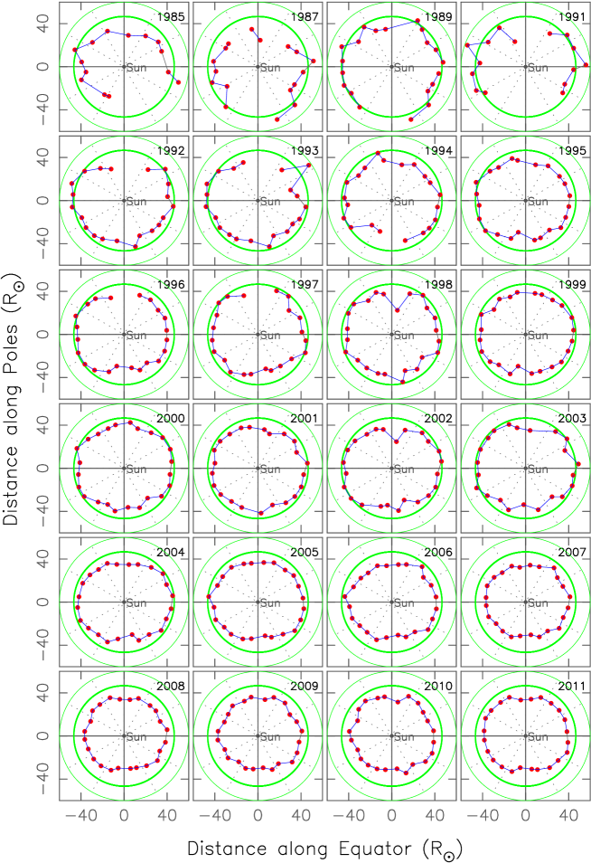
Figure 3.— Constant $\delta N_{e}(R)$ contours plotted on ‘north-east-south-west-north’ polar diagram for selected years between 1985 and 2011. The last plot includes data up to November 2011. In each plot, reference circles are drawn, respectively, at radii 45 and 60 $R_{\odot}$ and 30-degree latitude sectors are shown by dotted lines. During 2008-09, the scattering diameter of the corona has shrunken to the smallest size and the solar activity touched the deepest minimum of solar cycle 23. The increase in the diameter of the contour in the year 2011 evidently reveals the progression of cycle 24.

3.3. Scattering Diameter of the Corona

The routine monitoring of IPS at Ooty, on a large number of compact radio sources during the period 1985–2011, has been used to estimate constant density turbulence contours at different phases of solar cycles 22 to 24 (Manoharan, 2006, 2010b). At an observing frequency, the peak of the scintillation curve, m–R (refer to Figure 1), depends on the fixed level of density turbulence and the heliographic coordinates of several peaks distributed around the Sun are useful to find the contour of the constant (or same) level of density turbulence (${\delta N_{e}(R)}$) in the heliosphere (e.g., Manoharan 1993; Coles 1978). At 327 MHz, the turnover of scintillation occurs around $\sim$40$R_{\odot}$. In Figure 1, although these are log-log plots, a careful examination reveals that the peak point of the scintillation curve (i.e., constant value of ${\delta N_{e}(R)}$) moves close or away from the Sun, respectively, at the minimum or maximum phase of the solar cycle. Therefore at 327 MHz, the estimation of $m-R$ curves of several ecliptic and out-of-ecliptic sources in a year and their corresponding peaks located at different latitudes (as well as heliocentric distances) can provide the trace of constant level of density turbulence around the Sun in the distance range of 30–50 $R_{\odot}$.

In a year for each source, the average peak of the scintillation and its heliographic coordinates are obtained and plotted around the Sun on a north-east-south-west-north radial diagram. As shown in Figure 3, the latitude-bin average of peaks at different latitudes and the line joining them can provide the constant density turbulence contour around the Sun (e.g., Manoharan 1993). Although this figure includes average constant ${\delta N_{e}(R)}$ contours for selected years between 1985 and 2011, the data coverage was sparse during the solar cycle 22. It was due to the fact that in the early days observations at Ooty less concentration was given to IPS below 50 $R_{\odot}$ and measurements were mostly limited to the weak-scattering regime, $>50R_{\odot}$. However, starting from the second half of cycle 22, IPS measurements were carried out over the full distance range of 10–250 $R_{\odot}$ and they enabled the determination of transition of scintillation for sources favorably positioned with respect to the Sun. In Figure 3, the mean traces of constant level of density turbulence indicate that in general at the polar regions, the constant level of turbulence is observed closer to the Sun than at the equatorial region. It is in agreement that at the descending phase of the activity, the low-density (i.e., high-speed) streams from coronal holes fill the polar regions, leading to low level of density turbulence and constant ${\delta N_{e}(R)}$ contour moves close to the Sun to compensate the fall in scattering power at the high-latitude region of the corona. However, as the Sun approaches towards the minimum of activity, the size of the coronal hole increases and extends to mid latitudes (Manoharan, 1993; Coles et al., 1995; Coles, 1996). In such a phase, the density turbulence contour takes a shape close to an ellipse, in which the contour at the mid-latitude part also moves close to Sun (Figure 3, refer to 1994–96 plots). In the ascending phase, the ratio between poleward and equatorial diameters however gradually decreases from minimum to maximum phase of the cycle (e.g., Manoharan 1993; Coles et al. 1995) and the ratio of diameters tends to unity at the maximum of the cycle. The solar wind flow thus attains a spherically symmetrical flow, as revealed by the almost circularly symmetrical distribution of streamers at the maximum phase of the corona observed during the total solar eclipse (e.g., Koutchmy et al. 1992).

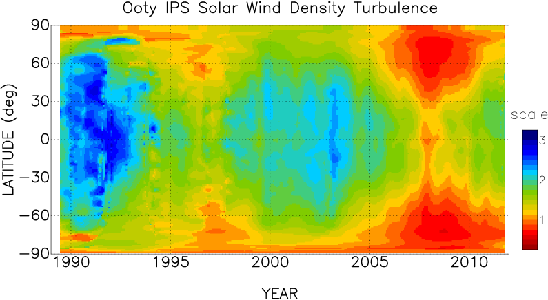
Figure 4.— Helio latitudinal distribution of solar wind density turbulence as a function of year. This image has been made by allowing data in the heliocentric distance range of 75–125 R_⊙ and it shows the condition of the heliosphere at the midway between the Sun and Earth. The distribution of density turbulence shows remarkable change between minima of solar cycles 22 and 23.

The interesting result of this study is that after about the year 2003, the overall scattering diameter of the corona has gradually decreased with respect to the center of the Sun and a given level of turbulence has steadily moved close to the Sun at all latitudes. The diameter of contours during the years 2007–2009 appear symmetrical, but much smaller than the contours observed in the cycle 22. The typical radial dependence of turbulence, $C^{2}_{N_{e}}(R)\sim R^{-4}$ to $R^{-4.4}$, suggests that the scattering has remained nearly same at low-latitude regions between 1995 and 2003, but, steadily decreased to $\sim$60% level around middle of 2009, where the deepest minimum of cycle 23 was observed. The shrinking of scattering diameter of the corona is in agreement with the measured level of scintillation displayed in Figure 2, which also shows the overall gradual reduction in scattering power between the years 1986 and 2010. The equatorial diameter starts to increase between 2010 and 2011, indicating the onset and progress of the solar cycle 24. The steady and significant long-term trend of shrinking of scattering power of heliosphere means a natural reduction in supply of mass and energy at the low corona.

3.4. Latitudinal Distribution of Density Turbulence

At Ooty, IPS on a source is measured at different solar offsets. For each source, the scintillation index plot ($m(R))$ in a year, as plotted in Figure 1, can be least-square fitted with an average curve. The ratio between the observed and expected (or fitted) indexes at a given heliocentric distance, g = observed scintillation/average expected scintillation, can be used to assess the level of density turbulence of the slowly varying solar wind structures in comparison with the ambient (or background) solar wind plasma (Manoharan, 2006). The above normalized scintillation index, g, is independent of systematic fall of m with solar offset and source-size attenuation. For example, a value of the normalized index close to unity ($g\approx 1$) represents the undisturbed (or background) condition of the solar wind, $g>1$ corresponds to the enhanced level of density turbulence, and, $g<1$ indicates the reduction of turbulence in the solar wind. An IPS measurement is therefore sensitive to detect even a small fractional change in the density turbulence and the routine monitoring of IPS on a grid of sources can easily detect the large-scale structures over a given period of time (Manoharan, 2006).

For each source, the best fit to $m-R$ curve of a given year is estimated and it is used to eliminate the intense transients caused by the CMEs. The transients removed data sets of a given source, available for the period between 1985 and 2011, are then combined and the overall least-square fit is computed. Thus, the value of g obtained from the fitted curve and each observed scintillation index allows an easy comparison of levels of turbulence measured on a number of IPS sources at different time periods and it enables the detection of slowly varying large-scale density structures in the solar wind. Figure 4 displays the ‘latitude–year’ plot constructed from the normalized scintillation index estimates obtained from the continues Ooty IPS measurements between 1989 and later part of 2011 (Manoharan et al., 2000, 2001; Manoharan, 2006). In a broad sense, this plot resembles the ‘sunspot butterfly’ diagram and reveals the major large-scale structural changes of the heliosphere occurred through solar cycles 22 to 24. Since the density turbulence ($\delta N^{2}_{e}$) and g are linearly related only in the weak-scattering region, which typically occurs at distances $>$40 $R_{\odot}$ for IPS at 327 MHz (e.g., Manoharan 1993), in the above image we have employed measurements made in the distance range of 75–125 $R_{\odot}$. Therefore, the above latitudinal plot represents the density turbulence of the inner heliosphere at a radius of about midway between the Sun and the Earth.

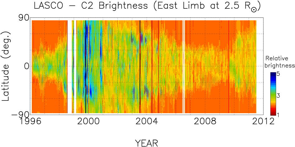
Figure 5.— Helio latitudinal distribution of Thomson-scattered brightness observed at 2.5 R_⊙ by the LASCO-C2 coronagraph (Brueckner et al., 1995), as a function of year. The brightness represents the coronal density. At the minimum of solar cycle 22 around the year 1996, the density above the equatorial closed-field corona was much intense as well as narrow in latitudinal spread, suggesting a nearly-dipole configuration of the coronal field. Whereas, in the long-decay minimum phase, the density was rather low along the equatorial belt and it occupied broader latitude range. These results are in agreement with IPS measurements.

The above density turbulence image shows several interesting features. The high-latitude streams from coronal holes are always associated with low-density turbulence (Rickett & Coles, 1991; Manoharan, 1993). The drifting of large-scale structures from high to low latitudes, seen as intense vertical bars (refer to Figure 4, between years 2000 and 2004), are likely due to the migration of medium to large-size coronal holes from polar to low-latitude corona. The high-speed streams from these coronal holes interact with the low-speed wind, causing the density compression and resulting in increased turbulence in front of the high-speed flow. The interaction is rather efficient at low and mid-latitudes, where the speed difference between low and high-speed flows is significant, but, it weakens with increasing latitude (e.g., Gosling et al. 1995). The spread of high-density features, which are limited to mid-latitude region ($\sim$$\pm$40^∘) at the minimum phase and much wider ($>$60^∘) during the maximum, are consistent with the tilt angle of the neutral line (refer to Figure 7). The neutral line on the source surface of the Sun divides regions of opposite polarities. It is swept radially outward by the solar wind and forms the heliospheric current sheet (HCS). At the time of polarity reversal, the amplitude of HCS extends to high latitudes, suggesting a complex closed magnetic field topology, resulting between the coronal holes and active regions. For example in Figure 4, the disappearance of the solar wind (Lazarus, 2000), shown by the vertical low-density structure around middle of 1999, is consistent with the complex as well as a rather closed-field corona to confine the plasma, as the Sun approaches towards the peak of the cycle 23 (Figure 7).

The other interesting feature in Figure 4 is the co-rotating interaction regions (CIRs) dominated heliosphere resulted from the persistent large coronal holes in the latitude range of $\pm$45^∘, as shown by the vertical intense density structure caused by the moderate compression during 2003–2004 (Zhang et al., 2008; Abramenako et al., 2010). In this period, each solar rotation possessed more than one heliospheric current sheet, running almost parallel to the latitude axis, increased the possibility of interaction between low- and high-speed streams. These interactions caused weak to moderate storms at the Earth during 2003, as indicated by the geo-magnetic disturbance index, Ap (refer to Figure 9).

The density distribution in the maximum phases of solar cycles 22 and 23, respectively centered around years 1991 and 2001, shows rather remarkable differences. The low- and mid-latitude regions of the heliosphere near the maximum of cycle 22 were associated with high-density structures. Whereas the large portion of the heliosphere, even at the maximum of cycle 23, was occupied by a relatively low-density plasma, as was indicated by the density turbulence contours (refer to Figures 2 and 3). It is also interesting to note large differences in low-density plasma turbulence at the polar regions near the minima of cycles 22 and 23. During years 1996–1997, the low level of turbulence was confined to latitudes above 45^∘ in the north and south hemispheres. In the prolonged minimum period, during years 2006-2009, the density was much lower than that of the previous minimum as well as it occupied a broader latitude range extending from high to low latitudes. The low-density plasma prevailed the large portion of the inner heliosphere around the unusual deep minimum phase and it is in agreement with the corresponding shrinking of scattering diameter of the corona (Figure 3). The density distribution observed after about the year 2010 indicates that the heliosphere is gradually climbing towards the maximum phase of the solar cycle 24. The rate of increase of density to high latitude in the north pole seems to be faster than that observed at the south pole, suggesting that the solar cycle 24 tends to approach a near-maximum phase in the northern hemisphere.

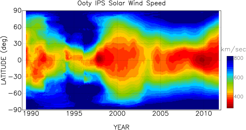
Figure 6.— (a) Helio latitudinal distributions of solar wind speed obtained from Ooty IPS data plotted for years 1989–2011. This image has been made by tracing backward/forward from the measurement location onto a sphere of radius $\sim$125 solar radii. At the minimum of solar cycle 22, the effects of high-speed wind were observed from poles up to about $\sim$30^∘ latitudes. But, in the prolonged minimum, the high-speed streams were located close to poles.

3.5. Density Distribution in the near-Sun Corona

Ooty density turbulence results are consistent with the brightness measured from the Thomson-scattered white-light in the near-Sun region. Figure 5 shows the ‘latitude–year’ image of the white-light, which is associated with the density of free electrons, measured at 2.5 $R_{\odot}$ above the east limb of the Sun, for the period starting from the launch of LASCO coronagraph to nearly middle of the year 2011 (refer to Brueckner et al. (1995) for details on LASCO coronagraph). As shown by the IPS data, the heliosphere was prevailed by low density during the prolonged minimum of the solar cycle 23. The latitudinal extents of large-scale low density structures in the mid- and high-latitude regions are also agreement with the IPS density turbulence distributions. The intense density structure observed on the IPS image, associated with CIRs generated by the mid- and low-latitude coronal holes around 2003, is represented on the LASCO image by a less-brightness stripe, which provides evidence for the low-density wind originating above the coronal hole and in particular, not yet developed interaction as well as compression at the closer solar offset. In the minimum phase of cycle 23, the long-lived coronal holes observed during 2003, might have a more direct involvement in shaping the magnetic state of corona at the deep minimum phase (Abramenako et al., 2010). The three-dimensional distribution of Lyman-$\alpha$ brightness, which reflects the ionization of the neutral gas by the solar wind, also in agreement and showed a latitudinal distribution similar to the above shown density turbulence and density images, respectively, displayed in Figures 4 and 5 (Lallement et al. 2010). The onset of the solar cycle 24 in the year 2009 and the gradual increase in the latitudinal extent of high density wind to higher latitude between 2010 and 2011 (particularly at the north-pole side) are evident in Figure 5. However, as indicated by the density turbulence (Figure 4), the southern hemisphere seems to progress slower than the northern part.

4. Solar Cycle Changes of Solar Wind Speed

For an IPS observation in the weak-scattering regime, a suitable calibration of the temporal power spectrum of intensity fluctuations, having sufficient signal-to-noise ratio (i.e., $\gtrsim$15 dB), can provide the speed of the solar wind (Manoharan & Ananthakrishnan, 1990; Manoharan et al., 2000; Tokumaru et al., 1994, 2011; Yamauchi et al., 1996, 1998; Liu et al., 2010). Figure 6 shows the ‘latitude–year’ distribution of solar wind speed estimates obtained from the IPS data collected from the Ooty Radio Telescope, as it was displayed in the plots of density and density turbulence (Figures 4 and 5). During the minimum of solar cycle 22, polar regions were dominated by high speed streams in the range $\sim$700–800 km s^-1, from open-field coronal holes and low and variable flow speeds, $\leq$450 km s^-1, were observed at the low- and mid-latitude regions of the complex/closed field corona (Phillips et al., 1995; McComas et al., 2008; Smith & Balogh, 2009). The striking features in this image are (i) confined period of minimum for cycle 22, centered around year 1996 and the high-speed wind (or the extension of coronal holes) observed from poles to mid-latitude region of $\sim\pm 30^{\circ}$, and (ii) in contrast, the effects of minimum of cycle 23 was stretched over a long-period of time and the width of the high-speed belt was limited to latitudes higher than 60^∘ in north and south poles; a deep minimum-like condition was observed between years 2008 and 2009, during when the extent of high-speed belts at the north and south poles were limited between the poles and $\sim$60^∘ latitudes. Further, the speed originating above them has been considerably reduced. The low-speed solar wind distribution, along the equatorial belt, seems to be highly variable in the range 300–500 km s^-1, and the ‘disappearance of solar wind’ (i.e., extremely low density and speed) occurred in the early part of the year 1999 as well as the coronal-hole dominance in the mid-latitude region of the heliosphere during 2003 are evidently revealed.

Figure 7 shows the smoothed plots of tilt angle of the magnetic heliospheric current sheet (HCS), and strength of polar magnetic field. For reference, sunspot number and radio flux density at 10.7 cm are also included in this figure. The magnetic field data sets have been obtained from the Wilcox Solar Observatory and the solar activity indexes are from Solar Geophysical Data Center. These plots cover a period from 1985 to the later part of 2011, i.e., solar cycles 22 to 24. The large-scale magnetic field, shown by the amplitude of current sheet during years 2004–2008, resembles a corona of complex field, but with the reduced activity. The remarkable increase in the latitudinal width of low-speed flow during the extended minimum of cycle 23 is directly linked and in good agreement with the observed polar field strength and warping of the current sheet, which is caused by the extension of global field from the Sun into the interplanetary medium. The solar wind speed distributions observed for solar cycles 22 and 23 correlate, respectively, with the polar field strength of $\sim$100 to 50$\mu T$. Thus, the magnetic field has been weak by $\sim$40–50% in the minimum phase of cycle 23 than that of cycle 22 (Figure 7). The magnetic pressure associated with the polar coronal holes consequently seems to play a significant role in the acceleration of high-speed wind. The weak field may be due to the fact that the polar field has not fully developed after the field reversal between 2000 and 2002 (Figure 7).

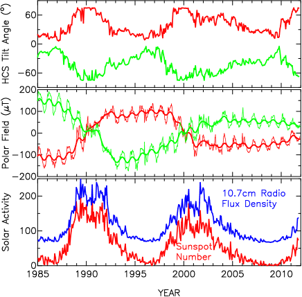
Figure 7.— The stack plot shows solar activities (i.e., sunspot number and solar radio flux density at 10.7 cm), intensity of polar magnetic field, and tilt angle of heliospheric current sheet (HCS). The reduction in the strength of the polar fields is evident after the reversal of the field around the year 2000.

It was reported that the Sun went through a period of large number of ‘sunspot-free’ days (more than 800 days between 2006 and 2009, in comparison with $\sim$300 days of ‘spotless’ days in the minimum of cycle 22). Moreover, at the extreme minimum phase of cycle 23, the solar wind distribution around the equatorial belt as well as the tilt angle (refer to Figure 7) suggest that the magnetic field of the Sun did not approach the expected dipole geometry, as it did for the minimum phase of cycle 22 (Riley et al., 2003; Tokumaru et al., 2009). The weakening of the large-scale coronal field has also been revealed by the weak emission of Fe XIV green line at $\lambda$5303 Å  (Rybanský et al., 2005). Additionally, Ulysses and near-Earth observations (Figures 8 and 9) made over the solar cycles 22 and 23 are in good agreement with speed and density distributions presented in the previous sections (McComas et al., 2008; Smith & Balogh, 2009; Lee et al., 2009). Figure 8 shows the daily averages of the magnitude of interplanetary magnetic field and solar wind speed, as measured by Ulysses spacecraft around minima of solar cycles 22 and 23. Ulysses measurements evidently show an overall reduction in field strength, density, speed, as well as the increased width of the equatorial flow and poleward shrinking of the high-speed wind for the similar latitudinal and heliodistance passes of cycles 22 and 23. The lack of sunspots activity governing the radiative energy from Sun, in combination with the weakening of the interplanetary field and turbulence, allowed the penetration of cosmic rays at the minimum phase of cycle 23 by more than $\sim$20% than at 1997–1998 period (Mewaldt el al. 2010).

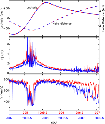
Figure 8.— Daily averages of the magnitude of interplanetary magnetic field and solar wind speed at the orbit of Ulysses as a function of year, around minimum phases of solar cycles 22 and 23. Close tracking of location of Ulysses on the heliosphere, for these two passes, clearly shows (i) significant reduction in equatorial flow widths, (ii) rapid decline in speed, and weaker field at minimum of cycle 23 than that of corresponding previous minimum of cycle 22.

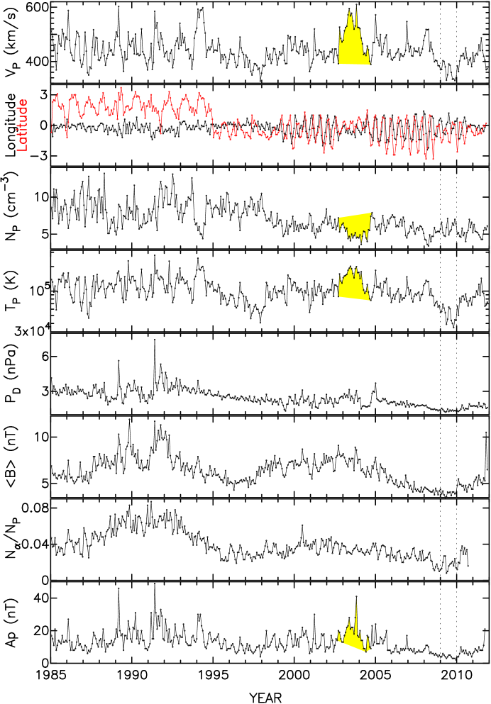
Figure 9.— Plots of 27-day average of solar wind proton speed and flow directions (i.e., latitude and longitude in degree), number density, temperature, dynamical flow pressure, magnitude of interplanetary magnetic field, and ratio of alpha particle to proton densities, as a function of year. The geo-magnetic index, Ap, is shown in the bottom plot. The yellow shades show CIR dominated period during the minimum of cycle 23. The vertical dotted lines indicates the deep minimum phase of cycle 23.

As observed in density and density turbulence plots (refer to Figures 4 and 5), the speed distribution plot (Figure 6) also shows that after the onset (i.e., in the ascending phase) of solar cycle 24, starting from middle of 2009, the changes observed in the distribution of high-speed solar wind at the north and south polar regions are different. In particular, at the later part year 2011, the high-speed belt at the northern region has moved almost close to the its pole. However, in the southern part, it has remained nearly unchanged. It suggests that the area of the northern coronal hole associated with the high speed wind has reduced and shrunk close to the north pole. In other words, the increase in the solar activity (i.e., vanishing of source of high-speed wind) is significant at the northern hemisphere and indicates nearly (or close to) the maximum phase of cycle 24. It is consistent with the yearly average values of flare index observed at northern and southern hemispheres over the year 2010, respectively, 0.26 and 0.12. The northern hemisphere of the Sun was 2 times more active than the southern hemisphere.

5. Solar Cycle Changes at near-Earth Space

Figure 9 shows the 27-day average of 1–AU measurements of solar wind proton speed and its flow directions (i.e., latitude and longitude), number density, temperature, dynamical flow pressure, magnitude of interplanetary magnetic field, and ratio of alpha particle to proton densities, observed between years 1985 and 2011. A plot of geo-magnetic index, Ap, is also included in the figure. These data sets have been extracted from the NASA/GSFC’s OMNI data base. It is evident that in the near-Earth region, the solar wind dynamical pressure started to decrease after the maximum phase of cycle 22 (after about year 1992), to a deep minimum during the years 2008–2009. Although there was a moderate enhancement in the solar wind pressure at the maximum of cycle 23, it was however nearly 40% lower than the corresponding increase observed at the previous activity maximum. In the long decay phase of cycle 23, the inter comparison of results from previous sections with 1–AU measurements of solar wind speed, proton and alpha particle densities, temperature, pressure and interplanetary magnetic field suggests that the reduction in density and magnetic energy of the solar wind streams has organized the heliosphere. Thus, the energy of the solar wind started to decrease after the maximum of the cycle 22 and continued up to the transition between cycles 23 and 24.

In Figure 9, there are two interesting periods, 1993–1994 and 2003–2004, in which the presence of equatorial coronal holes dominated the solar wind flow. They are prominently seen as enhancement in speed and temperature, and depletion in density. The period, 2003-2004, is shown in shade on plots of speed, density, temperature and corresponding geo-magnetic index. As revealed in the speed and density turbulence images (Figures 4 and 6), the corresponding interaction between the high-speed wind from low-latitude coronal hole and ambient (or background) low-speed wind has resulted in compression region and led to increase in density turbulence (refer to Figures 4 and 6). The period of coronal hole dominated low-latitude solar wind was shorter during the cycle 22 than that of cycle 23, in which the solar wind interactions have caused moderate to strong geo-magnetic activities as recorded by Ap index.

The presence of equatorial and mid-latitude coronal holes and their evolution during the years 2003–2004 have likely caused the changes observed in the flow direction of the solar wind. In Figure 9, the second plot from the top shows the flow longitude and latitude. The solar wind longitude, during years 1985 to 1999, did not show systematic variation with the activity of the Sun. Whereas the quasi-periodic oscillations of amplitude $\sim$2–4^∘ observed in the solar wind flow latitude were likely caused by the latitudinal warping of the heliospheric current sheet. In contrast, the regular variations in flow latitude and longitude ($\sim$3–4^∘) between 1999 and 2003 show that the flow direction exhibits cyclic changes in the west-north-east-south direction. The mean period of oscillation is $\sim$6 month, which indicates a cyclic behavior linked to the slow changes ($>$27-day period) of large-scale structures of the source of the solar wind. However, the above cyclic pattern of solar wind flow direction disappears between 2003 and middle of 2004, in coincidence with the duration of the high-speed wind caused by the large mid-latitude coronal hole. But, it appears back in the later subsequent time and the solar wind flow geometry changes to a reversed opposite cyclic behavior of east-north-west-south pattern.

In the ascending phase of solar cycle 23, after the year 1994, the dominance of equatorial coronal holes disappeared, the solar wind flow direction switched from largely north pointing to equatorial flow. It implies that the large-scale magnetic field averaged over a solar rotation, with respect to the heliospheric equator, has gone through a systematic reversal during the ascending phase of the solar cycle. In the case of solar cycle 23, the persistence of the cyclic pattern from 2004 to 2011 indicates the continued presence of large-scale magnetic configuration of complex field, which may be caused by the group of long-lived small coronal holes of opposite polarities in the low-latitude region of the Sun. Thus, the net effect of formation and decay of coronal holes, as a result of magnetic reconnection between global and active region fields (Fox et al., 1998), essentially has determined the magnetic field configuration of the corona and heliosphere as well as the rate of occurrence of CIRs and associated transients (Zhang et al., 2008; Yashiro, 2005).

6. Discussion and Summary

This paper presents the analysis of three-dimensional evolution of large-scale structures of solar wind density turbulence and speed at different levels of solar activity between 1985 and 2011, which includes solar cycles 22 to 24. The long-term IPS observations obtained from the Ooty Radio Telescope at 327 MHz, supplemented with other ground- and space-based measurements, show that the solar cycle changes in the solar wind are significantly different between cycles 22 and 24. The main results of this study are as follow:

(1) The value of density turbulence in the inner-heliospheric region was the highest at the maximum of solar cycle 22 (around the year 1991) and decreased to a level of $\sim$70% in the subsequent minimum phase (around the 1996). A similar reduced trend was also observed at the transition phase between cycles 21 and 22 (around the year 1986).

(2) However, at the deepest minimum of the cycle 23 at 2009, the density turbulence decreased to a level of $\sim$30% in comparison to the highest level observed at the maximum of the cycle 22 at 1991. It indicates that during the long decay phase of cycle 23, the source region of the solar wind on the Sun has experienced severe deficiency in energy as well as density.

(3) The important result of this study is that the scattering diameter of the corona (i.e., density turbulence contours displayed in Figure 3) has steadily decreased after about 2003 and attained the smallest size during middle of 2009. For a typical radial fall of scattering power, $R^{-4}$ to $R^{-4.4}$, it suggests a reduction of more than 60%. The gradual decrease in the scattering power of the corona is consistent with the globular downward changes observed in the strength of solar magnetic field, leading to a reduction in the supply of mass and energy at the base of the corona and into the heliosphere.

(4) The three-dimensional results of solar wind speed also show remarkable changes in the latitudinal distributions of high- and low-speed flows between solar cycle 22 and 23. For example, the source region of high-speed wind (i.e., $\sim$700-800 km s^-1) at the minimum of cycle 22 was wide in latitude and extended from poles to mid latitudes of $\sim$30^∘. However, during 2006–2009, the high-speed regions were narrow in latitude and confined close to the poles. Thus, in the long-decay phase of cycle 23, the heliosphere encountered a net decrease in solar wind speed at most of the latitudes.

(5) Both speed and density turbulence distributions obtained from IPS are consistent not only with the reduction of solar activity but, also relatively complex corona for most of the minimum phase of the cycle 23. Results on the latitudinal spread suggest that the solar corona did not reach the simple “dipole” shape often observed during solar minima, while low-latitude coronal holes and their associated co-rotating high-speed solar wind streams persisted until the deepest minimum and caused large amplitude HCS, which heavily modulated the solar wind and opposed the formation of dipole-shaped corona.

(6) The results from IPS and LASCO confirm the onset and growth of the solar cycle 24, starting from about middle of 2009. It is interesting that the high-speed wind (also high-density plasma) at the northern side has almost moved close to the pole, indicating a reduced area of the coronal hole at a phase similar to nearly approaching maximum phase of the cycle. But, in the southern hemisphere, the activity has yet to develop. The question that how far the maximum of the current cycle will rise.

In the decay phase of cycle 23, the reasons for the reduction in global field strength, density, and flow speed are possibly due to changes in the movement of large-scale fields, as the reversal of polarity progresses. It corresponds to the rate of poleward and equator-ward meridional flows, which act as the conveyor belt in transporting magnetic flux (i.e., plasma and frozen in magnetic field) at the solar interior. In the deep minimum phase, the weak fields observed at the poles are likely to be associated with the transport of unbalanced flux by the meridional flow and a faster flow rate (relative to diffusion) will result in less unbalanced flux in each hemisphere as well as causes weaker fields at the poles (e.g., Sheeley, 2010).

References

- Abramenako et al. (2010) Abramenko, V., Yurchyshyn, V., Linker, J., Mikić, Z., Luhmann, J., & Lee, C.O. 2010, ApJ, 712, 813
- Asai et al. (1998) Asai, K., Kojima, M., Tokumaru, M., Yokobe, A., Jackson, B.V., Hick, P.L., Manoharan, P.K. 1998, J. Geophys. Res., 103, 1991
- Basu et al. (2010) Basu, S., Broomhall, A.-M., Chaplin, W.J., Elsworth, Y., Fletcher, S., & New, R. 2010, in ASP Conf. Ser. 428, SOHO-23: Understanding a Peculiar Solar Minimum, ed. S.R. Cranmer, J.T. Hoeksema, & J.L. Kohl, (Orem, UT: ASP), 37
- Bellamy et al. (2005) Bellamy, B.R., Cairns, I.H., & Smith, C.W. 2005, J. Geophys. Res., 110, A10104
- Brueckner et al. (1995) Brueckner, G.E., et al. 1995, Sol. Phys., 162, 357
- Coles (1978) Coles, W.A. 1978, Space Sci. Rev., 21, 411
- Coles & Harmon (1989) Coles, W.A., & Harmon, J.K. 1989 ApJ, 337, 1023
- Coles et al. (1991) Coles, W.A., Liu, W., Harmon, J.K., & Martin, C.L. 1991, J. Geophys. Res., 96(A2), 1745–1755
- Coles et al. (1995) Coles, W.A., Grall, R.R., Klinglesmith, M.T., & Bourgois, G. 1995, J. Geophys. Res., 100(A9), 17,069
- Coles (1996) Coles, W.A., 1996, Ap&SS, 243, 87
- Feynman & Ruzmaikin (2011) Feynman, J., & Ruzmaikin, A. 2011, Sol. Phys., 272, 351
- Fox et al. (1998) Fox, P., McIntosh, P., & Wilson, P.R. 1998, Sol. Phys., 177, 375
- Gosling et al. (1995) Gosling, J.T., Bame, S.J., & McComas, D.J. 1995, Space Sci. Rev., 72, 99
- Hewish et al. (1964) Hewish, A., Scott, P.F., & Wills, D. 1964, Nature, 203, 1214
- Hunana et al. (2008) Hunana, P., Zank, G.P., Heerikhuisen, J., & Shaikh, D. 2008, J. Geophys. Res., 113, A11105
- Jian et al. (2011) Jian, L.K., Russell, C.T., Luhmann, J.G. 2011, Sol. Phys., 274, 321
- Kojima & Kakinuma (1990) Kojima, M. & Kakinuma, T. 1990, Space Sci. Rev., 53, 173
- Kojima et al. (2004) Kojima, M., Fujiki, K., Hirano, M., Tokumaru, M., Ohmi, T., & Hakamada, K. 2004, in ASSL Ser. 317, in Sun and the Heliosphere as an Integrated System, ed. G. Poletto & S. T. Suess (Kluwer Academic Publishers, Dordrecht, The Netherlands), 147
- Koutchmy et al. (1992) Koutchmy, S., Altrock, R.C., Darvann, T.A., Dzubenko, N.I., Henry, T.W., Kim, I., Koutchmy, O., Martinez, P., Nitschelm, C., & Rubo, G.A. 1992, Astronomy and Astrophysics Supplement Series, 96, 169
- Lallement et al. (2010) Lallement, R., Quémerais, E., Lamy, P., Bertaux, J.-L., Ferron, S., & Schmidt, W. 2010, in ASP Conf. Ser. 428, SOHO-23: Understanding a Peculiar Solar Minimum, ed. S.R. Cranmer, J.T. Hoeksema, & J.L. Kohl, (Orem, UT: ASP), 253
- Lazarus (2000) Lazarus, A.J. 2000, Science, 287, 2172
- Lee et al. (2009) Lee, C.O., Luhmann, J.G., Zhao, X.P., Liu, Y., Riley, P., Arge, C.N., Russell, C.T., & de Pater, I. 2009, Sol. Phys., 256, 345
- Liu et al. (2010) Liu, L-J., , Zhang, X-Z., , Li, J-B., Manoharan, P.K., Liu, Z-Y., & Bo, P. 2010, Research in Astron. Astrophys., 10, 577
- Lo et al. (2010) Lo, L., Hoeksema, J.T., & Scherrer, P.H. 2010, in ASP Conf. Ser. 428, SOHO-23: Understanding a Peculiar Solar Minimum, ed. S.R. Cranmer, J.T. Hoeksema, & J.L. Kohl, (Orem, UT: ASP), 253
- Manoharan et al. (1988) Manoharan, P.K., Ananthakrishnan, S., & Rao, A.P. 1988, Proc. Sixth International Solar Wind Conf., Vol. 1 (Boulder : National Center for Atmospheric Research), 55
- Manoharan & Ananthakrishnan (1990) Manoharan, P.K. & Ananthakrishnan, S. 1990, MNRAS, 244, 691
- Manoharan (1993) Manoharan, P.K. 1993, Sol. Phys., 148, 153
- Manoharan (1995) Manoharan, P.K. 1995, Bulletin of the Astronomical Society of India, 23, 399
- Manoharan (1997) Manoharan, P.K. 1997, Geophys. Res. Lett., 24, 2623
- Manoharan et al. (1994) Manoharan, P.K., Kojima, M. & Misawa, H. 1994, J. Geophys. Res., 99, 23411
- Manoharan et al. (1995) Manoharan, P.K., Ananthakrishnan, S., Dryer, M., Detman, T.R., Leinbach, H., Kojima, M., Watanabe, T., & Khan J. 1995, Sol. Phys., 156, 377
- Manoharan et al. (2000) Manoharan, P.K., Kojima, M., Gopalswamy, N., Kondo, T., & Smith, Z. 2000, ApJ, 530, 1061
- Manoharan et al. (2001) Manoharan, P.K., Tokumaru, M., Pick, M., Subramanian, P., Ipavich, F.M., Schenk, K., Kaiser, M.L., Lepping, R.P., & Vourlidas, A. 2001, ApJ, 559, 1180
- Manoharan (2006) Manoharan, P.K. 2006, Sol. Phys., 235, 345
- Manoharan (2010a) Manoharan, P.K. 2010a, Sol. Phys., 265, 137
- Manoharan (2010b) Manoharan, P.K. 2010b, Proc. IAU Symp. 264, ed. A.G. Kosovichev, A.H. Andrei & J.-P. Rozelot (Cambridge University Press, Guernsey, GY, United Kingdom), 356
- Manoharan (2012) Manoharan, P.K. 2012, in preparation
- McComas et al. (2008) McComas, D.J., Ebert, R.W., Elliott, H.A., Goldstein, B.E., Gosling, J.T., Schwadron, N.A., & Skoug R.M. 2008, Geophys. Res. Lett., 35, L18103
- Mewaldt et al. (2010) Mewaldt, R.A., Davis, A.J., Lave, K.A., et al. 2010, ApJ, 723, L1
- Phillips et al. (1995) Phillips, J.L., Bame, S.J., Barnes, A., et al. 1995, Geophys. Res. Lett., 22, 3301
- Prasad & Subrahmanya (2011) Prasad, P. & Subrahmanya, C.R. 2011, Exp Astron., 31, 1
- Readhead et al. (1978) Readhead, A.C.S., Kemp, M.C., & Hewish, A. 1978, MNRAS, 185, 207
- Rickett & Coles (1991) Rickett, B.J., & Coles, W.A. 1991, J. Geophys. Res., 96, 1717
- Riley et al. (2003) Riley, P., Mikić, Z., & Linker, J.A. 2003, Annales Geophysicae, 21, 1347
- Rybanský et al. (2005) Rybanský, M., Rušin, V., Minarovjech, M., Klocok, L., & Cliver, E.W. 2005, J. Geophys. Res., 110, 8106
- Sheeley (2010) Sheeley, N. R., Jr. 2010, in ASP Conf. Ser. 428, SOHO-23: Understanding a Peculiar Solar Minimum, ed. S.R. Cranmer, J.T. Hoeksema, & J.L. Kohl, (Orem, UT: ASP), 3
- Smith & Balogh (2009) Smith, E.J. & Balogh, A. 2008, Geophys. Res. Lett., 35, 22103
- Swarup et al. (1971) Swarup, G., Sarma, N.V.G., Joshi, M. N., et al. 1971, Nature Phys. Sci., 230, 185
- Tapping & Valdés (2011) Tapping, K.F., & Valdés, J.J. 2011, Sol. Phys., 272, 337
- Thompson et al. (2011) Thompson, B., et al. 2011, Sol. Phys., 274, 29
- Tokumaru et al. (1994) Tokumaru, M., Kondo, T., & Mori, H. 1994, J. Geomagnetism and Geoelectricity, 46, 835
- Tokumaru et al. (2009) Tokumaru, M., Kojima, M., Fujiki, K., & Hayashi, K. 2009, Geophys. Res. Lett., 36, 9101
- Tokumaru et al. (2010) Tokumaru, M., Kojima, M., & Fujiki, K. 2010, J. Geophys. Res., 115, A04102
- Tokumaru et al. (2011) Tokumaru, M., Kojima, M., Fujiki, K., Maruyama, K., Maruyama, Y., Ito, H., & Iju, T. 2011, Radio Sci., 46, RS0F02
- Yamauchi et al. (1996) Yamauchi, Y., Kojima, M., Tokumaru, M., Misawa, H., Mori, H., Tanaka, T., Takaba, H., Kondo, T., & Manoharan, P.K. 1996, J. Geomagnetism and Geoelectricity, 48, 1201
- Yamauchi et al. (1998) Yamauchi, Y., Tokumaru, M., Kojima, M., Manoharan, P.K., & Esser, R. 1998, J. Geophys. Res., 103, 6571
- Yashiro (2005) Yashiro, S. 2005, Astronomical Herald, 98, 409
- Zank et al. (1996) Zank, G.P., Matthaeus, W.H., & Smith, C.W. 1996, J. Geophys. Res., 101, 17,081
- Zhang et al. (2008) Zhang, Y., Sun, W., Feng, X.S., Deehr, C.S., Fry, C.D., & Dryer, M. 2008, J. Geophys. Res., 113, 8106