A Spectral Method for Parabolic Differential Equations

Abstract

We present a spectral method for parabolic partial differential equations with zero Dirichlet boundary conditions. The region $\Omega$ for the problem is assumed to be simply-connected and bounded, and its boundary is assumed to be a smooth surface. An error analysis is given, showing that spectral convergence is obtained for sufficiently smooth solution functions. Numerical examples are given in both $\mathbb{R}^{2}$ and $\mathbb{R}^{3}$.

1 INTRODUCTION

Consider solving the parabolic partial differential equation

$$\frac{\partial u\left(s,t\right)}{\partial t}=\sum_{k,\ell=1}^{d}\frac{\partial}{\partial s_{k}}\left(a_{k,\ell}(s,t,u\left(s,t\right))\frac{\partial u(s,t)}{\partial s_{\ell}}\right)+f\left(s,t,u\left(s,t\right)\right),\quad\quad$$ (1)

for $s\in\Omega\subseteq\mathbb{R}^{d}$, $0<t\leq T$. The solution $u$ is subject to the Dirichlet boundary condition

$$u(s,t)\equiv 0,\quad\quad s\in\partial\Omega,\quad 0<t\leq T$$ (2)

and to the initial condition

$$u\left(s,0\right)=u_{0}\left(s\right),\quad\quad s\in\Omega.$$ (3)

The region $\Omega$ is open, bounded, and simply connected in $\mathbb{R}^{d}$ for some $d\geq 2$, and the boundary $\partial\Omega$ is assumed to be several times continuously differentiable. This paper presents a spectral method for solving this problem. The functions $a_{i,j}\left(s,t,z\right)$ and $f\left(s,t,z\right)$ are assumed to be continuous for $\left(s,t,z\right)\in\overline{\Omega}\times\left[0,T\right]\times\mathbb{R}$. Additional assumptions are given later in the paper. These assumptions are stronger than needed for the results we obtain, but they simplify the presentation. In addition, we assume that there is a unique solution $u$ to the problem (1)-(3). For an introduction to the theory of nonlinear parabolic problems using variational methods, see [26, Chap. 30].

We transform the above problem to one over the unit ball $\mathbb{B}_{d}$ in $\mathbb{R}^{d}$, and then we use Galerkin’s method with a suitably chosen polynomial basis to approximate the solution $u$. This is similar in spirit to earlier work in [2], [5], [7]. This approach reduces the problem to the solution of an inital value problem for a system of ordinary differential equations, for which there is much excellent software. The convergence analysis of the paper depends on the landmark paper of Douglas and Dupont [13]. The methods of this paper also extend to having the functions $a_{i,j}$ and $f$ depend on the first derivatives $\partial u/\partial s_{j}$, although this is not considered here. For related books on spectral methods for partial differential equations, see [10]-[12], [16], [17], [22], [23].

The spectral method is presented and analyzed in §2, implementation issues are discussed in §3, and numerical examples in $\mathbb{R}^{2}$ and $\mathbb{R}^{3}$ are given in §4.

2 A spectral method

We transform the problem (1)-(3) to one over the unit ball $\mathbb{B}_{d}$, and then we apply Galerkin’s method using multivariate polynomials as approximations of the solution. To transform a problem defined on $\Omega$ to an equivalent problem defined on $\mathbb{B}_{d}$, we review some  ideas from [2] and [7], modifying them as appropriate for this paper.

Assume the existence of a function

$$\Phi:\overline{\mathbb{B}}_{d}\underset{onto}{\overset{1-1}{\longrightarrow}}\overline{\Omega}$$ (4)

with $\Phi$ a twice–differentiable mapping, and let $\Psi=\Phi^{-1}:\overline{\Omega}\underset{onto}{\overset{1-1}{\longrightarrow}}\overline{\mathbb{B}}_{d}$.  For $v\in L^{2}\left(\Omega\right)$, let

$$\widetilde{v}(x)=v\left(\Phi\left(x\right)\right),\quad\quad x\in\overline{\mathbb{B}}_{d}\subseteq\mathbb{R}^{d}$$ (5)

and conversely,

$$v(s)=\widetilde{v}\left(\Psi\left(s\right)\right),\quad\quad s\in\overline{\Omega}\subseteq\mathbb{R}^{d}.$$ (6)

Assuming $v\in H^{1}\left(\Omega\right)$, we can show

$$\nabla_{x}\widetilde{v}\left(x\right)=J\left(x\right)^{\text{T}}\nabla_{s}v\left(s\right),\quad\quad s=\Phi\left(x\right)$$

with $J\left(x\right)$ the Jacobian matrix for $\Phi$ over the unit ball $\mathbb{B}_{d}$,

$$J(x)\equiv\left(D\Phi\right)(x)=\left[\frac{\partial\varphi_{i}(x)}{\partial x_{j}}\right]_{i,j=1}^{d},\quad\quad x\in\overline{\mathbb{B}}_{d}.$$ (7)

To use our method for problems over a region $\Omega$, it is necessary to know explicitly the functions $\Phi$ and $J$.  We assume

$$\det J(x)\neq 0,\quad\quad x\in\overline{\mathbb{B}}_{d}.$$ (8)

Similarly,

$$\nabla_{s}v(s)=K(s)^{\text{T}}\nabla_{x}\widetilde{v}(x),\quad\quad x=\Psi(s)$$

with $K(s)$ the Jacobian matrix for $\Psi$ over $\Omega$. By differentiating the identity

$$\Psi\left(\Phi\left(x\right)\right)=x,\quad\quad x\in\overline{\mathbb{B}}_{d}$$

we obtain

$$K\left(\Phi\left(x\right)\right)=J\left(x\right)^{-1}.$$

Assumptions about the differentiability of $\widetilde{v}\left(x\right)$ can be related back to assumptions on the differentiability of $v(s)$ and $\Phi(x)$.

Lemma 1

If $\Phi\in C^{m}\left(\overline{\mathbb{B}}_{d}\right)$ and $v\in C^{k}\left(\overline{\Omega}\right)$, then $\widetilde{v}\in C^{q}\left(\overline{\mathbb{B}}_{d}\right)$ with $q=\min\left\{k,m\right\}$.

Proof. A proof is straightforward using (5).   

A converse statement can be made as regards $\widetilde{v}$, $v$, and $\Psi$ in (6).

Often a mapping $\varphi$ is given from $\mathbb{S}^{d-1}$ onto $\partial\Omega$, and it will not be clear as to how to extend the mapping to $\Phi$ satisfying (4) and (8). This is explored in [6] with several methods given for constructing $\Phi$.

To obtain a space for approximating the solution $u$ of our problem, we proceed as follows. Denote by $\Pi_{n}$ the space of polynomials in $d$ variables that are of degree $\leq n$: $p\in\Pi_{n}$ if it has the form

$$p(x)=\sum_{\left|i\right|\leq n}a_{i}x_{1}^{i_{1}}x_{2}^{i_{2}}\dots x_{d}^{i_{d}}$$

with $i$ a multi–integer, $i=\left(i_{1},\dots,i_{d}\right)$, and $\left|i\right|=i_{1}+\cdots+i_{d}$. Our approximation space with respect to $\mathbb{B}_{d}$ is

$$\widetilde{\mathcal{X}}_{n}=\left\{\left(1-\left|x\right|^{2}\right)p(x)\mid p\in\Pi_{n}\right\}\subseteq H_{0}^{1}\left(\mathbb{B}_{d}\right)$$ (9)

With respect to $\Omega$, the approximating subspace is

$$\mathcal{X}_{n}=\left\{\psi\left(s\right)=\widetilde{\psi}\left(\Psi\left(s\right)\right):\widetilde{\psi}\in\widetilde{\mathcal{X}}_{n}\right\}\subseteq H_{0}^{1}\left(\Omega\right)$$ (10)

Let $N_{n}=\dim\mathcal{X}_{n}=\dim\widetilde{\mathcal{X}}_{n}=\dim\Pi_{n}$. For $d=2$, $N_{n}=\left(n+1\right)\left(n+2\right)/2$.

2.1 The approximation

We reformulate the parabolic problem (1)-(3) as a variational problem. Multiply (1) by an arbitrarily chosen $v\in H_{0}^{1}\left(\Omega\right)$ and perform integration by parts, obtaining

$$\begin{array}[c]{r}\left(\dfrac{\partial u\left(\cdot,t\right)}{\partial t},v\right)=-{\displaystyle\sum\limits_{i,j=1}^{d}}{\displaystyle\int_{\Omega}}a_{i,j}\left(s,t,u\left(s,t\right)\right)\dfrac{\partial u\left(s,t\right)}{\partial s_{i}}\dfrac{\partial v\left(s,t\right)}{\partial s_{j}}\,ds\vskip 6.0pt plus 2.0pt minus 2.0pt\\ +\left(f\left(\cdot,t,u\left(\cdot,t\right)\right),v\right),\quad\quad v\in H_{0}^{1}\left(\Omega\right),\quad t\geq 0.\end{array}$$ (11)

In this equation, $\left(\cdot,\cdot\right)$ denotes the usual inner product for $L^{2}\left(\Omega\right).$   Equation (11), together with (3), is used to develop our approximation method.

We look for a solution of the form

$$u_{n}\left(s,t\right)=\sum_{k=1}^{N_{n}}\alpha_{k}\left(t\right)\psi_{k}\left(s\right)$$ (12)

with $\left\{\psi_{1},\dots,\psi_{N}\right\}$ a basis of $\mathcal{X}_{n}$. The coefficients $\left\{\alpha_{1},\dots,\alpha_{N_{n}}\right\}$ generally will vary with $n$, but we omit the explicit dependence to simplify notation. Substitute this $u_{n}$ into (11) and let $v$ run through the basis elements $\psi_{\ell}$. This results in the following system:

$$\begin{array}[c]{l}{\displaystyle\sum\limits_{k=1}^{N_{n}}}\alpha_{k}^{\prime}\left(t\right)\left(\psi_{k},\psi_{\ell}\right)\vskip 6.0pt plus 2.0pt minus 2.0pt\\ \quad\quad=-{\displaystyle\sum\limits_{k=1}^{N_{n}}}\alpha_{k}\left(t\right){\displaystyle\sum\limits_{i,j=1}^{d}}{\displaystyle\int_{\Omega}}a_{i,j}\left(s,t,{\displaystyle\sum\limits_{k=1}^{N_{n}}}\alpha_{k}\left(t\right)\psi_{k}\left(s\right)\right)\dfrac{\partial\psi_{k}\left(s,t\right)}{\partial s_{i}}\dfrac{\partial\psi_{\ell}\left(s,t\right)}{\partial s_{j}}\,ds\vskip 6.0pt plus 2.0pt minus 2.0pt\\ \quad\quad\quad\quad+\left(f\left(\cdot,t,{\displaystyle\sum\limits_{k=1}^{N_{n}}}\alpha_{k}\left(t\right)\psi_{k}\right),\psi_{\ell}\right),\quad\ell=1,\dots,N_{n},\quad t\geq 0\end{array}$$ (13)

This is a system of ordinary differential equations for the coefficients $\alpha_{k}$, for $k=1,\dots,N_{n}$. For the initial conditions, calculate

$$u_{0}\left(s\right)\approx u_{0,n}\left(s\right)\equiv\sum_{k=1}^{N_{n}}\alpha_{k}^{(0)}\psi_{k}\left(s\right)$$ (14)

by some means, and then use

$$\alpha_{k}\left(0\right)=\alpha_{k}^{(0)},\quad\quad k=1,\dots,N_{n}.$$ (15)

The implementation of (12)-(15) is discussed in §3.

2.2 Convergence analysis

Our error analysis of (12)-(15) is based on Douglas and Dupont [13, Thm. 7.1]; and as in that paper, we assume the functions $\left\{a_{i,j}\right\}$ and $f$ satisfy a number of properties.

1. As stated earlier, we assume the functions $a_{i,j}\left(s,t,z\right)$ and $f\left(s,t,z\right)$ are continuous for $\left(s,t,z\right)\in\overline{\Omega}\times\left[0,T\right]\times\mathbb{R}$. Moreover, assume

   $$\left|f\left(s,t,r\right)-f\left(s,t,\rho\right)\right|\leq K\left|r-\rho\right|,$$

   for all $\left(s,t,r\right),\left(s,t,\rho\right)\in\overline{\Omega}\times\left[0,T\right]\times\mathbb{R}$, and

   $$\left|a_{i,j}\left(s,t,r\right)-a_{i,j}\left(s,t,\rho\right)\right|\leq K\left|r-\rho\right|$$

   for all $\left(s,t,r\right),\left(s,t,\rho\right)\in\overline{\Omega}\times\left[0,T\right]\times\mathbb{R}$, $1\leq i,j\leq d$.

2. We assume that the matrix $A\left(s,t,z\right)\equiv\left[a_{i,j}\left(s,t,z\right)\right]_{i,j=1}^{d}$ is symmetric, positive definite, and has a spectrum that is bounded above and below by positive constants $\eta_{1}$ and $\eta_{2}$, uniformly so for $\left(s,t,z\right)\in\overline{\Omega}\times\left[0,T\right]\times\mathbb{R}$.

Theorem 2

(Douglas and Dupont) Assume the functions $a_{i,j}\left(s,t,z\right)$ and $f\left(s,t,z\right)$ satisfy the conditions A1-A2. Let $u$ be the solution of (1)-(3) and assume it is continuously differentiable over $\overline{\Omega}\times\left[0,T\right]$. Let $u_{n}$ be the solution of (12)-(15). Then there are positive constants $\gamma$ and $C$ for which

$$\begin{array}[c]{l}\|u-u_{n}\|_{L^{2}\times L^{\infty}}^{2}+\gamma\|u-u_{n}\|_{H_{0}^{1}\times L^{2}}^{2}\vskip 3.0pt plus 1.0pt minus 1.0pt\\ \quad\leq C\,\left\{\|u_{0}-u_{0,n}\|_{L^{2}}^{2}+\|u-w\|_{L^{2}\times L^{\infty}}^{2}\right.\\ \quad\quad\quad\left.+\|u-w\|_{H_{0}^{1}\times L^{2}}^{2}+\|\frac{\partial}{\partial t}\left(u-w\right)\|_{L^{2}\times L^{2}}^{2}\right\}\end{array}$$ (16)

for any $w$ of the form given on the right side of (12).

The norms used in (16) are given by

$$\|v\|_{L^{2}\times L^{\infty}} =\sup_{0\leq t\leq T}\|v\left(\cdot,t\right)\|_{L^{2}\left(\Omega\right)}\vskip 6.0pt plus 2.0pt minus 2.0pt$$

$$\|v\|_{L^{2}\times L^{2}} =\|v\|_{L^{2}\left(\Omega\times\left[0,T\right]\right)}\vskip 6.0pt plus 2.0pt minus 2.0pt$$

$$\|v\|_{H_{0}^{1}\times L^{2}}^{2} =\int_{0}^{T}\|v\left(\cdot,t\right)\|_{H_{0}^{1}\left(\Omega\right)}^{2}\,dt$$

The assumptions of the theorem imply the assumptions used in [13, Thm. 7.1], and the conclusion follows from the cited paper.

To apply this theorem, we need bounds on the norms given in (16) for $u-w$. To obtain these, we use the following approximation theoretic result that follows from Ragozin [20].

Lemma 3

Assume that $g\left(x,t\right),\,\partial g\left(x,t\right)/\partial t\$are $k$ times continously differentiable with respect to $x\in\overline{\mathbb{B}}_{d}$,  for some $k\geq 0$ and $0\leq t\leq T$. Further, assume  that all such $k^{\text{th}}$-order derivatives satisfy a Hölder condition with exponent $\gamma\in(0,1]$  and with respect to $x\in\overline{\mathbb{B}}_{d}$,

$$\left|h\left(x,t\right)-h\left(y,t\right)\right|\leq c_{k,\gamma}\left(g\right)\left|x-y\right|^{\gamma},\vskip 6.0pt plus 2.0pt minus 2.0pt$$

uniformly for $x,y\in\overline{\mathbb{B}}_{d}$ and $0\leq t\leq T$, where $h$ denotes a generic $k^{\text{th}}$-order derivative of $g$ with respect to $x\in\overline{\mathbb{B}}_{d}$. The quantity $c_{k,\gamma}\left(g\right)$ is called the Hölder constant.  Let  $\left\{\varphi_{1},\dots,\varphi_{N}\right\}$ denote a basis of $\Pi_{n}$. Then for each degree $n\geq 1$, there exists

$$g_{n}\left(x,t\right)=\sum_{k=1}^{N_{n}}\beta_{k}\left(t\right)\varphi_{k}\left(x\right)$$

which satisfies

$$\max_{0\leq t\leq T}\max_{x\in\overline{\mathbb{B}}_{d}}\left|g\left(x,t\right)-g_{n}\left(x,t\right)\right|\leq\dfrac{b_{k,\gamma}}{n^{k+\gamma}}c_{k,\gamma}\left(g\right),$$

$$\max_{0\leq t\leq T}\max_{x\in\overline{\mathbb{B}}_{d}}\left|\dfrac{\partial g\left(x,t\right)}{\partial t}-\dfrac{\partial g_{n}\left(x,t\right)}{\partial t}\right|\leq\dfrac{b_{k,\gamma}}{n^{k+\gamma}}c_{k,\gamma}\left(g\right),$$

for some constant $b_{k,\gamma}>0$ that is independent of $g$.

Proof. This result can be obtained by a careful examination of the proof of Ragozin [20, Thm. 3.4]. A similar argument for approximation of a parameterized family $g\left(x,t\right)$ over the unit sphere $\mathbb{S}^{d-1}$ is given in [9]. The present result over $\mathbb{B}_{d}$ follows by combining that of [9, §4.2.5] over $\mathbb{S}^{d}$ with the argument of Ragozin over $\mathbb{B}_{d}$.   

Next, we must look at the approximation of the solution $\widetilde{u}\left(x,t\right)$ by means of polynomials of the form given on the right side of (12). To do this, we use a trick from [2, (9)-(15)]. Begin with the result that

$$\Delta:\widetilde{\mathcal{X}}_{n}\underset{onto}{\overset{1-1}{\longrightarrow}}\Pi_{n}\text{.}$$ (17)

A short proof is given in [4, §2.2]. For any $t\in\left[0,T\right]$, consider a function $\widetilde{u}$ which satisfies $\widetilde{u}\left(x,t\right)=0$ for all $x\in\mathbb{S}^{d-1}=\partial\mathbb{B}_{d}$. Define $g=\Delta_{x}\widetilde{u}$. Then

$$\widetilde{u}\left(x,t\right)=\int_{\mathbb{B}_{d}}G\left(x,y\right)g\left(y,t\right)\,dy,\quad\quad x\in\overline{\mathbb{B}}_{d},$$

with $G$ the Green’s function for the elliptic boundary value problem

$$-\Delta v\left(x\right) =g\left(x\right),\quad\quad x\in\mathbb{B}_{d},$$

$$v\left(x\right) =0,\quad\quad x\in\mathbb{S}^{d-1}.$$

For example, in $\mathbb{R}^{2}$,

$$G\left(x,y\right)=\dfrac{1}{2\pi}\log\dfrac{\left|x-y\right|}{\left|\mathcal{T}(x)-y\right|},\quad\quad x,y\in\mathbb{B}_{2},$$

with $\mathcal{T}(x)$ the inverse of $x$ with respect to the unit circle $\mathbb{S}^{1}$. Let $g_{n}\left(x,t\right)$ be the polynomial referenced in the preceding Lemma 3, and define

$$\widetilde{w}_{n}\left(x,t\right)=\int_{\mathbb{B}_{d}}G\left(x,y\right)g_{n}\left(y,t\right)\,dy,\quad\quad x\in\overline{\mathbb{B}}_{d}.$$ (18)

From (17), $\widetilde{w}_{n}\left(\cdot,t\right)\in\widetilde{\mathcal{X}}_{n}\,$, $0\leq t\leq T$; and $\widetilde{w}_{n}$ is an approximation of the original function $\widetilde{u}$.

Lemma 4

Assume $\widetilde{u}\left(\cdot,t\right)\in C^{k,\gamma}\left(\overline{\mathbb{B}}_{d}\right)$ for $0\leq t\leq T$, with $k\geq 2$, $0<\gamma\leq 1$. Then for $n\geq 1$, the function $\widetilde{w}_{n}\left(x,t\right)$ of (18) is of the form

$$\widetilde{w}_{n}\left(x,t\right)=\sum_{k=1}^{N_{n}}\alpha_{k}\left(t\right)\widetilde{\psi}_{k}\left(x\right)$$ (19)

and it satisfies

$$\left\|\widetilde{u}\left(\cdot,t\right)-\widetilde{w}_{n}\left(\cdot,t\right)\right\|_{C\left(\overline{\mathbb{B}}_{d}\right)} \leq\dfrac{b_{k,\gamma}\alpha_{1}\left(G\right)}{n^{k+\gamma-2}}c_{k,\gamma}\left(g\right),\vskip 6.0pt plus 2.0pt minus 2.0pt$$ (20)

$$\left\|\nabla_{x}\left[\widetilde{u}\left(\cdot,t\right)-\widetilde{w}_{n}\left(\cdot,t\right)\right]\right\|_{C\left(\overline{\mathbb{B}}_{d}\right)} \leq\dfrac{b_{k,\gamma}\alpha_{2}\left(G\right)}{n^{k+\gamma-2}}c_{k,\gamma}\left(g\right),\vskip 6.0pt plus 2.0pt minus 2.0pt$$ (21)

$$\left\|\frac{\partial}{\partial t}\left[\widetilde{u}\left(\cdot,t\right)-\widetilde{w}_{n}\left(\cdot,t\right)\right]\right\|_{C\left(\overline{\mathbb{B}}_{d}\right)} \leq\dfrac{b_{k,\gamma}\alpha_{1}\left(G\right)}{n^{k+\gamma-2}}c_{k,\gamma}\left(g\right)$$ (22)

for $0\leq t\leq T$. The constants $\alpha_{1}$ and $\alpha_{2}$ are given by

$$\alpha_{1}\left(G\right) =\max_{x\in\overline{\mathbb{B}}_{d}}\int_{\mathbb{B}_{d}}\left|G\left(x,y\right)\right|\,dy,\vskip 6.0pt plus 2.0pt minus 2.0pt$$

$$\alpha_{2}\left(G\right) =\max_{x\in\overline{\mathbb{B}}_{d}}\int_{\mathbb{B}_{d}}\left|\nabla_{x}G\left(x,y\right)\right|\,dy,$$

and these are easily shown to be finite. The remaining constants $b_{k,\gamma}$ and $c_{k,\gamma}\left(g\right)$ are taken from Lemma 3.

Proof. For the error in approximating $\widetilde{u}$, we have

$$\widetilde{u}\left(x,t\right)-\widetilde{w}_{n}\left(x,t\right) =\int_{\mathbb{B}_{d}}G\left(x,y\right)\left[g\left(y,t\right)-g_{n}\left(y,t\right)\right]\,dy,\vskip 6.0pt plus 2.0pt minus 2.0pt$$

$$\nabla_{x}\left[\widetilde{u}\left(\cdot,t\right)-\widetilde{w}_{n}\left(\cdot,t\right)\right] =\int_{\mathbb{B}_{d}}\nabla_{x}G\left(x,y\right)\left[g\left(y,t\right)-g_{n}\left(y,t\right)\right]\,dy,\vskip 6.0pt plus 2.0pt minus 2.0pt$$

$$\frac{\partial}{\partial t}\left[\widetilde{u}\left(\cdot,t\right)-\widetilde{w}_{n}\left(\cdot,t\right)\right] =\int_{\mathbb{B}_{d}}G\left(x,y\right)\frac{\partial}{\partial t}\left[g\left(y,t\right)-g_{n}\left(y,t\right)\right]\,dy$$

Thus

$$\left\|\widetilde{u}\left(\cdot,t\right)-\widetilde{w}_{n}\left(\cdot,t\right)\right\|_{C\left(\overline{\mathbb{B}}_{d}\right)}\leq\alpha_{1}\left(G\right)\left\|g\left(\cdot,t\right)-g_{n}\left(\cdot,t\right)\right\|_{C\left(\overline{\mathbb{B}}_{d}\right)}$$

showing (20); and (21) and (22) follow similarly.   

These results can be extended to the approximation of $u\left(\cdot,t\right)$ over $\Omega$, by the subspace $\mathcal{X}_{n}$.

Lemma 5

Assume $u\left(\cdot,t\right)\in C^{k,\gamma}\left(\overline{\Omega}\right)$ for $0\leq t\leq T$, with $k\geq 2$, $0<\gamma\leq 1$; and assume $\Phi\in C^{m}\left(\overline{\mathbb{B}}_{d}\right)$ with $m\geq k+3$. Then for $n\geq 1$ there exists

$$w_{n}\left(s,t\right)=\sum_{k=1}^{N_{n}}\alpha_{k}\left(t\right)\psi_{k}\left(s\right),\quad\quad s\in\overline{\Omega},\quad 0\leq t\leq T,$$ (23)

for which

$$\left\|u\left(\cdot,t\right)-w_{n}\left(\cdot,t\right)\right\|_{C\left(\overline{\Omega}\right)} \leq\dfrac{\omega_{1}\left(k,\gamma,u\right)}{n^{k+\gamma-2}},\vskip 6.0pt plus 2.0pt minus 2.0pt$$ (24)

$$\left\|\nabla_{x}\left[u\left(\cdot,t\right)-w_{n}\left(\cdot,t\right)\right]\right\|_{C\left(\overline{\Omega}\right)} \leq\dfrac{\omega_{2}\left(k,\gamma,u\right)}{n^{k+\gamma-2}},\vskip 6.0pt plus 2.0pt minus 2.0pt$$ (25)

$$\left\|\frac{\partial}{\partial t}\left[u\left(\cdot,t\right)-w_{n}\left(\cdot,t\right)\right]\right\|_{C\left(\overline{\Omega}\right)} \leq\dfrac{\omega_{3}\left(k,\gamma,u\right)}{n^{k+\gamma-2}}$$ (26)

for $0\leq t\leq T$.

Proof. Use the transformation $s=\Phi\left(x\right)$ to move between functions over $\Omega$ and functions over $\mathbb{B}_{d}$. By means Lemma 1 for the transformation $\Phi$, these results follow immediately from Lemma 4.   

Combining these results with the Douglas and Dupont Theorem 2 leads to the following convergence result for the Galerkin method (13)-(15).

Theorem 6

Assume that the solution $u$ of the parabolic problem (1)-(3) satisfies $u\left(\cdot,t\right)\in C^{k,\gamma}\left(\overline{\Omega}\right)$ for $0\leq t\leq T$, with $k\geq 2$, $0<\gamma\leq 1$. Moreover, assume the transformation $\Phi\in C^{m}\left(\overline{\mathbb{B}}_{d}\right)$ with $m\geq k+3$. Then for $n\geq 1$, the solution $u_{n}$ of (13)-(15) satisfies

$$\|u-u_{n}\|_{L^{2}\times L^{\infty}}^{2},\ \|u-u_{n}\|_{H_{0}^{1}\times L^{2}}^{2}=\mathcal{O}\left(n^{-\left(k+\gamma-2\right)}\right).$$

3 Implementation issues

Recall the method (12)-(15) and the notation used there. For notation, let

$$\mathsf{a}_{N}\left(t\right)=\left[\alpha_{1}\left(t\right),\dots,\alpha_{N}\left(t\right)\right]^{\text{T}}.$$

The system (13) can be written symbolically as

$$G_{n}\mathsf{a}_{N}^{{}^{\prime}}\left(t\right)=B_{n}\left(t,u_{n}\right)\mathsf{a}_{N}\left(t\right)+\boldsymbol{f}_{N}\left(t,u_{n}\right),$$ (27)

$$G_{n}=\left[\left(\psi_{k},\psi_{\ell}\right)\right]_{k,\ell=1}^{N},$$ (28)

$$\left(B_{n}\left(t,u_{n}\right)\right)_{k,\ell}=-\sum_{i,j=1}^{d}\int_{\Omega}a_{i,j}\left(s,t,u_{n}\left(s,t\right)\right)\dfrac{\partial\psi_{k}\left(s,t\right)}{\partial s_{i}}\dfrac{\partial\psi_{\ell}\left(s,t\right)}{\partial s_{j}}\,ds,$$ (29)

$$\boldsymbol{f}_{N}\left(t,u_{n}\right)_{\ell}=\left(f\left(\cdot,t,u_{n}\left(\cdot,t\right)\right),\psi_{\ell}\right),\quad\quad\ell=1,\dots,N.$$ (30)

For the implementation, we discuss separately the cases of $\Omega\subseteq\mathbb{R}^{2}$ and $\Omega\subseteq\mathbb{R}^{3}$. In both cases we must address the following issues

1. Select a basis $\left\{\psi_{1},\dots,\psi_{N}\right\}$ for $\mathcal{X}_{n}$.

2. Discuss the numerical integration of the integrals in (28)-(30).

3. Approximate the initial value $u_{0}$ by some $u_{0,n}\in\mathcal{X}_{n}$, as suggested in (14).

4. Discuss the solution of the nonlinear system of differential equations (27).

5. Evaluate the solution $u_{n}$ at points of $\Omega$ for each given $t$.

Several of these issues were addressed in the previous papers [2], [5], [7], and we refer to the discussion in those papers for more complete discussions.

3.1 Two dimensions

Let $\Pi_{n}\left(\mathbb{B}_{2}\right)$ denote the restriction to $\mathbb{B}_{2}$ of the polynomials over $\mathbb{R}^{2}$. To construct a basis for the approximation space $\mathcal{X}_{n}$ of (10), begin by choosing an orthonormal basis $\left\{\varphi_{1},\dots,\varphi_{N}\right\}$ for $\Pi_{n}\left(\mathbb{B}_{2}\right)$, using the standard inner product for $L^{2}\left(\mathbb{B}_{2}\right)$.  The dimension of $\Pi_{n}\left(\mathbb{B}_{2}\right)$ is

$$N\equiv N_{n}=\frac{1}{2}\left(n+1\right)\left(n+2\right)$$

There are many possible choices of an orthonormal basis, a number of which are enumerated in [14, §2.3.2] and [25, §1.2]. We have chosen one that is particularly convenient for our computations. These are the ‘ridge polynomials’ introduced by Logan and Shepp [19] for solving an image reconstruction problem. We summarize here the results needed for our work.

Let

$$\mathcal{V}_{n}=\left\{P\in\Pi_{n}\left(\mathbb{B}_{2}\right):\left(P,Q\right)=0\quad\forall Q\in\Pi_{n-1}\right\}$$

the polynomials of degree $n$ that are orthogonal to all elements of $\Pi_{n-1}\left(\mathbb{B}_{2}\right)$. Then the dimension of $\mathcal{V}_{n}$ is $n+1$; moreover,

$$\Pi_{n}\left(\mathbb{B}_{2}\right)=\mathcal{V}_{0}\oplus\mathcal{V}_{1}\oplus\cdots\oplus\mathcal{V}_{n}$$ (31)

It is standard to construct orthonormal bases of each $\mathcal{V}_{n}$ and to then combine them to form an orthonormal basis of $\Pi_{n}\left(\mathbb{B}_{2}\right)$ using the latter decomposition.  As an orthonormal basis of $\mathcal{V}_{n}$ we use

$$\widetilde{\varphi}_{n,k}(x)=\frac{1}{\sqrt{\pi}}U_{n}\left(x_{1}\cos\left(kh\right)+x_{2}\sin\left(kh\right)\right),\quad x\in D,\quad h=\frac{\pi}{n+1}$$ (32)

for $k=0,1,\dots,n$. The function $U_{n}$ is the Chebyshev polynomial of the second kind of degree $n$:

$$U_{n}(t)=\frac{\sin\left(n+1\right)\theta}{\sin\theta},\quad\quad t=\cos\theta,\quad-1\leq t\leq 1,\quad n=0,1,\dots$$

The family $\left\{\widetilde{\varphi}_{n,k}\right\}_{k=0}^{n}$ is an orthonormal basis of $\mathcal{V}_{n}$. As a basis of $\Pi_{n}$, we order $\left\{\widetilde{\varphi}_{n,k}\right\}$ lexicographically based on the ordering in (32) and (31):

$$\left\{\widetilde{\varphi}_{\ell}\right\}_{\ell=1}^{N}\equiv\left\{\widetilde{\varphi}_{0,0},\,\widetilde{\varphi}_{1,0},\,\widetilde{\varphi}_{1,1},\,\widetilde{\varphi}_{2,0},\,\dots,\,\widetilde{\varphi}_{n,0},\,\dots,\widetilde{\varphi}_{n,n}\right\}$$

Returning to (10), we define

$$\widetilde{\psi}_{n,k}(x)=\left(1-\left|x\right|^{2}\right)\widetilde{\varphi}_{n,k}(x)$$

and the basis $\left\{\psi_{m,k}:0\leq k\leq m,\ 0\leq m\leq n\right\}$ for $\mathcal{X}_{n}$ is defined using (10),

$$\psi_{m,k}\left(s\right)=\widetilde{\psi}_{n,k}(x),\quad\quad s=\Phi\left(x\right).$$

We will also refer to this basis as $\left\{\psi_{1},\dots,\psi_{N}\right\}$. In general, this is not an orthonormal basis; but the hope is that $\left\{\widetilde{\varphi}_{\ell}\right\}_{\ell=1}^{N}$ being orthonormal will result in a reasonably well-conditioned matrix for the linear systems associated with the solution of (13). Examples of this for elliptic problems are given in [2], [5], [7].

To calculate the first order partial derivatives of $\widetilde{\psi}_{n,k}(x)$, we need $U_{n}^{\prime}(t)$. The values of $U_{n}(t)$ and $U_{n}^{{}^{\prime}}(t)$ are evaluated using the standard triple recursion relations

$$U_{n+1}(t) =2tU_{n}(t)-U_{n-1}(t)$$

$$U_{n+1}^{{}^{\prime}}(t) =2U_{n}(t)+2tU_{n}^{{}^{\prime}}(t)-U_{n-1}^{{}^{\prime}}(t)$$

Second derivatives, if needed, can be evaluated similarly.

For the integrals in (13), for any dimension $d\geq 2$, we first transform them to integrals over $\mathbb{B}_{d}$. For an arbitrary function $g$ defined on $\Omega$, use the transformation $s=\Phi\left(x\right)$ to write

$$\int_{\Omega}g\left(s\right)\,ds=\int_{\mathbb{B}_{d}}g\left(\Phi\left(x\right)\right)\,\det J\left(x\right)\,dx$$

with $J\left(x\right)$ the Jacobian matrix (7) for $\Phi\left(x\right)$. Applying this to the integrals in (13),

$$\left(\psi_{k},\psi_{\ell}\right)=\int_{\Omega}\psi_{k}\left(s\right)\psi_{\ell}\left(s\right)\,ds=\int_{\mathbb{B}_{d}}\widetilde{\psi}_{k}\left(x\right)\widetilde{\psi}_{\ell}\left(x\right)\,\det J\left(x\right)\,dx$$ (33)

$$\begin{array}[c]{l}\left(f\left(\cdot,t,{\displaystyle\sum\limits_{k=1}^{N_{n}}}\alpha_{k}\left(t\right)\psi_{k}\right),\psi_{\ell}\right)\vskip 6.0pt plus 2.0pt minus 2.0pt\\ \quad\quad={\displaystyle\int_{\mathbb{B}_{d}}}f\left(\Phi\left(x\right),t,{\displaystyle\sum\limits_{k=1}^{N_{n}}}\alpha_{k}\left(t\right)\widetilde{\psi}_{k}\left(x\right)\right)\widetilde{\psi}_{k}\left(x\right)\,\det J\left(x\right)\,dx\end{array}$$ (34)

$$\begin{array}[c]{l}{\displaystyle\sum\limits_{i,j=1}^{d}}{\displaystyle\int_{\Omega}}a_{i,j}\left(s,t,u_{n}\left(s,t\right)\right)\dfrac{\partial\psi_{k}\left(s\right)}{\partial s_{i}}\dfrac{\partial\psi_{\ell}\left(s\right)}{\partial s_{j}}\,ds\vskip 6.0pt plus 2.0pt minus 2.0pt\\ \quad\quad={\displaystyle\int_{\Omega}}\left\{\nabla\psi_{k}\left(s\right)\right\}^{\text{T}}A\left(s,u_{n}\left(s,t\right)\right)\left\{\nabla\psi_{\ell}\left(s\right)\right\}\,ds\vskip 6.0pt plus 2.0pt minus 2.0pt\\ \quad\quad={\displaystyle\int_{\mathbb{B}_{d}}}\left\{\nabla\widetilde{\psi}_{k}\left(x\right)\right\}^{\text{T}}\widetilde{A}\left(x,t,{\displaystyle\sum\limits_{k=1}^{N_{n}}}\alpha_{k}\left(t\right)\widetilde{\psi}_{k}\left(x\right)\right)\left\{\nabla\widetilde{\psi}_{\ell}\left(x\right)\right\}\det J\left(x\right)\,dx\end{array}$$ (35)

with

$$\widetilde{A}\left(x,t,z\right)=J\left(x\right)^{-1}A\left(\Phi\left(x\right),t,z\right)J\left(x\right)^{-\text{T}}.$$ (36)

For the numerical approximation of the integrals in (33)-(35) with $d=2$, the integrals being evaluated over the unit disk $\mathbb{B}_{2}$, write a general function $g$ as

$$g\left(x\right)=\widehat{g}\left(r,\theta\right)\equiv g\left(r\cos\theta,r\sin\theta\right).$$

Then use the formula

$$\int_{\mathbb{B}_{2}}g(x)\,dx\approx\sum_{l=0}^{q}\sum_{m=0}^{2q}\widehat{g}\left(r_{l},\frac{2\pi\,m}{2q+1}\right)\omega_{l}\frac{2\pi}{2q+1}r_{l}$$ (37)

with $q\geq 1$ an integer. Here the numbers $\omega_{l}$ are the weights of the $\left(q+1\right)$-point Gauss-Legendre quadrature formula on $[0,1]$. The formula (37) uses the trapezoidal rule with $2q+1$ subdivisions for the integration over $\mathbb{B}_{2}$ in the azimuthal variable. This quadrature (37) is exact for all polynomials $g\in\Pi_{2q}\left(\mathbb{B}_{2}\right)$.

To approximate the initial condition $u_{0}$, as in (14),  we approximate $u_{0}\left(\Phi\left(x\right)\right)$ by its orthogonal projection onto $\widetilde{\mathcal{X}}_{n}$,

$$\mathcal{P}_{n}\left(u_{0}\circ\Phi\right)=\sum_{j=1}^{N_{n}}\beta_{j}\widetilde{\psi}_{j}$$

The coefficients $\left\{\beta_{j}\right\}$ are obtained by solving the linear system

$$\sum_{j=1}^{N_{n}}\beta_{j}\left(\widetilde{\psi}_{j},\widetilde{\psi}_{i}\right) =\left(u_{0}\circ\Phi,\widetilde{\psi}_{i}\right),\quad\quad i=1,\dots,N_{n}.$$ (38)

We approximate further by applying the numerical integration (37) to each of the inner products in this system. With $q\geq n+2$, the matrix coefficients for the left side of this linear system will be evaluated exactly. The result of solving this system with the associated numerical integration yields an approximation to $u_{0}\left(\Phi\left(x\right)\right)$; and using $s=\Phi\left(x\right)$, we have an initial estimate of the form given in (14).

To solve the system of ordinary differential equations (13), we have used the Matlab program ode15s, which is based on the multistep BDF methods of orders 1 through 5; see [3, §8.2], [21, p. 60]. In general, there is often stiffness when solving differential equations that arise from using a method of lines approximation for parabolic problems, and that is our reasoning for using the stiff ode code ode15s rather than an ordinary Runge-Kutta or multistep code.  No difficulty arose in solving any of our examples when using this code, although further work is needed to know whether or not a stiff ode code is indeed needed. In our numerical examples, we will give some data on condition numbers that arise in our method.

3.2 Three dimensions

Here we denote by $\Pi_{n}(\mathbb{B}_{3})$ the restriction to $\mathbb{B}_{3}$ of polynomials over $\mathbb{R}^{3}$ of degree $n$ or less. The first difference to the two dimensional case is that the dimension of $\Pi_{n}(\mathbb{B}_{3})$ is given by

$$N\equiv N_{n}=\frac{1}{6}(n+1)(n+2)(n+3).$$

But as with the two dimensional case, there is a wide range of orthonormal basis functions; see [14]. We choose the following orthormal basis for $\Pi_{n}(\mathbb{B}_{3})$

$$\widetilde{\varphi}_{m,j,k}(x) =c_{m,j}\,p_{j}^{(0,m-2j+\frac{1}{2})}(2|x|^{2}-1)S_{\beta,m-2j}(x)$$

$$=c_{m,j}\,|x|^{m-2j}\;p_{j}^{(0,m-2j+\frac{1}{2})}(2|x|^{2}-1)S_{\beta,m-2j}\left(\frac{x}{|x|}\right)$$ (39)

$$j=0,\ldots,\lfloor m/2\rfloor,\;\beta=0,1,\ldots,2(m-2j),\;m=0,\ldots,n$$

The constants $c_{m,j}=2^{\frac{5}{4}+\frac{m}{2}-j}$ normalize the functions to length one. The functions $p^{(0,m-2j+\frac{1}{2})}$ are the normalized Jacobi polynomials on the interval $[-1,1]$ with respect to the inner product

$$(v,w)=\int_{-1}^{1}(1+t)^{m-2j+\frac{1}{2}}\;v(t)w(t)\;dt$$

Finally the functions $S_{\beta,m-2j}$ are spherical harmonic functions given by

$$S_{\beta,k}(\phi,\theta)=\widetilde{c}_{\beta,k}\left\{\begin{array}[c]{cl}\cos\left(\frac{\beta}{2}\phi\right)T_{k}^{\frac{\beta}{2}}(\cos\theta),&\beta\text{ even},\vskip 6.0pt plus 2.0pt minus 2.0pt\\ \sin\left(\frac{\beta+1}{2}\phi\right)T_{k}^{\frac{\beta+1}{2}}(\cos\theta),&\beta\text{ odd}\end{array}\right.$$

Here the constant $\widetilde{c}_{\beta,k}$ is chosen in such a way that the functions are orthonormal on the unit sphere $S^{2}$ in $\mathbb{R}^{3}$,

$$\int_{S^{2}}S_{\beta,k}(x)S_{\widetilde{\beta},\widetilde{k}}(x)\,dx=\delta_{\beta,\widetilde{\beta}}\,\delta_{k,\widetilde{k}}.$$

The functions $T_{k}^{l}$ are the associated Legendre polynomials; see [18]. In [15], [27], one can also find recurrence formulas for the numerical evaluation of Jacobi and Legendre polynomials and their derivatives.

The bases for the spaces $\widetilde{\mathcal{X}}_{n}$ and $\mathcal{X}_{n}$ defined in (9) and (10) are again, see (9) and (10), defined by

$$\widetilde{\psi}_{m,j,k}(x) =\left(1-|x|^{2}\right)\widetilde{\varphi}_{m,j,k}(x)$$ (40)

$$\psi_{m,j,k}(s) =\widetilde{\psi}_{m,j,k}(x),\quad\quad s=\Phi(x)$$ (41)

For the numerical implementation we can also order the bases in lexicographical order (still using the notation $\widetilde{\psi}$ and $\psi$), so in the following we can assume that we have bases $\{\widetilde{\psi}_{l}\mid l=1,\ldots,N_{n}\}$ and $\{\psi_{l}\mid l=1,\ldots,N_{n}\}$ of $\widetilde{\mathcal{X}}_{n}$ and $\mathcal{X}_{n}$. All integrals which arise in the formulas (27)–(30) for the approximate solution of (13) are transformed to $\mathbb{B}_{3}$ as has been done in (33)–(35). To evaluate the resulting integrals over the unit ball in $\mathbb{R}^{3}$ we use spherical coordinates, and a quadrature formula $Q_{q}$

$$\int_{\mathbb{B}_{3}}g(x)\,dx =\int_{0}^{1}\int_{0}^{2\pi}\int_{0}^{\pi}\widetilde{g}(r,\theta,\phi)r^{2}\sin(\phi)d\phi\,d\theta\,dr$$

$$\approx Q_{q}[\widetilde{g}],\quad\text{where}$$

$$Q_{q}[\widetilde{g}] \equiv\sum_{i=1}^{2q}\sum_{j=1}^{q}\sum_{k=1}^{q}\frac{\pi}{q}\omega_{j}\nu_{k}\widetilde{g}\left(\frac{\zeta_{k}+1}{2},\frac{\pi}{2q}i,\arccos(\xi_{j})\right)$$

Here $\widetilde{g}$ is the representation of $g$ in spherical coordinates. The quadrature formula $Q_{q}$ uses a trapezoidal rule in the $\theta$ direction and weighted Gauss–Legendre quadrature formulas in the $\phi$ (weights $\omega_{j}$ and nodes $\arccos(\xi_{j})$) and $r$ direction (weights $\nu_{k}$ and nodes $(\xi_{k}+1)/2$), as described in [5]. With the help of this quadrature formula we can also define the numerical approximation of $u_{0}$, see (14) and (15), by formula (38).

4 Numerical examples

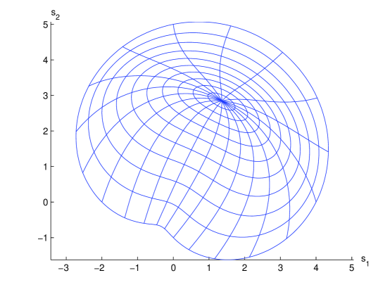
Figure 1: The region $\Omega$ associated with (46) and the mapping $\Phi$

We begin with planar examples, followed by some problems on regions $\Omega$ in $\mathbb{R}^{3}$. The examples will all be for the equation

$$\frac{\partial u\left(s,t\right)}{\partial t}=\Delta u\left(s,t\right)+f\left(s,t,u\left(s,t\right)\right),\quad\quad s\in\Omega,\quad t\geq 0.$$ (42)

To help in constructing our examples, we use

$$f\left(s,t,z\right) =f_{1}\left(s,t,z\right)+f_{2}\left(s,t\right).$$ (43)

We choose various $f_{1}$ to explore the effects of changes in the type of nonlinearity; and $f_{2}$ is then defined to make the equation (42) valid for any given $u$,

$$f_{2}\left(s,t\right) =\frac{\partial u\left(s,t\right)}{\partial t}-\left\{\Delta u\left(s,t\right)+f_{1}\left(s,t,u\left(s,t\right)\right)\right\},\>s\in\Omega,\quad t\geq 0.$$ (44)

In the reformulation (35), $A=I$ and thus

$$\widetilde{A}\left(x,t,z\right)=J\left(x\right)^{-1}J\left(x\right)^{-\text{T}}.$$ (45)

4.1 Planar examples

Begin with the region $\Omega$ whose boundary is a limacon. In particular, consider the boundary

$$\begin{array}[c]{l}\varphi\left(\theta\right)=\rho\left(\theta\right)\left(\cos\theta,\sin\theta\right),\\ \rho\left(\theta\right)=3+\cos\theta+2\sin\theta,\quad\quad 0\leq\theta\leq 2\pi.\end{array}$$ (46)

Using the methods of [6], we obtain a mapping $\Phi:\mathbb{B}_{2}\rightarrow\Omega$. Each component of $\Phi$ is a polynomial of degree 3. To illustrate the mapping we show the images in $\Omega$ of uniformly spaced circles and radial lines in $\mathbb{B}_{2}$; see Figure 1 and note that $\Omega$ is almost convex.

As a particular example for solving (42), let

$$f_{1}\left(s,t,z\right) =e^{-z}\cos\left(\pi t\right),\vskip 6.0pt plus 2.0pt minus 2.0pt$$ (47)

$$u\left(s,t\right) =\left(1-x_{1}^{2}-x_{2}^{2}\right)\cos\left(t+0.05\pi s_{1}s_{2}\right)$$ (48)

with $s=\Phi\left(x\right)$.  For the numerical integration in (37), $q=2n$ was chosen, where $n+2$ is the degree of the approximation $\widetilde{u}_{n}$. This choice of $q$ has always been more than adequate, and a smaller choice would often have sufficed.

To have a time interval of reasonable length, the problem was solved over $0\leq t\leq 20$, although something longer could have been chosen as well. The error was checked at 801 points of $\Omega$, chosen as the images under $\Phi$ of 801 points distributed over $\mathbb{B}_{2}$. The graph of $u_{12}\left(\cdot,20\right)$ is given in Figure 2, and the associated error is given in Figure 3; in addition, $\left\|u\left(\cdot,20\right)-u_{12}\left(\cdot,20\right)\right\|_{\infty}\doteq 1.94E-4$. Figure 4 shows the error norm $\left\|u\left(\cdot,t\right)-u_{12}\left(\cdot,t\right)\right\|_{\infty}$ for 200 evenly spaced values of $t$ in $\left[0,20\right]$. There is an oscillatory behaviour which is in keeping with that of the solution $u$. To illustrate the spectral rate of convergence of the method, Figure 5 gives the error as the degree $n$ varies from $6$ to $20$. The linear behaviour of this semi-log graph implies an exponential rate of convergence of $u_{n}$ to $u$ as a function of $n$.

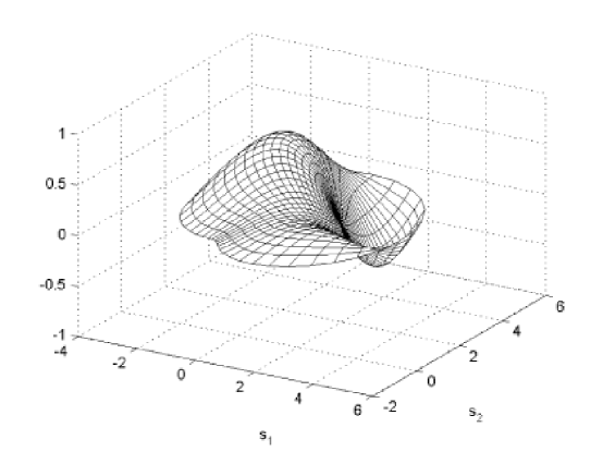
Figure 2: The approximating solution $u_{12}\left(s,20\right)$ for the true solution $u\left(s,20\right)$ of (48) over $\Omega$

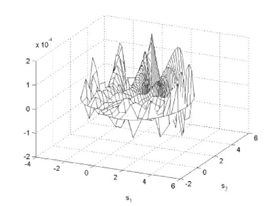
Figure 3: The error in the approximating solution $u_{12}\left(s,20\right)$ for the true solution $u\left(s,20\right)$ of (48) over $\Omega$

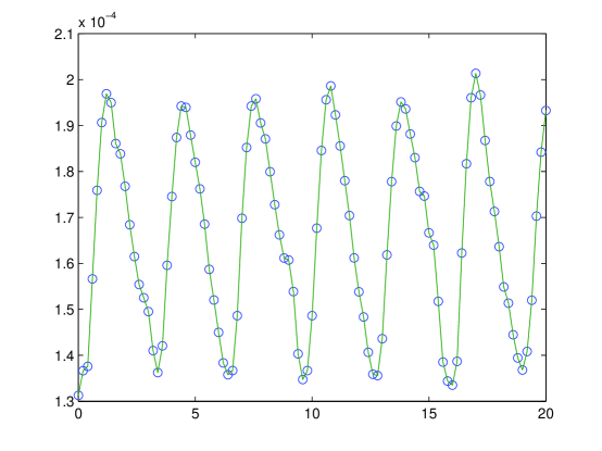
Figure 4: The error $\left\|u\left(\cdot,t\right)-u_{12}\left(\cdot,t\right)\right\|_{\infty}$ for the true solution $u\left(s,t\right)$ of (48)

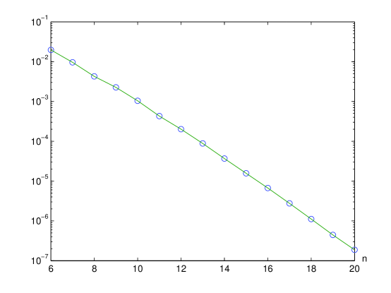
Figure 5: $n$ vs. $\max\limits_{0\leq t\leq 20}\left\|u\left(\cdot,t\right)-u_{n}\left(\cdot,t\right)\right\|_{\infty}$

An important aspect on which we have not yet commented is the conditioning of the matrices in the system (27). In our use of the Matlab program ode15s, we have written (27) in the form

$$\mathsf{a}_{N}^{{}^{\prime}}\left(t\right)=G_{n}^{-1}B_{n}\left(t,u_{n}\right)\mathsf{a}_{N}\left(t\right)+G_{n}^{-1}\boldsymbol{f}_{N}\left(t,u_{n}\right),$$ (49)

The matrix $G_{n}^{-1}B_{n}\left(t,u_{n}\right)$ is the Jacobian matrix for this system.  Investigating experimentally,

$$\operatorname*{cond}\left(G_{n}^{-1}B_{n}\right)=\mathcal{O}\left(N_{n}^{2}\right)$$ (50)

where $N_{n}$ is the number of equations in (49). As support for this assertion, Figure 6 shows the graph of $\log\left(N_{n}^{2}\right)$ vs. $\log\left(\operatorname*{cond}\left(G_{n}^{-1}B_{n}\right)\right)$. There is a clear linear behaviour and the slope is approximately 1, thus supporting (50). When $\Omega$ is the unit disk, and $\Phi=I$, the result (50) is still valid experimentally.

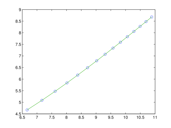
Figure 6: $\log\left(N_{n}^{2}\right)$ vs. $\log\left(\operatorname*{cond}\left(G_{n}^{-1}B_{n}\right)\right)$ for limacon region

As a second example, one for which $\Omega$ is much more nonconvex (although still star-like), consider the region $\Omega$ with the given boundary function

$$\begin{array}[c]{l}\varphi\left(\theta\right)=\rho\left(\theta\right)\left(\cos\theta,\sin\theta\right),\\ \rho\left(\theta\right)=5+\sin\theta+\sin 3\theta-\cos 5\theta,\quad\quad 0\leq\theta\leq 2\pi.\end{array}$$ (51)

As before, an extension $\Phi$ to $\mathbb{B}_{2}$ is constructed using the methods of [6]. The mapping $\Phi$ is a polynomial of degree 7 in each component; and the images in $\Omega$ of uniformly spaced circles and radial lines in $\mathbb{B}_{2}\,\$are shown in Figure 7.

Again, use the function $f_{1}$ of (47) and the solution $u$ of (48). The solution $u_{20}\left(\cdot,20\right)$ is shown in Figure 8 over this new region, and $\left\|u\left(\cdot,20\right)-u_{20}\left(\cdot,20\right)\right\|_{\infty}$ $\doteq 0.00136$. Figure 9 shows the error in $u_{20}\left(\cdot,t\right)$ over time, and Figure 10 shows how the error in $u_{n}$ varies with the degree $n$. The latter again indicates a spectral order of convergence, although slower than that shown in Figure 5. The condition numbers still satisfy the empirical estimate of (50).

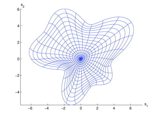
Figure 7: The region $\Omega$ associated with (51) and the mapping $\Phi$

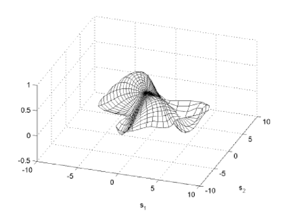
Figure 8: The approximating solution $u_{20}\left(s,20\right)$ for the true solution $u\left(s,20\right)$ of (48) over the $\Omega$ of Figure 7

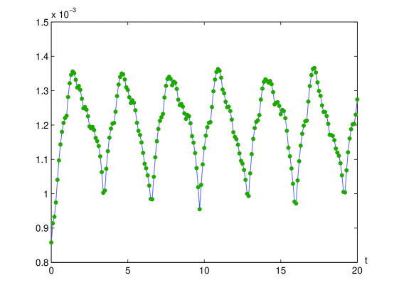
Figure 9: The error $\left\|u\left(\cdot,t\right)-u_{20}\left(\cdot,t\right)\right\|_{\infty}$ for the true solution $u\left(s,t\right)$ of (48) over the $\Omega$ of Figure 7

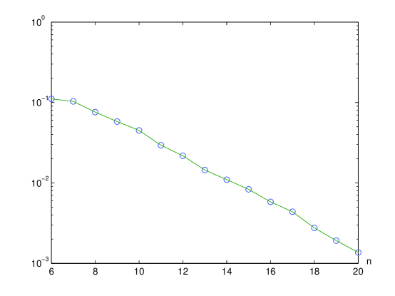
Figure 10: $n$ vs. $\max\limits_{0\leq t\leq 20}\left\|u\left(\cdot,t\right)-u_{n}\left(\cdot,t\right)\right\|_{\infty}$ for the $\Omega$ of Figure 7

4.2 A three-dimensional example

Here we will study one domain $\Omega$ which we investigated already in a previous article for the purpose of analyzing the spectral method for Dirichlet problems; see [2]. The domain has the advantage that the transformation $\Phi$ is known throughout $\mathbb{B}_{3}$ and even the inverse transformation $\Psi$ is known explicitly. The knowledge of $\Psi$ is not necessary for the use of the spectral method but makes the construction of an explicit solution easier. The mapping $\Phi:\overline{\mathbb{B}}_{3}\mapsto\overline{\Omega}$, $(s_{1},s_{2},s_{3})=\Phi(x_{1},x_{2},x_{3})$ is given by

$$\begin{array}[c]{rcl}s_{1}&=&x_{1}-x_{2}+ax_{1}^{2}\\ s_{2}&=&x_{1}+x_{2}\\ s_{3}&=&2x_{3}+bx_{3}^{2}\end{array}$$ (52)

where $0<a,b<1$ are two parameters.

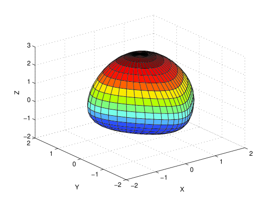
Figure 11: The surface of $\Omega$ with parameters $a=0.7$ and $b=0.9$; see (52)

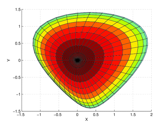
Figure 12: The surface of $\Omega$, see (52), seen from the $z$-axis

Figures 11, 12 show an example of the surface of $\Omega$ from two different angles. The inverse $\Psi:\overline{\Omega}\mapsto\overline{\mathbb{B}}_{3}$ is given by

$$x_{1} =\frac{1}{a}\left[-1+\sqrt{1+a(s_{1}+s_{2})}\right]$$

$$x_{2} =\frac{1}{a}\left[as_{2}+1-\sqrt{1+a(s_{1}+s_{2})}\right]$$

$$x_{3} =\frac{1}{b}\left[-1+\sqrt{1+bs_{3}}\right]$$

Furthermore the Jacobian for $\Phi$ is given by

$$J(x)=\left(\begin{array}[c]{ccc}1+2ax_{1}&-1&0\\ 1&1&0\\ 0&0&2+2bx_{3}\end{array}\right)$$

with determinant

$$\det(J(x))=4(1+ax_{1})(1+bx_{3}).$$

This allows us also to calculate $\widetilde{A}$, see (45), directly

$$\widetilde{A}(x)=\left(\begin{array}[c]{ccc}\dfrac{1}{2(1+ax_{1})^{2}}&\dfrac{ax_{1}}{2(1+ax_{1})^{2}}&0\\ \dfrac{ax_{1}}{2(1+ax_{1})^{2}}&\dfrac{1+ax_{1}+2a^{2}x_{1}^{2}}{2(1+ax_{1})^{2}}&0\\ 0&0&\dfrac{1}{4(1+bx_{3})^{2}}\end{array}\right)$$

Again we use the spectral method to solve (42) where $f$ is given by (43) and (44). As a particular example for solving (42), let

$$f_{1}(s,t,z) =e^{-z}\cos(\pi t),$$

$$u(s,t) =(1-x_{1}^{2}-x_{2}^{2}-x_{3}^{2})\cos(t+0.05\pi s_{1}s_{2}s_{3})$$ (53)

where $(x_{1},x_{2},x_{3})=\Psi(s_{1},s_{2},s_{3})$ with $a=0.7$ and $b=0.9$. Numerical results are given in Figures 13, 14. Figure 15 seems to indicate that the relation (50) for the condition number of the Jacobian $G_{n}^{-1}B_{n}$ is also valid in the three dimensional case.

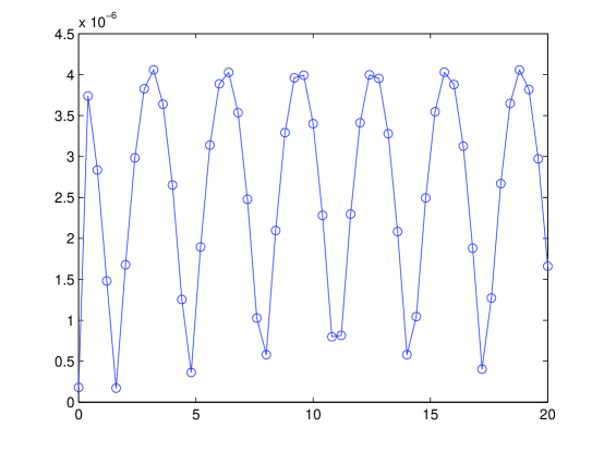
Figure 13: The error $\left\|u\left(\cdot,t\right)-u_{12}\left(\cdot,t\right)\right\|_{\infty}$ for the true solution $u\left(s,t\right)$ of (53) over the $\Omega$ of Figure 11

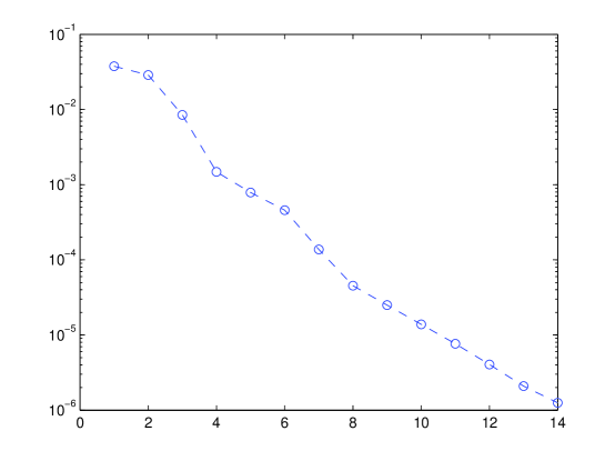
Figure 14: $n$ vs. $\max\limits_{0\leq t\leq 20}\left\|u\left(\cdot,t\right)-u_{n}\left(\cdot,t\right)\right\|_{\infty}$ over the $\Omega$ of Figure 11

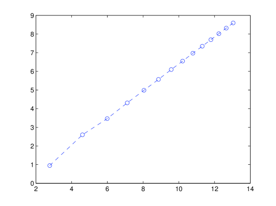
Figure 15: $\log\left(N_{n}^{2}\right)$ vs. $\log\left(\operatorname*{cond}\left(G_{n}^{-1}B_{n}\right)\right)$ for the $\Omega$ of Figure 11

References

- [1] M. Abramowitz, I.A. Stegun. Handbook of Mathematical Functions, Dover Publications, Inc., New York, 1965.
- [2] K. Atkinson, D. Chien, and O. Hansen. A spectral method for elliptic equations: The Dirichlet problem, Advances in Computational Mathematics, 33 (2010), pp. 169-189.
- [3] K. Atkinson, W. Han, and D. Stewart. Numerical Solution of Ordinary Differential Equations, John Wiley Pub., 2009.
- [4] K. Atkinson and O. Hansen. Solving the nonlinear Poisson equation on the unit disk, J. Integral Eqns. & Applic. 17 (2005), pp. 223-241.
- [5] K. Atkinson and O. Hansen. A spectral method for the eigenvalue problem for elliptic equations, Electronic Transactions on Numerical Analysis 37 (2010), pp. 386-412.
- [6] K. Atkinson and O. Hansen. Creating domain mappings, Electronic Transactions on Numerical Analysis, to appear. Preliminary version available at http://arxiv.org/abs/1106.3338.
- [7] K. Atkinson, O. Hansen, and D. Chien. A spectral method for elliptic equations: The Neumann problem, Advances in Computational Mathematics 34 (2011), pp. 295-317.
- [8] K. Atkinson and W. Han. Theoretical Numerical Analysis: A Functional Analysis Framework, 3 ed., Springer-Verlag, New York, 2009.
- [9] K. Atkinson and W. Han. An Introduction to Spherical Harmonics and Approximations on the Unit Sphere, Springer-Verlag, New York, 2012.
- [10] J. Boyd. Chebyshev and Fourier Spectral Methods, 2 ed., Dover Pub., New York, 2000.
- [11] C. Canuto, A. Quarteroni, My. Hussaini, and T. Zang. Spectral Methods in Fluid Mechanics, Springer-Verlag, 1988.
- [12] C. Canuto, A. Quarteroni, My. Hussaini, and T. Zang. Spectral Methods - Fundamentals in Single Domains, Springer-Verlag, 2006.
- [13] J. Douglas and T. Dupont. Galerkin methods for parabolic equations, SIAM J. Num. Anal. 7 (1970), 575-626.
- [14] C. Dunkl and Y. Xu. Orthogonal Polynomials of Several Variables, Cambridge Univ. Press, Cambridge, 2001.
- [15] W. Gautschi. Orthogonal Polynomials, Oxford University Press, Oxford, 2004.
- [16] D. Gottlieb and S. Orszag. Numerical Analysis of Spectral Methods: Theory and Applications, SIAM Pub., 1977.
- [17] Ben-Yu Guo. Spectral Methods and Their Applications, World Scientific, 1998.
- [18] E. W. Hobson. The Theory of Spherical and Ellipsoidal Harmonics, Chelsea Publishing, New York, 1965.
- [19] B. Logan and L. Shepp. Optimal reconstruction of a function from its projections, Duke Mathematical Journal 42, (1975), 645–659.
- [20] D. Ragozin. Constructive polynomial approximation on spheres and projective spaces, Trans. Amer. Math. Soc. 162 (1971), 157-170.
- [21] L. Shampine, I. Gladwell, and S. Thompson. Solving ODEs with MATLAB, Cambridge University Press, 2003.
- [22] J. Shen and T. Tang. Spectral and High-Order Methods with Applications, Science Press, Beijing, 2006.
- [23] J. Shen, T. Tang, and L. Wang. Spectral Methods: Algorithms, Analysis and Applications, Springer-Verlag, 2011.
- [24] A. Stroud. Approximate Calculation of Multiple Integrals, Prentice-Hall, Inc., Englewood Cliffs, N.J., 1971.
- [25] Yuan Xu. Lecture notes on orthogonal polynomials of several variables, in Advances in the Theory of Special Functions and Orthogonal Polynomials, Nova Science Publishers, 2004, 135-188.
- [26] E. Zeidler. Nonlinear Functional Analysis and Its Applications: II/B, Springer-Verlag, Berlin, 1990.
- [27] S. Zhang and J. Jin. Computation of Special Functions, John Wiley & Sons, New York, 1996.