Soliton Magnetization Dynamics in Spin-Orbit Coupled Bose-Einstein Condensates

Abstract

Ring-trapped Bose-Einstein condensates subject to spin-orbit coupling support localized dark soliton excitations that show periodic density dynamics in real space. In addition to the density feature, solitons also carry a localized pseudo-spin magnetization that exhibits a rich and tunable dynamics. Analytic results for Rashba-type spin-orbit coupling and spin-invariant interactions predict a conserved magnitude and precessional motion for the soliton magnetization that allows for the simulation of spin-related geometric phases recently seen in electronic transport measurements.

The recent realization of artificial light-induced gauge potentials for neutral atoms Lin et al. (2009) has added a powerful new instrument to the atomic-physics simulation toolkit Dalibard et al. (2011). In particular, possibilities to induce Zeeman-like and spin-orbit-type couplings in (pseudo-)spinor atom gases Lin et al. (2011) render them ideal laboratories to investigate the intriguing interplay of spin dynamics and quantum confinement that has been the hallmark of semiconductor spintronics Awschalom et al. (2002); Zutić et al. (2004). At the same time, the unique aspects of Bose-Einstein-condensed atom gases Pitaevskii and Stringari (2003) associated, e.g., with their intrinsically nonlinear dynamics, promise to give rise to novel behavior under the influence of synthetic spin-orbit couplings Stanescu et al. (2008); Merkl et al. (2010a); Wang et al. (2010); Ho and Zhang (2011); Wu et al. (2011); Yip (2011); Sinha et al. (2011); Hu et al. (2012); Zhang et al. (2012).

One of the special properties resulting from nonlinearity in Bose-Einstein condensates (BECs) is the existence of solitary-wave excitations Carretero-Gonzáez et al. (2008). Basic types of these are distinguished by the shape of their localized density feature: dark (gray) solitons are associated with a full (partial) depletion of a uniform condensate density in a finite region of space, whereas bright solitons are localized density waves on an empty background. A further characteristic associated with solitons is the phase gradient of the condensate order parameter centered at the position of the density feature. In multi-component systems, the dynamics of soliton excitations is found to be enriched by the additional degrees of freedom Manakov (1973); Sheppard and Kivshar (1997); Öhberg and Santos (2001); Smyrnakis et al. (2010).

Figure 1: Time evolution of a gray-bright soliton’s magnetization in a ring-trapped BEC with Rashba spin-orbit coupling. During a full cycle of the soliton’s motion on the ring, the magnetization vector follows a trajectory on the surface of a sphere. The magnetization vectors at the beginning and the end of a cycle (indicated by arrows) differ by an angle $\vartheta$ that is related to a spin-related geometric phase. Soliton parameters (see text): $v_{\text{s}}/c=0.5$, $\tan\eta=2$, $g=100$, $\kappa=-0.01$.

We have studied solitons in ring-trapped pseudo-spin-$1/2$ condensates with spin-invariant repulsive atom-atom interactions subject to a Rashba-type Rashba (1960); Bychkov and Rashba (1984) spin-orbit coupling and find that they exhibit a third feature: a pseudo-magnetization vector with conserved magnitude and rich dynamics that unfolds in tandem with the soliton’s periodic propagation in real space. Figure 1 shows an example and also illustrates the interesting fact that the magnetization directions at the beginning and the end of a full cycle of the soliton’s motion are generally not parallel. The appearance of such a geometric phase Shapere and Wilczek (1989) and the precessional time evolution of the solitonic magnetization is reminiscent of the spin dynamics of electrons traversing a mesoscopic semiconductor ring Loss et al. (1990); Aronov and Lyanda-Geller (1993); Splettstoesser et al. (2003); Frustaglia and Richter (2004); Nagasawa et al. (2012).

In the following, we consider several soliton configurations and obtain analytical results for their density and magnetization profiles as well as the magnetization dynamics associated with their motion. We start by introducing the basic theoretical description of our system of interest. Using the basis of a spatially varying local spin frame Splettstoesser et al. (2003) for the condensate spinor, the nonlinear Gross-Pitaevskii equation Pitaevskii and Stringari (2003) for the spin-orbit-coupled ring BEC turns out to be of Manakov-type Manakov (1973), making it possible to apply standard methods Sheppard and Kivshar (1997); Smyrnakis et al. (2010) to find solitary-wave solutions. Accounting for the presence of spin-orbit coupling adds an important twist: Spinors have to satisfy non-standard boundary conditions, which introduce background-density flows in the local spin frame that contribute to the nontrivial magnetization dynamics exhibited by the moving solitons in the lab frame.

We consider a two-component BEC trapped in the $xy$ plane and confined to a ring of radius $R$. The atoms are assumed to be in the lowest quasi-onedimensional subband  and subject to a spin-orbit coupling of the familiar Rashba form Rashba (1960); Bychkov and Rashba (1984) $\alpha_{\text{R}}\left[\sigma_{x}(-i\partial_{y})-\sigma_{y}(-i\partial_{x})\right]$ as well as a spin-rotationally invariant contact interaction. (Here $\sigma_{x,y,z}$ are the spin-1/2 Pauli matrices.) The energy functional of such a system Merkl et al. (2010b) is given by $E[\Psi]=\int d\varphi\,\,\Psi^{{\dagger}}\,({\mathcal{H}}-\mu)\,\Psi$, where $\varphi$ is the azimuthal angle, $\mu$ the chemical potential, $\Psi=(\psi_{\uparrow},\psi_{\downarrow})^{T}$ the two-component (pseudo-spin-$1/2$) spinor order parameter in the representation where the ($z$) direction perpendicular to the ring’s plane is the spin-quantization axis, and

$${\mathcal{H}} = E_{0}\bigg{[}-\partial_{\varphi}^{2}+\frac{g}{2}\,\Psi^{\dagger}\Psi$$ (1)

$$\hskip 14.22636pt+\tan\eta\left(\sigma_{+}\mathrm{e}^{-i\varphi}+\sigma_{-}\mathrm{e}^{i\varphi}\right)\left(-i\partial_{\varphi}+\frac{\sigma_{z}}{2}\right)\bigg{]}.$$

We use $\sigma_{\pm}\equiv(\sigma_{x}\pm i\sigma_{y})/2$ to denote raising and lowering operators for spin-1/2 components, $E_{0}=\hbar^{2}/(2MR^{2})$ is the energy scale for quantum confinement of atoms with mass $M$ in a ring of radius $R$, $E_{0}g$ is the two-body contact-interaction strength, and $\tan\eta=2MR\,\alpha_{\text{R}}/\hbar^{2}$ is a dimensionless measure of the spin-orbit coupling.

The effect of Rashba spin-orbit coupling in a ring geometry can be elucidated by performing a suitable SU(2) transformation. Defining $\Psi={\mathcal{U}}\,\chi$ and ${\mathcal{H}}_{\text{loc}}={\mathcal{U}}^{-1}\mathcal{H}\,{\mathcal{U}}$, with ${\mathcal{U}}=\mathrm{e}^{-i\varphi\sigma_{z}/2}\,\mathrm{e}^{i{\eta}\sigma_{y}/2}\,\mathrm{e}^{i\varphi\sigma_{z}/(2\cos\eta)}$, we find

$${\mathcal{H}}_{\text{loc}}=E_{0}\left[-\partial_{\varphi}^{2}-\frac{(\tan\eta)^{2}}{4}+\frac{g}{2}\,\chi^{\dagger}\chi\right]\quad.$$ (2)

The transformation ${\mathcal{U}}^{-1}$ amounts to a $\varphi$-dependent rotation of the pseudo-spin quantization axis Splettstoesser et al. (2003), followed by a spin-dependent gauge transformation. We will refer to the original representation where the spin-quantization axis coincides with the axis of the ring as the lab frame, whereas the representation in which the Hamiltonian of the system is diagonal in pseudo-spin space [i.e., given by ${\mathcal{H}}_{\text{loc}}$ of Eq. (2)] will be the local spin frame Splettstoesser et al. (2003). Note that the spinors $\Psi$ in the lab frame are periodic functions of $\varphi$, whereas the spinors $\chi=(\chi_{+},\chi_{-})^{T}$ from the local spin frame have to satisfy the boundary conditions $\chi_{\pm}(\varphi)=\chi_{\pm}(\varphi+2\pi)e^{\pm i{\mathcal{A}}}$ with a spin dependent phase twist originating from the spin-orbit coupling, where

$${\mathcal{A}}=\pi\left(\frac{1}{\cos\eta}-1\right)\quad.$$ (3)

Knowledge of the local-spin-frame spinors enables the calculation of expectation values for any observables accessible to measurement in the lab frame. The total density $n=|\psi_{\uparrow}|^{2}+|\psi_{\downarrow}|^{2}\equiv|\chi_{+}|^{2}+|\chi_{-}|^{2}$ is obviously the same irrespective of which representation is chosen in spin space. The pseudo-spin-1/2 projections in the lab frame correspond to definite atomic states, hence their density profiles $n_{\uparrow(\downarrow)}=\Psi^{\dagger}([1+(-)\sigma_{z}]/2)\Psi$ are of interest. In addition, we will consider the magnetization-density vector ${\bm{\mathrm{s}}}=\Psi^{{\dagger}}{\bm{\mathrm{\sigma}}}\,\Psi$ in the lab frame, with ${\bm{\mathrm{\sigma}}}=(\sigma_{x},\sigma_{y},\sigma_{z})$ being the vector of Pauli matrices.

We analyze the properties of localized excitations in spin-orbit-coupled ring-trapped BEC based on the time-dependent Gross-Pitaevskii equation Pitaevskii and Stringari (2003) $\delta E[\chi]/\delta\chi_{\sigma}^{\ast}=i\hbar\,\partial\chi_{\sigma}/\partial t$. After rescaling to use the dimensionless time variable $\tau=tE_{0}/\hbar$, it has the form

$$i\,\frac{\partial\chi_{\sigma}}{\partial\tau}=\left[-\partial^{2}_{\varphi}+g\,\left(\left|\chi_{+}\right|^{2}+\left|\chi_{-}\right|^{2}-n_{0}\right)\right]\chi_{\sigma}$$ (4)

for the two components of the spinor $\chi=(\chi_{+},\chi_{-})^{T}$, where $n_{0}=[\mu+(\tan\eta)^{2}/4]/(gE_{0})$ is the uniform (background) density consistent with the chemical potential $\mu$. While the spin-orbit coupling has formally disappeared from the nonlinear equation (4), it is still implicitly present via the boundary conditions that the individual components $\chi_{\pm}(\varphi,\tau)$ must satisfy.

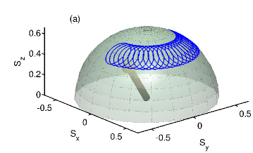
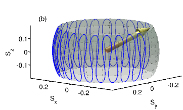
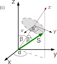
Figure 2: Magnetization dynamics of a gray-bright soliton [panel (a)] and a gray-gray soliton with zero background magnetization in the local spin frame [panel (b)]. Parameters used are $g=100$ ($100$), $\tan\eta=0.2$ ($0.5$), $v_{\text{s}}/c=0.5$ (0.2), and $\kappa=-0.5$ for the gray-bright (gray-gray) case. (c) Angles used to describe the two-step precessional motion of ${\bm{\mathrm{S}}}$. The angle $\alpha^{\prime}$ is measured with respect to an $x^{\prime}$ axis that is perpendicular to both the $z$ and $z^{\prime}$ axes.

We have obtained several soliton solutions of Eqs. (4) using established techniques Manakov (1973); Sheppard and Kivshar (1997); Smyrnakis et al. (2010) and implemented the appropriate boundary conditions. Before giving further details, we like to summarize a few general features. The soliton spinors in the local-spin-frame representation turn out to be of the form

$$\chi_{\sigma}^{(\text{s})}=\Upsilon^{(\text{s})}_{\sigma}(\varphi-v_{\text{s}}\tau)\,\mathrm{e}^{iv_{\text{b}\sigma}{\varphi}/2-iv_{\text{b}\sigma}^{2}\tau/4}\quad,$$ (5)

where $\Upsilon^{(\text{s})}_{\sigma}(\xi)$ are complex amplitude functions encoding the specific soliton-like density features, $v_{\text{s}}$ is the propagation speed of the soliton, and $v_{\text{b}\sigma}$ are background flow velocities of the individual spinor components that are necessary to implement the boundary conditions arising due to the presence of spin-orbit coupling. The density $n_{\uparrow(\downarrow)}^{\text{(s)}}$ and magnetization density ${\bm{\mathrm{s}}}^{\text{(s)}}$ exhibit spatially localized features. Subtracting ${\bm{\mathrm{s}}}^{\text{(s)}}$ from the magnetization density ${\bm{\mathrm{s}}}_{\text{b}}^{\text{(s)}}$ of the condensate background yields the magnetization density that is associated with the soliton excitation only. Its integral ${\bm{\mathrm{S}}}^{\text{(s)}}=\int d\varphi\,\,[{\bm{\mathrm{s}}}_{\text{b}}^{\text{(s)}}-{\bm{\mathrm{s}}}^{\text{(s)}}]$ is the vector of total soliton magnetization, which is an additional property of localized excitations in multi-component BECs. For soliton solutions of the form (5), ${\bm{\mathrm{S}}}^{\text{(s)}}$ has constant magnitude. Its temporal evolution is most conveniently described by a set of four angles as defined in Fig. 2(c). While the tilt angles $\beta$ and $\beta^{\prime}$ are time-independent, the angles $\alpha$ and $\alpha^{\prime}$ vary linearly in time, signifying the precession of ${\bm{\mathrm{S}}}^{\text{(s)}}$ around tilted $z^{\prime}$ axis with the universal result

$$\beta=\eta,\quad\alpha=v_{\text{s}}\tau+\pi.$$ (6)

The $z^{\prime}$ axis is tilted by the angle $\eta$ characterizing the spin-orbit coupling and it rotates around the $z$ axis with the same angular velocity $v_{\text{s}}$ that characterizes the soliton propagation. The second tilt angle $\beta^{\prime}$ is found to depend only on the soliton profile $\Upsilon_{\pm}(\varphi)$, while the precession frequency $d\alpha^{\prime}/d\tau$ has complicated dependences on the parameters of the soliton solutions. Figure 2 shows exemplary magnetization dynamics for gray-bright and gray-gray solitons. Interestingly, we find that the magnetization vector is usually not parallel to its initial direction after the soliton has completed a full cycle of its motion around the ring as, e.g. seen in figure 1. The angle $\vartheta$ between the magnetization directions at the start and the end of a cycle turns out to be finite only as a consequence of spin-orbit coupling, as it depends prominently on the phase ${\mathcal{A}}$ given in Eq. (3) that also governs spin-dependent interference in mesoscopic ring conductors Frustaglia and Richter (2004).

In order to find explicit soliton solutions, we introduce $\xi={\varphi}-u\tau$, where $u$ is a velocity parameter, and initially look for solutions of the form $\chi_{\sigma}(\varphi,\tau)=\sqrt{n_{\sigma}(\xi)}\,\mathrm{e}^{i\theta_{\sigma}(\xi)}$. This allows us to rewrite Eq. (4) in the form

$$-u\frac{\partial n_{\sigma}}{\partial\xi}+2\frac{\partial}{\partial\xi}\left(n_{\sigma}\frac{\partial\theta_{\sigma}}{\partial\xi}\right)=0\,,\qquad$$ (7a)

$$u\frac{\partial\theta_{\sigma}}{\partial\xi}+\frac{1}{\sqrt{n_{\sigma}}}\frac{\partial^{2}\sqrt{n_{\sigma}}}{\partial^{2}\xi}-\left(\frac{\partial\theta_{\sigma}}{\partial\xi}\right)^{2}-g(n-n_{0})=0\,,\qquad$$ (7b)

where $n=n_{+}+n_{-}$. Single component solutions for $\sigma=\tilde{\sigma}$ are easily found by integration of Eqs. (7) to yield $\chi_{\tilde{\sigma}}(\xi)\propto\Upsilon(\xi)$ and $\chi_{-\tilde{\sigma}}=0$, with the well-known dark soliton solution on the infinite line Pitaevskii and Stringari (2003)

$${\Upsilon(\xi)=\sqrt{n_{0}}\,\left[i\frac{u}{c}+\gamma_{u}\tanh\left(\gamma_{u}\,\frac{\xi}{\xi_{\text{D}}}\right)\right]\quad.}$$ (8)

Here $\gamma_{u}^{2}=1-u^{2}/c^{2}$, $c^{2}=2gn_{0}$, $1/\xi_{\text{D}}^{2}=gn_{0}/2$. The soliton profile (8) is appropriate for sufficiently strong nonlinearity, where $\xi_{D}/\gamma_{u}\ll 2\pi$ . However, $\Upsilon(\xi)$ does not satisfy the proper boundary condition since it has a phase step $\Delta\theta=-2\arccos(u/c)$. To compensate for the phase step and ensure the correct phase shift associated with the gauge transformation ${\mathcal{U}}$, we perform a Galilean transformation on (8), which yields

$$\chi^{\text{SC}}_{\tilde{\sigma}}({\varphi},\tau)=\Upsilon(\xi-v_{\text{b}}\tau)\,\mathrm{e}^{iv_{\text{b}}{\varphi}/2-iv_{\text{b}}^{2}\tau/4}\quad.$$ (9)

Here $v_{\text{b}}=-(\Delta\theta+{\tilde{\sigma}}{\cal A})/\pi$ is the background velocity imposed by the boundary condition. Thus the single-component soliton solution is of the form (5), with $\Upsilon^{\text{SC}}_{\tilde{\sigma}}=\Upsilon$ and $\Upsilon^{\text{SC}}_{-\tilde{\sigma}}=0$, and propagation speed $v_{\text{s}}=u+v_{\text{b}}$.

A straightforward calculation yields ${\bm{\mathrm{s}}}^{\text{SC}}=\tilde{\sigma}|\Upsilon(\varphi-v_{\text{s}}\tau)|^{2}(-\sin\eta\,\cos\varphi,-\sin\eta\,\sin\varphi,\cos\eta)^{T}$ for the magnetization density of the single-component soliton solution. In essence, the density depletion at the soliton’s position gives rise to a reduction of the magnetization density ${\bm{\mathrm{s}}}_{\text{b}}^{\text{SC}}=\tilde{\sigma}\,n_{0}(-\sin\eta\,\cos\varphi,-\sin\eta\,\sin\varphi,\cos\eta)^{T}$ associated with the background. Thus ${\bm{\mathrm{s}}}_{\text{b}}^{\text{SC}}-{\bm{\mathrm{s}}}^{\text{SC}}$ constitutes the magnetization density associated with the soliton itself, as it is the change in the background magnetization density due to the presence of the localized excitation. For the single-component soliton, this corresponds to a peak in magnetization density at the soliton’s position. The total magnetization vector is obtained by integrating that peak in real space, which yields ${\bm{\mathrm{S}}}^{\text{SC}}=\tilde{\sigma}(-\sin\eta\,\cos(v_{\text{s}}\tau),-\sin\eta\,\sin(v_{\text{s}}\tau),\cos\eta)^{T}$. This magnetization vector is precessing in a perfectly synchronized fashion with the soliton’s motion around the ring [cf. Fig. 2(c) with Eq. (6) and $\beta^{\prime}=0$], i.e., $\vartheta^{\text{SC}}=0$.

We now consider a solution of Eqs. (7) that is a gray-bright (GB) soliton in the local spin frame. We assume that the densities approach constant values $n_{+}\rightarrow n_{0+}$ (gray part) and $n_{-}\rightarrow 0$ (bright part) far away from the soliton’s position. To decouple Eq. (7b), we use the ansatz Smyrnakis et al. (2010) $n_{-}=\kappa(n_{+}-n_{0+})$ with $-1\leq\kappa\leq 0$. We apply a Galilean boost to both components to match the phase of the gray part only, hence they are of the form (5) with $\Upsilon^{\text{GB}}_{+}(\xi)$ given by $\Upsilon(\xi)$ from Eq. (8) but with rescaled $c^{2}=2gn_{0+}(1+\kappa)$, $1/\xi_{\text{D}}^{2}=gn_{0+}(1+\kappa)/2$, and

$$\Upsilon^{\text{GB}}_{-}(\xi)=\sqrt{-\kappa n_{0+}}\,\frac{\gamma_{u}\,\mathrm{e}^{iu\xi/2}}{\cosh(\gamma_{u}\xi/\xi_{\text{D}})}\quad.$$ (10)

Furthermore, $v_{\text{b}-}=v_{\text{b}+}$ and $v_{\text{s}}=u+v_{\text{b}+}$. Figure 3 shows the density profiles [panel (a)] and magnetization-density profile [panel (c)] associated with a GB soliton.

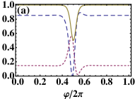
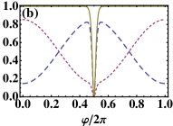
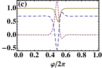
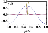
Figure 3: Lab-frame spin densities [(a),(b)] and $z$ component of the magnetization density [(c),(d)] for a stationary gray-bright soliton [(a),(c)] and a stationary gray-gray soliton [(b),(d)]. Panels (a) and (b) show the total density (solid yellow curve) and individual-spin (dashed blue $=$ $\uparrow$, dotted red $=$ $\downarrow$) densities normalized to the background-density value. In (c) and (d), the total density is plotted again for reference as the solid yellow curve, together with the magnetization profiles $s_{z}^{\text{(s)}}$ (dashed blue curve), and the magnetization density $s^{\text{(s)}}_{\text{b}\,z}-s^{\text{(s)}}_{z}$ associated with the soliton excitations only (dotted red curve). Parameters are $\tan\eta=1.0$, $g=100$, and (for the gray-bright soliton) $\kappa=-0.5$.

The vector ${\bm{\mathrm{S}}}^{\text{GB}}$ of total magnetization for a GB soliton precesses concomitantly with the soliton’s motion; cf. Fig. 2(c) with Eq. (6) and $\tan\beta^{\prime}=(\sqrt{-\kappa}u\pi)/[(1-\kappa)c\gamma_{u}]$, $\alpha^{\prime}=-v_{\text{s}}\tau(1+{\cal A}/\pi)$. Figures 1(a) and 2(a) show examples of possible time evolutions of the GB-soliton magnetization. The magnitude of the magnetization vector is found to be $S=2(1-\kappa)\xi_{D}\gamma_{u}/\cos\beta^{\prime}$. For a GB soliton, the magnetization vector turns out to be not aligned with its initial direction after completion of a full cycle of its motion around the ring. A straightforward calculation yields $\sin(\vartheta^{\text{GB}}/2)=\sin\beta^{\prime}\,\sin{\mathcal{A}}$. As $\beta^{\prime}$ is a known function of the soliton parameters, a measurement of $\vartheta^{\text{GB}}$ will yield the spin-related geometric phase ${\mathcal{A}}$.

The solutions representing gray-gray (GG) solitons in the local spin frame are obtained by Hirota’s method Sheppard and Kivshar (1997). The spinor components are of the form (5) with

$$\Upsilon_{\sigma}^{\text{GG}}(\xi)=\sqrt{n_{0\sigma}}\left[i\frac{u_{\sigma}}{c_{\sigma}}+\gamma_{u_{\sigma}}\tanh(a\xi)\right]\quad.$$ (11)

Here, $a^{2}=\gamma_{u_{+}}^{2}/\xi_{\text{D}+}^{2}+\gamma_{u_{-}}^{2}/\xi_{\text{D}-}^{2}$, $v_{\text{s}}=2au_{\sigma}/c_{\sigma}\gamma_{u_{\sigma}}+v_{\text{b}\sigma}$, $c_{\sigma}^{2}=2gn_{0\sigma}$, $1/\xi^{2}_{\text{D}\sigma}=gn_{0\sigma}/2$. The back-ground flows are given by $v_{\text{b}\sigma}=-(\Delta\theta_{\sigma}+\sigma{\cal A})/\pi$, where $\Delta\theta_{\sigma}=-2\arccos(u_{\sigma}/c_{\sigma})$. The independent parameters characterizing a GG soliton are the ratio $n_{0+}/n_{0-}$ (or, equivalently, the background magnetization in the local spin frame) and the speed $v_{\text{s}}$ of the soliton. All other parameters can be found by solving transcendental equations given just after Eq. (11). For simplicity, we consider the case of a GG soliton with zero background magnetization in the local spin frame (i.e., $n_{0+}=n_{0-}\equiv n_{0}/2$). Figure 3 shows results for spinor-density [panel (b)] and magnetization-density [panel (d)] profiles.

The time evolution of the magnetization vector associated with a moving GG soliton is characterized by the angles defined in Fig. 2(c) with Eq. (6), $\beta^{\prime}=\pi/2$, and $\alpha^{\prime}=\omega\tau+\pi/2$, where $\omega=-(v_{\text{b}+}-v_{\text{b}-})v_{\text{s}}/2+(v_{\text{b}+}^{2}-v_{\text{b}-}^{2})/4-(1+{\cal A}/\pi)v_{\text{s}}$. Figure 2(b) illustrates this dynamics which, for small $\eta$, corresponds to a slow rotation of the magnetization vector in the ring’s plane with superimposed fast small-amplitude oscillations in the normal direction. As in the case of the GB soliton, the magnetization vector does not evolve back to its initial direction after a period of the soliton’s ring revolution. The angle between magnetizations at the start and the end of the cycle is found to be $\vartheta^{\text{GG}}=2\pi|\omega|/v_{\text{s}}\rightarrow 2{\mathcal{A}}$ for ${\mathcal{A}}\ll 1$. Again, the dependence of $\vartheta^{\text{GG}}$ on ${\mathcal{A}}$ enables determination of the latter by measuring the former.

In conclusion, we have investigated the properties of soliton excitations in ring-trapped spin-orbit-coupled BECs. We find that a magnetization degree of freedom is generally associated with a soliton, and that the magnetization vector precesses around an axis that is rotating synchronously with the soliton’s orbital motion around the ring. The magnetization direction at the end of a cycle of revolution does not coincide with the initial direction for the gray-bright and gray-gray cases, making it possible to measure a spin-orbit-related geometric phase. Our work opens up new avenues for the realization and manipulation of magnetic soliton excitations in BECs. It also creates the opportunity to study spin-dependent interference and scattering effects that, until now, were only accessible in semiconductor nanostructures.

This work was supported by the Marsden fund (contract no. MAU0910) administered by the Royal Society of New Zealand.

References

- Lin et al. (2009) Y.-J. Lin, R. L. Compton, K. Jimenez-Garcia, J. V. Porto, and I. B. Spielman, Nature 462, 628 (2009).
- Dalibard et al. (2011) J. Dalibard, F. Gerbier, Juzeliūnas, and P. Öhberg, Rev. Mod. Phys. 83, 1523 (2011).
- Lin et al. (2011) Y.-J. Lin, K. Jimenez-Garcia, and I. B. Spielman, Nature (London) 471, 83 (2011).
- Awschalom et al. (2002) D. D. Awschalom, D. Loss, and N. Samarth, eds., Semiconductor Spintronics and Quantum Computation (Springer, Berlin, 2002).
- Zutić et al. (2004) I. Zutić, J. Fabian, and S. D. Sarma, Rev. Mod. Phys. 76, 323 (2004).
- Pitaevskii and Stringari (2003) L. Pitaevskii and S. Stringari, Bose-Einstein Condensation (Clarendon Press, Oxford, 2003).
- Stanescu et al. (2008) T. D. Stanescu, B. Anderson, and V. Galitski, Phys. Rev. A 78, 023616 (2008).
- Merkl et al. (2010a) M. Merkl, A. Jacob, F. E. Zimmer, P. Öhberg, and L. Santos, Phys. Rev. Lett. 104, 073603 (2010a).
- Wang et al. (2010) C. Wang, C. Gao, C.-M. Jian, and H. Zhai, Phys. Rev. Lett. 105, 160403 (2010).
- Ho and Zhang (2011) T.-L. Ho and S. Zhang, Phys. Rev. Lett. 107, 150403 (2011).
- Wu et al. (2011) C.-J. Wu, I. Mondragon-Shem, and X.-F. Zhou, Chin. Phys. Lett. 28, 097102 (2011).
- Yip (2011) S.-K. Yip, Phys. Rev. A 83, 043616 (2011).
- Sinha et al. (2011) S. Sinha, R. Nath, and L. Santos, Phys. Rev. Lett. 107, 270401 (2011).
- Hu et al. (2012) H. Hu, B. Ramachandhran, H. Pu, and X.-J. Liu, Phys. Rev. Lett. 108, 010402 (2012).
- Zhang et al. (2012) Y. Zhang, L. Mao, and C. Zhang, Phys. Rev. Lett. 108, 035302 (2012).
- Carretero-Gonzáez et al. (2008) R. Carretero-Gonzáez, D. J. Frantzeskakis, and P. G. Kevrekidis, Nonlinearity 21, R139 (2008).
- Manakov (1973) S. V. Manakov, Zh. Eksp. Teor. Fiz. 65, 505 (1973), [Sov. Phys. JETP 38, 248 (1974)].
- Sheppard and Kivshar (1997) A. P. Sheppard and Y. S. Kivshar, Phys. Rev. E 55, 4773 (1997).
- Öhberg and Santos (2001) P. Öhberg and L. Santos, Phys. Rev. Lett. 86, 2918 (2001).
- Smyrnakis et al. (2010) J. Smyrnakis, M. Magiropoulos, G. M. Kavoulakis, and A. D. Jackson, Phys. Rev. A 81, 063601 (2010).
- Rashba (1960) E. I. Rashba, Fiz. Tverd. Tela (Leningrad) 2, 1224 (1960), [Sov. Phys. Solid State 2, 1109 (1960)].
- Bychkov and Rashba (1984) Y. A. Bychkov and E. I. Rashba, J. Phys. C 17, 6039 (1984).
- Shapere and Wilczek (1989) A. Shapere and F. Wilczek, eds., Geometric Phases in Physics (World Scientific, Singapore, 1989).
- Loss et al. (1990) D. Loss, P. Goldbart, and A. V. Balatsky, Phys. Rev. Lett. 65, 1655 (1990).
- Aronov and Lyanda-Geller (1993) A. G. Aronov and Y. B. Lyanda-Geller, Phys. Rev. Lett. 70, 343 (1993).
- Splettstoesser et al. (2003) J. Splettstoesser, M. Governale, and U. Zülicke, Phys. Rev. B 68, 165341 (2003).
- Frustaglia and Richter (2004) D. Frustaglia and K. Richter, Phys. Rev. B 69, 235310 (2004).
- Nagasawa et al. (2012) F. Nagasawa, J. Takagi, Y. Kunihashi, M. Kohda, and J. Nitta, Phys. Rev. Lett. 108, 086801 (2012).
- Note (1) This limitation is not crucial, as finite-width effects and higher subbands could be treated straightforwardly.
- Merkl et al. (2010b) M. Merkl, G. Juzeliūnas, and P. Öhberg, Eur. Phys. J. D 59, 257 (2010b).
- Note (2) Otherwise periodic solutions involving elliptic functions have to be used. See, e.g., L. D. Carr, C. W. Clark, and W. P. Reinhardt, Phys. Rev. A 62, 063610 (2000).