Frustrated quantum Ising spins simulated
by spinless bosons in a tilted lattice:
from a quantum liquid to antiferromagnetic order

Abstract

We study spinless bosons in a decorated square lattice with a near-diagonal tilt. The resonant subspace of the tilted Mott insulator is described by an effective Hamiltonian of frustrated quantum Ising spins on a non-bipartite lattice. This generalizes an earlier proposal for the unfrustrated quantum Ising model in one dimension which was realized in a recent experiment on ultracold ⁸⁷Rb atoms in an optical lattice. Very close to diagonal tilt, we find a quantum liquid state which is continuously connected to the paramagnet. Frustration can be reduced by increasing the tilt angle away from the diagonal, and the system undergoes a transition to an antiferromagnetically ordered state. Using quantum Monte Carlo simulations and exact diagonalization, we find that for realistic system sizes the antiferromagnetic order appears to be quasi-one-dimensional; however, in the thermodynamic limit the order is two-dimensional.

I Introduction

Recent experimental progress in the field of ultracold atomic gases has made it possible to study quantum many-body physics in a controllable and clean setting. This makes cold atoms in optical lattices candidates for analog quantum simulators of real materials PhysRevLett.81.3108 ; RevModPhys.80.885 ; Bloch2012 ; Cirac2012 . Since the observation of a quantum phase transition from a superfluid state to an interaction driven insulating stateGreiner2002 , there has been much effort to simulate other correlated quantum phases, such as magnetic phases. Many proposals suggest using an internal degree of freedom of the atoms to simulate a spin degree of freedom1367-2630-5-1-113 ; PhysRevLett.90.100401 ; PhysRevA.84.031603 . Virtual hopping processes then lead to an effective magnetic interaction called superexchange AssaBook ; Trotzky18012008 . The energy scale of those processes is still low compared to experimentally reachable temperatures, and so magnetic long range order has not yet been observed.

An important milestone was recently reached taking a surprising new route: an equilibrium quantum phase transition of an antiferromagnetic spin chain was simulated using spinless bosons in a non-equilibrium situation. Following the theoretical proposal of Refs. SachdevMI, and PhysRevB.69.075106, , Simon et al.GreinerIsing examined a one-dimensional array of ⁸⁷Rb atoms in an optical lattice; an additional potential gradient (‘tilt’) drove the transition from the Mott insulating state to a state with density wave order. This happened in a metastable state, which is not the ground state of the full bosonic hamiltonian. However, the dynamics of the tilted lattice was confined to a resonantly connected effective subspace, which has an energy bounded from below, and so a mapping to an antiferromagnetic Ising model in a transverse and longitudinal field is possible.SachdevMI Changing the tilt magnitude corresponds to changing the strength of the longitudinal field, and this takes the systems through an Ising quantum phase transition, which was observed using single site resolutionsbakrgreiner2 ; Sherson2010 ; Gemelke2009 ; Gericke2008 ; Nelson2007 . The dynamics of the one-dimensional system has also been studied theoretically PhysRevA.69.053616 ; 1ddyn1 ; 1ddyn2 .

In Ref. PielawaTiltMI, , we have shown that a variety of correlated phases are possible in tilted two dimensional lattices. A mapping to a spin model is in general not possible in two dimensions. In this paper we focus on a lattice- and tilt configuration where a spin mapping is possible also in two dimension: a diagonally tilted decorated square lattice of bosons leads to a spin model on a non-bipartite lattice, the “octagon-square-cross lattice” (see Figure 1).

Figure 1: Decorated square lattice in a near-diagonal tilt: a) shows the physical lattice for the bosons. The spins reside on the links, which form the lattice shown in b). The effective resonant subspace of the boson model of the decorated square lattice (a) maps to an antiferromagnet on the octagon-square-cross lattice (b) in a strong longitudinal and in a transverse magnetic field. If the tilt is not exactly diagonal, then spins on horizontal lines experience a different longitudinal field than spins on vertical lines. The spin lattice is not bipartite, and in this sense the antiferromagnet is frustrated.

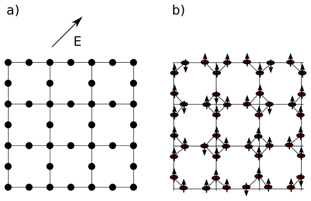
We start from the Mott insulator with a filling factor of one atom per lattice site, and assume that effective three-body interaction are important, such that triply occupied sites are not allowed. It has been shownPielawaTiltMI that in this system, three-body interactions have important qualitative effects; in particular, if three-body interaction are negligible, then the system maps to a quantum dimer model on a square lattice, as discussed in Ref. PielawaTiltMI, .

When the potential drop per lattice site is comparable to the on-site repulsion, then the only processes allowed in the resonant subspace are creations of ‘dipoles’ along the links of the lattice. A dipole is created when a boson follows the tilt direction and moves onto a neighboring site, which already contains one boson. This process costs the on-site repulsion energy $U$ and gains potential energy $E$. In the parameter regime $\left|U-E\right|\ll U,E$ all other processes are off-resonant.SachdevMI

Due to conservation of energy any lattice site can be part of no more than one dipole. We can map the Hamiltonian of the resonant subspace to a spin model by associating a spin state to each link: spin up if no dipole has been created on that link, and spin down if a dipole has been created on that link. The hard constraint forbidding overlapping dipoles translates to a strong antiferromagnetic interaction in a strong longitudinal field, and so we obtain an Ising antiferromagnet.

As this lattice is not bipartite, antiferromagnetic order is not possible, even for a weak longitudinal field (where the antiferromagnetic interaction dominates over the magnetic field). In this sense the Ising spin model on this lattice is geometrically frustrated.

Let us first briefly reviewPielawaTiltMI the case of a diagonal tilt. The parent Mott insulator remains stable to a weak tilt. In the other limit, the strongly tilted case, the system wants to maximize the number of dipoles. Due to the nearest-neighbor exclusion constraint, and due to the lattice geometry, there can be no more than one dipole per unit cell. The lattice has four links per unit cell, and so there is a lot of room for the dipoles to fluctuate. Quantum fluctuations then create a unique and gapped ground state: an equal amplitude superposition of all classically allowed dipole coverings PielawaTiltMI . This disordered quantum liquid state is continuously connected to the parent Mott insulator; it is part of the same phase, as shown in the phase diagram in Fig. 2.

Figure 2: Phase diagram of the near-diagonally tilted decorated square lattice, determined by quantum Monte-Carlo calculations. The tuning parameters are $\lambda_{x}$ and $\lambda_{y}$ which parametrize the cost for having a dipole in $x$ and $y$ direction, respectively. a) for realistic system sizes there appears to be only one-dimensional order. This is a finite-size artifact, arising from the fact that for these system sizes the finite-size gap dominates over the (antiferromagnetic) inter-chain coupling. b) in the thermodynamic limit we predict 2d quantum Ising transitions to a phase where neighboring chains are aligned antiferromagnetically.

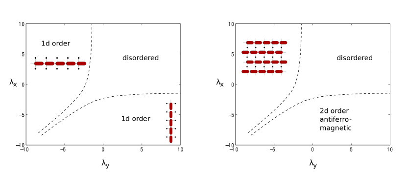
The physics becomes more interesting when the tilt $\vec{E}=(E_{x},E_{y})$ deviates slightly from the diagonal, $E_{x}\neq E_{y}$. Dipoles in $x$ direction and dipoles in $y$ direction now do not cost the same energy, and we define $\Delta_{x}=U-E_{x}$ ($\Delta_{y}=U-E_{y}$) the energy associated with a dipole in $x$ ($y$) direction.

In the limit $\Delta_{y}\rightarrow\infty$; $\Delta_{x}/\Delta_{y}\rightarrow 0$ the system can reduce its potential energy by maximizing the number of dipoles in $y$ direction; no dipoles in $x$ direction are created in the ground state. Thus the system decouples into a collection of horizontally aligned chains. In the absence of vertical dipoles these chains cannot interact with each other, and so each of them undergoes an independent 1d Ising transition as a function of $\Delta_{x}$ (see Fig. 2).

In this paper we study the full phase diagram of the near-diagonally tilted decorated square lattice. An important question is whether there is a region in the phase diagram where 2d order develops, i.e. whether a coupling develops between the above mentioned chains. We find that for realistic system sizes the crossover looks like the one of a collection of independent 1d chains. This is due to the fact that the inter-chain coupling is small compared to the finites-size gap of each chain between the symmetric and anti-symmetric superposition of its two ground states. There is thus no 2d order. A schematic phase diagram for this situation is shown in Figure 2a. The situation is different in the thermodynamic limit. As the finite-size gap vanishes the inter-chain coupling dominates, causing the chains to align anitferromagnetically. The schematic phase diagram in the thermodynamic limit is shown in Figure 2a.

The remainder of this paper is organized as follows. In Section II we introduce the model and describe the effective resonant subspace. In Section III we study the system by quantum Monte-Carlo (QMC) simulations and find no sign of a coupling between the chains. In Section IV we will show by exact diagonalization of a model system consisting of only two chains that there is indeed a very small coupling between these chains, which arises from processes in very high order in perturbation theory. We present conclusions in Section V.

II Model

In this section we describe the effective resonant subspace of a near-diagonally tilted decorated square lattice. We begin by recalling the Hamiltonian of a tilted Mott insulator. It is described by the generalized bosonic Hubbard model with an additional potential gradient along a certain direction, $H=H_{\rm kin}+H_{\rm U}+H_{\rm tilt}$:

$$H_{\rm kin} = -t\sum_{<ij>}\left(\hat{b}^{\dagger}_{i}\hat{b}_{j}+\hat{b}^{\dagger}_{j}\hat{b}_{i}\right)$$ (1a)

$$H_{\rm U} = \frac{U}{2}\sum_{i}\hat{n}_{i}(\hat{n}_{i}-1)+\frac{U_{3}}{6}\sum_{i}n_{i}(n_{i}-1)(n_{i}-2)+\dots$$ (1b)

$$H_{\rm tilt} = -E\sum_{i}{\bf e}\cdot{\bf r}_{i}\,\hat{n}_{i}.$$ (1c)

Here $\hat{b}_{i}$ are canonical boson operators on lattice sites $i$ at spatial co-ordinate ${\bf r}_{i}$, and $\hat{n}_{i}\equiv\hat{b}^{\dagger}_{i}\hat{b}_{i}$. The first term in $H_{\rm U}$ describes two-body interaction. The second term is an effective three-body interaction, generated by virtual processes involving higher bands multibody ; threebody ; three-body-Johnson . Such a term is present in ultracold atomic systems, and dramatically changes the physics of a tilted lattice, as we have shown in Ref. PielawaTiltMI, : if $U_{3}$ is not negligible compared to other energy scales in the problem, then this term causes processes which create triply occupied sites to be off-resonant. This effect is independent of the sign of $U_{3}$. Indeed, in recent cold atom experiments $U_{3}$ has been measured to be negativemultibody ; threebody ; GreinerPhotoAssistedTunneling . The potential gradient is $E$, and the fixed vector ${\bf e}$ is normalized so that the smallest change in potential energy between neighboring lattice sites has magnitude $E$. We assume that the potential drop per lattice site $E$ is comparable to the on-site repulsion $U$. The tilt has now two components $\vec{E}=(E_{x},E_{y})$, we define $\Delta_{x}=U-E_{x}$ and $\Delta_{y}=U-E_{y}$, and we work in the parameter regime where

$$\left|\Delta_{x}\right|,\left|\Delta_{y}\right|,t\ll\left|U\right|,\left|E\right|,\left|U_{3}\right|.$$ (2)

We assume that the parent Mott insulator has filling factor one atom per lattice site. The effective resonant subspace of the near-diagonally tilted decorated square lattice is then described by the Hamiltonian

$$\hat{H} = \Delta_{x}\sum_{i\in\textrm{x-links}}\hat{d}^{\dagger}_{i}\hat{d}_{i}+\Delta_{y}\sum_{j\in\textrm{y-links}}\hat{d}^{\dagger}_{j}\hat{d}_{j}-\sqrt{2}t\sum_{a}\left(\hat{d}_{a}+\hat{d}^{\dagger}_{a}\right),$$ (3)

here $\hat{d}^{\dagger}_{a}$ ($\hat{d}_{a}$) creates (annihilates) a dipole on a link $a$; where the first sum runs only over links aligned in $x$ direction, the second sum only over links aligned in $y$ direction. These two terms describe the energy cost/gain for having a dipole. The last sum comes from the hopping term and describes creation and annihilation of dipoles; it runs over all links. The dipoles obey a hard-core constraint: there can be no more than one dipole on each link. Additionally there is a constraint which does not allow dipoles to overlap on a site: each lattice site can be part of no more than one dipole.

For following discussion, we define the two independent tuning parameters

$$\lambda_{x} = \frac{\Delta_{x}}{\sqrt{2}t},\qquad\lambda_{y}=\frac{\Delta_{y}}{\sqrt{2}t}$$ (4)

These two parameters can take all real values.

II.1 Description by a constrained five-state model

Figure 3: Effective five-state model: each unit cell of the decorated square lattice can be in one out of five possible states: having no dipole, or having a dipole on one of the four links. There is also a constraint that dipoles may not overlap: two neighboring unit cells may not have dipoles directed towards each other. Thus the effective model is a constraint five state model on a simple square lattice.

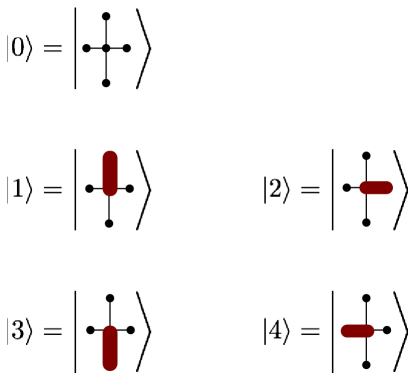
We can describe the resonantly connected subspace for all values of our tuning parameters $\lambda_{x}$ and $\lambda_{y}$ by a constrained five-state model on a simple square lattice. We let our unit cell be centered about the sites with four neighbors. Each of the unit cells may be in one out of five states, see Fig. 3: It may contain no dipole (state $\left|0\right\rangle$), or it may contain one dipole, and there are four links to choose from (states $\left|1\right\rangle$, $\left|2\right\rangle$, $\left|3\right\rangle$, $\left|4\right\rangle$). The Hamiltonian of a single site is then given by

$$H_{{\rm site}} = H_{{\rm pot}}+H_{{\rm kin}}$$

$$H_{{\rm pot}} = \lambda_{x}\left(\left|2\right\rangle\left\langle 2\right|+\left|4\right\rangle\left\langle 4\right|\right)+\lambda_{y}\left(\left|1\right\rangle\left\langle 1\right|+\left|3\right\rangle\left\langle 3\right|\right)$$

$$H_{{\rm kin}} = -\left|0\right\rangle\left(\left\langle 1\right|+\left\langle 2\right|+\left\langle 3\right|+\left\langle 4\right|\right)+{\rm h.c.}.$$ (5)

Summing over all sites we obtain the free Hamiltonian of the five state system

$$H_{{\textrm{free}}}=\sum_{x,y=1}^{L_{x},L_{y}}H_{{\rm site}}(x,y).$$

Additionally there is a constraint that the dipoles may not overlap: two neighboring unit cells may not point toward each other. We take this into account by projecting out all the states which would create such a collision

$$H^{c}=P_{c}H_{{\rm{free}}}P_{c}$$

where $P_{c}$ is a projection operator which projects out all the states that are forbidden by the constraint.

II.2 Mapping to a frustrated Ising spin model

In Refs.  SachdevMI, and GreinerIsing, , the physics of a tilted one-dimensional Mott Insulator was described by an antiferromagnetic Ising spin chain in a transverse and longitudinal field. In the same spirit, we map the diagonally tilted decorated square lattice to an antiferromagnetic spin model, also in longitudinal and transverse field, on a frustrated lattice. Note that the spin degrees of freedom reside on the links of the decorated square lattice, so that the lattice of the spin model is an ‘octagon-square-cross’ lattice as depicted in Fig. 1. This lattice has four sites per unit cell, and each spin has $z_{\rm{coord}}=4$ neighbors. As the lattice is not bipartite, an antiferromagnetic spin model on this lattice is frustrated, and two-dimensional Ising order is not possible. The Hamiltonian of the resonant subspace can be described by the following spin model

$$H = J\left(\sum_{\langle i,j\rangle}S_{z}^{i}S_{z}^{j}-h^{\rm{LR}}_{z}\sum_{i\in\rm LR}S_{z}^{i}-h^{\rm{UD}}_{z}\sum_{i\in\rm UD}S_{z}^{i}-h_{x}\sum_{i}S^{i}_{x}\right)$$ (6a)

$$h^{\rm{LR}}_{z} = \left(2-\frac{\Delta_{x}}{J}\right),\qquad h^{\rm{UD}}_{z}=\left(2-\frac{\Delta_{y}}{J}\right)$$ (6b)

$$h_{x} = 2\sqrt{2}\frac{t}{J}$$ (6c)

where $\vec{S}=\frac{1}{2}\vec{\sigma}$. The second sum ($i\in\rm{LR}$) is over all spins which reside on lines in horizontal direction, see Fig. 1, and the third sum ($i\in\rm{UD}$) is over spins that reside on vertical lines. While the first three terms all commute with each other, the last term does not. It is this transverse field which makes this a quantum problem. The strong antiferromagnetic interaction and the strong longitudinal field are introduced to realize the constraint: having two neighboring spin down costs an energy of order $J$. The mapping becomes exact in the limit $J\rightarrow\infty$. As in one dimension, this is of course not a mapping of the full bosonic model to a spin model, but of the resonantly connected subspace.

We will phrase most of the following discussion in the language of the constrained five-state model, keeping in mind that the results can directly be applied to the frustrated Ising spin model.

II.3 Limiting cases

We understand the system in the following limiting cases

1. $\lambda_{x},\lambda_{y}\rightarrow\infty$, $\lambda_{x}/\lambda_{y}=1$ (weak diagonal tilt): The parent Mott insulator is stable to a weak tilt, and so the dipole vacuum is the ground state in this limit. Dipole creation costs a large amount of energy, and so dipoles are only virtually created.

2. $\lambda_{x},\lambda_{y}\rightarrow-\infty$, $\lambda_{x}/\lambda_{y}=1$ (strong diagonal tilt): This is the quantum liquid state described in Ref. PielawaTiltMI, . The number of dipoles is maximized, and the ground state is an equal amplitude superposition of all dipole product states that fulfill the constraint. As we have shown in Ref. PielawaTiltMI, this is a disordered state; the ground state is unique and gapped.

3. $\lambda_{y}\rightarrow+\infty$; $\lambda_{x}/\lambda_{y}\rightarrow 0$: along this line vertical dipole states on links aligned in $y$ direction cannot be occupied, as they cost an infinite amount of energy, while horizontal dipoles along links in $x$ direction are accessible. In this limit the system decouples into a collection of horizontal one-dimensional chains. These chains are effectively one-dimensional, they undergo a phase transition in the Ising universality class at a critical value of $\lambda_{x}=-1.31$ (which is the same as in the one-dimensional case).

We expect the one-dimensional order within each chain to persist when $\lambda_{y}$ takes on finite values. Neighboring chains may then interact via dipole states aligned in $y$ direction, which might lead to a coupling between these chains, and thus to two-dimensional order.

III Phase diagram obtained from Quantum Monte Carlo

Here we present results from a Quantum Monte Carlo study of the effective resonant subspace of the near-diagonally tilted decorated square lattice. We emphasize that we do not simulate the full bosonic Hamiltonian: QMC would then look for the absolute ground state, which means that all bosons follow the tilt and fall down to minus infinity. Instead we simulate the effective resonant subspace, which is described by the constrain five state model.

III.1 Order parameters

As we expect one-dimensional order to persist in some region of the phase diagram, we introduce order parameters which probe for 1D Ising order, as well as order parameters which probe for two-dimensional order.

Before introducing our order parameters, we begin by reviewing the order parameter of the one-dimensional system in Refs. SachdevMI, ; GreinerIsing, : a staggered magnetization which breaks lattice symmetries (translation, inversion, and reflection symmetry). In the language of the spin mapping in Section II.2, and Ref. GreinerIsing, it is given by

$$M=\frac{1}{L}\sum_{l}(-1)^{l}\sigma_{l}^{z}.$$

In the limit $\lambda_{y}=\infty$, $\lambda_{x}/\lambda_{y}=0$ each unit cell of the decorated square lattice has only three states available, and we can directly translate this staggered magnetization to our notation. Each chain aligned along the $x$ direction and at position $y$ then has its own, independent order parameter

$$M_{{\rm LR}}(y)=\frac{1}{L_{x}}\sum_{x}\left(\hat{p}_{\rightarrow}-\hat{p}_{\leftarrow}\right)_{x,y}=\frac{1}{L_{x}}\sum_{x}m_{{\rm LR}}(x,y),$$ (7)

where $\hat{p}_{d}$ is a projection operator that projects onto the dipole state $d.$ Note that this order parameter is normalized to take values in the interval $[-1,1]$. The (staggered) magnetization of each unit cell has been defined for dipoles along left-right direction only as

$$m_{{\rm LR}}(x,y)=\hat{p}_{\rightarrow}-\hat{p}_{\leftarrow}$$

When $\lambda_{y}\neq\infty,$ each unit cell has two additional states available. We can still use the above definition, and add another component to the order parameter,

$$m_{{\rm UD}}(x,y)=\hat{p}_{\downarrow}-\hat{p}_{\uparrow}$$

the magnetization for dipoles aligned in y direction. We combine the two to a vector,

$$\vec{m}(x,y)=\left(\begin{array}[]{c}m_{{\rm LR}}(x,y)\\ m_{{\rm UD}}(x,y)\end{array}\right)$$

we will refer to this as the “magnetization” of a unit cell of our system. The magnetization $\vec{m}(x,y)$ transforms as a vector and is odd under inversion. To probe for two-dimensional order in the system, we define the total magnetization

$$\vec{M}=\frac{1}{L_{x}L_{y}}\sum_{x,y}\vec{m}(x,y).$$ (8)

and measure $\langle\vec{M}^{2}\rangle$. If the chains are aligned ferromagnetically, then this order parameer is non-zero. To probe for antiferromagnetically aligned chains we define a total staggered magnetization

$$\vec{M}_{{\rm stagg,x}} = \frac{1}{L_{x}L_{y}}\sum_{x,y}(-1)^{x}\vec{m}(x,y),$$

$$\vec{M}_{{\rm stagg,y}} = \frac{1}{L_{x}L_{y}}\sum_{x,y}(-1)^{y}\vec{m}(x,y).$$

For an anisotropic tilt we expect the most important effect to be an order within each chain. These chains may or may not be coupled to form two-dimensional order. It is therefore usefull to define order parameters which probe for one-dimensional order along $x$ or $y$ direction only. For this purpose we will use $M_{{\rm LR}}(y)$, Eq. 7, and average its square over all chains,

$$\langle\langle M_{{\rm LR}}^{2}\rangle\rangle = \frac{1}{L_{y}}\sum_{y}\langle M_{{\rm LR}}^{2}(y)\rangle=\frac{1}{L_{x}}\frac{1}{L_{y}^{2}}\sum_{x,x^{\prime},y}\langle m_{{\rm LR}}(x,y)m_{{\rm LR}}(x^{\prime},y)\rangle$$ (9)

and similarly for for chains aligned along $y$, $\langle\langle M_{{\rm UD}}^{2}\rangle\rangle=\frac{1}{L_{x}}\sum_{x}\langle M_{{\rm UD}}^{2}(x)\rangle.$

III.2 Phase diagram

Figure 4: Phase diagram obtained from QMC study. We find only one-dimensional order. The two-dimensional order parameters are zero everywhere. The phase boundary was obtained from crossing of the BinderbinderCumulant cumulant of the one-dimensional magnetization, Eq. (9), see Appendix A.1. Square lattice of size $L_{x}=L_{y}=(4,8,16,32,64)$ the imaginary time slice thickness was $a=0.04$, imaginary time direction was scaled with the linear system size, $M_{\tau}=(40,80,160,320,640)$, corresponding to temparatures $T=(0.625,0.3125,0.1562,0.0781,0.0391).$ Essentially the same phase diagram is obtained from order parameter scaling assuming the Ising exponent $\eta=1/4.$

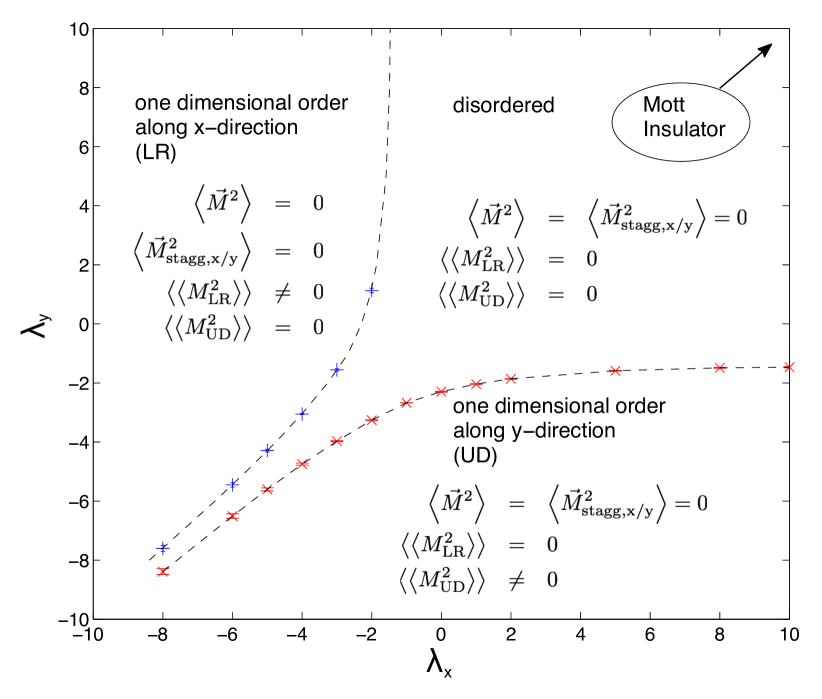
Results of the QMC simulations are summarized in the phase diagram shown in Figure 4. The disordered dipole state for $\lambda_{x},\lambda_{y}\rightarrow-\infty$ appears to be continuously connected to the parent Mott insulator at $\lambda_{x},\lambda_{y}\rightarrow+\infty$ . There is a critical line where the system undergoes a transition to an ordered state with one dimensional order along individual chains. For $\lambda_{y}<\lambda_{x}$ these chains are aligned in $y$ direction (lower right corner of the phase diagram in Fig. 4), and $\langle\langle M_{{\rm UD}}^{2}\rangle\rangle\neq 0,$ while $\langle\vec{M}{}^{2}\rangle=\langle\vec{M}_{{\rm stagg,x}}^{2}\rangle=\langle\vec{M}_{{\rm stagg,y}}^{2}\rangle=0.$ We will show below that the system indeed seems to be disordered in the transverse direction; each chain appears to have a two-fold degenerate ground state, which is independenent of the order parameters of the neighboring chains, and so the two-dimensional system has a ground state degeneracy $2^{L_{x}}$, where $L_{x}$ is the linear system size in $x$ direction, i.e. the number of chains. Correlations in the $x$ direction decay exponentially with a correlation length which is smaller than the lattice spacing, $\xi_{x}\ll a$. There is no region in the phase diagram where either $\langle\vec{M}{}^{2}\rangle$, Eq. 8, or $\langle\vec{M^{2}}_{{\rm stagg,x}}\rangle$ or $\langle\vec{M^{2}}_{{\rm stagg,}y}\rangle$ takes a non-zero value.

We probe for two-dimensional order by measuring $\langle\vec{M}^{2}\rangle$. This quantity scales with system size exactly as it would for a collection randomly aligned magnetized one-dimensional chains. This suggests that there is no two-dimensional order: while in some regions of the phase diagram there is long range order along individual chains, there is no correlation between these chains, see Figure 5.

Figure 5: Absence of two dimensional order in the QMC study. Here we show the scaling of the total magnetization with system size, $\langle\vec{M}^{2}\rangle\times L$. For randomly aligned magnetized chains we expect $\langle\vec{M}^{2}\rangle\propto 1/L$, while for perfectly aligned chains $\langle\vec{M}^{2}\rangle={\rm const}$ and for antiferromagnetic order in transverse direction $\langle\vec{M}^{2}\rangle=0$. In the disordered phase $\langle\vec{M}^{2}\rangle\propto 1/(L_{x}L_{y})$. This shows that in the ordered phase the system behaves as a collection of independent chains with one-dimensional order within each chain. Here $\lambda_{x}=-5$ was kept fixed; similar results are obtained for different cuts through the phase diagram.

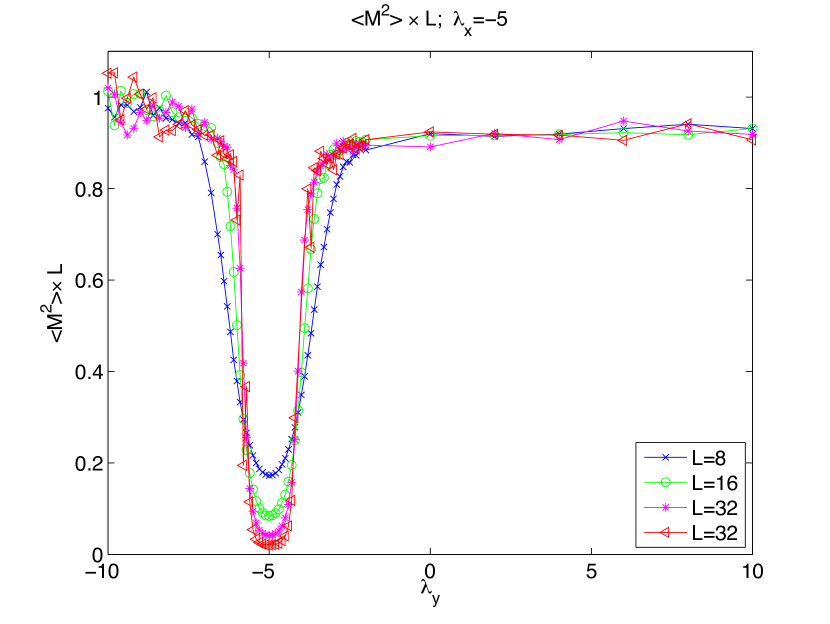
We find good data collapse with the critical exponents of the 2D classical Ising model (Onsager exponents), see Appendix. This further supports the observation that individual chains behave as independent 1d Ising systems.

Note that this QMC method can also be used for a “doped” system, i.e. a system with initial defects in the Mott insulator. Defected sites then block neighboring links from dipole occupation. Studying such a disordered system is an interesting subject to future work.

IV Inter chain coupling: Exact diagonalization study

Quantum Monte Carlo results describe a system which decouples into a collection of one-dimensional chains, while on symmetry grounds one would expect that a coupling between the chains should be generatedSubirBook . The following scenarios might explain this disagreement

• hidden symmetry: there could be a subtle microscopic symmetry which forbids any coupling between the order parameters of the chains. The next relevant term is then the energy-energy coupling, which leads to a change of the critical exponent $\nu$ but no ordering of the chains; or

• finite-size effects: the coupling between the chains could be present, but is too small to have an observable effect for the system sizes studied with QMC. Simulating larger lattices should then, in principle, find a phase with two-dimensional order.

Here we resolve this question by an exact diagonalization study of a toy model, which consists of two chains and qualitatively captures the interchain constraint, and thus the coupling.

We find that a coupling between two neighboring chains is indeed present: it is antiferromagnetic in sign and very small in magnitude. It appears only in high order in perturbation theory in $t/|U-E|$, and is thus not observable for realistic system sizes, neither in QMC nor in cold-atomic quantum simulation experiments.

IV.1 Toy model

We use a simplified model with only two chains. We reduce the Hilbert space further by only keeping the three most relevant dipole states in each unit cell, see Figure 6. The state without dipole has been integrated out, while one of the vertical dipole states is missing: this enhances the coupling and reduces the size of the Hilbert space, which enables us to study longer chains. We expect this toy model to qualitatively describe the interchain coupling of our system.

Figure 6: Two chain model used for the exact diagonalization study. Each central site (marked with a square) can be in one out of three states. A chain of length four unit cells is shown. This model should capture the interchain behavior of our model qualitatively.

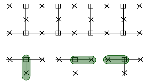
The Hamiltonian for each of a single unit cell reads

$$H_{{\rm site}}=\left(\begin{array}[]{ccc}\Delta_{b}&-t_{b}&-t_{b}\\ -t_{b}&\Delta_{a}&-t_{a}\\ -t_{b}&-t_{a}&\Delta_{a}\end{array}\right)$$

where $\Delta_{a}$ is the energy cost for a dipole along chain direction, and $\Delta_{b}$ is the energy cost for a dipole in direction transverse to the chains. The effective hopping elements $t_{a},$ and $t_{b}$ are obtained from second order perturbation theory, and they both have a negative sign (since $\Delta_{a}<\Delta_{b}<0$):

$$t_{b} = t^{2}\left(\frac{1}{\Delta_{a}}+\frac{1}{\Delta_{b}}\right),$$ (10)

$$t_{a} = \frac{2t^{2}}{\Delta_{a}}.$$ (11)

In addition to the single site Hamiltonian, there is the hard-core constraint forbidding two central sites from pointing toward each other. This constraint reduces the size of the Hilbert space.

IV.2 Results

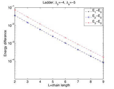
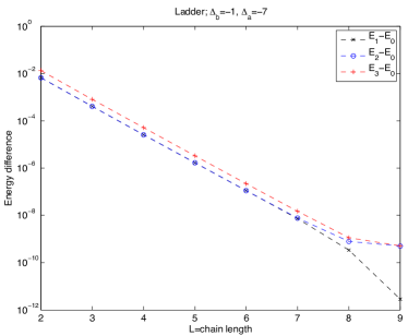
We diagonalized this system for a chains of up to length nine, with periodic boundary conditions. The chain length $L$ refers to the number of unit cells in each chain. In analyzing the results, it is useful to compare the spectrum to that of a simple model of two decoupled Ising chains in the ordered phase. For systems of finite length, this model would give four low-energy states, whose splitting vanishes exponentially with the system size in the thermodynamic limit.

Fig. 7 shows the energy of the three lowest excited states relative to the ground state, as a function of the system size. At first glance, these results are consistent with the model of completely decoupled chains, since the energy splitting to the three lowest excited states appears to vanish exponentially. However, for certain parameters and for the longest systems (Fig. 7b), we observe a deviation from the decoupled chain model. Two of the low-energy states remain nearly degenerate, while the gap to the other two starts deviating from exponential. This behavior is consistent with having a small but non-zero inter-chain coupling.

Figure 7: Strong finite-size effects: Logarithmic plot for energy of the first three excited states relative to the ground state as a function of system length, for (a) $\Delta_{a}=-5,\Delta_{b}=-4$ (b) $\Delta_{a}=-7,\Delta_{b}=-1$. The lines $E_{1}-E_{0}$ and $E_{2}-E_{0}$ appear on top of each other. At first sight this suggests that there are four ground states in the thermodynamic limit and that thus the order parameters of the chains are not coupled. However there is a small splitting between the first two levels above the ground state. As can be seen in Fig. 8 this splitting grows linearly with system size and eventually dominates over the finite-size gap for long enough chains.

IV.2.1 Estimate of the order parameter coupling

The following observations further support the existence of a small coupling between the order parameters of the two chains:

1. There is a splitting between the first and the second excited state, $E_{2}-E_{1}$. This splitting is too small to be visible in Fig. 7a. We present it in Fig. 8. Although the magnitude of the splitting is very small, it grows approximately linearly with system size, consistent with a finite energy density associated with an inter-chain order parameter coupling.
   

   

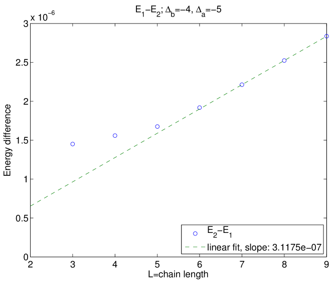
   Figure 8: Splitting between first and second excited state grows linearly with system size. This suggests that there is indeed a coupling between the order parameters of these two chain.

2. We can show that there is no hidden symmetry forbidding order parameter coupling: if we fix the boundary conditions to make the chains either aligned or anti-aligned, there is a difference in ground state energy of these two systems which grows linearly with system size, see Fig.  9. We can use the slope of this curve as an estimate for the coupling of the order parameters per unit cell.
   

   

   

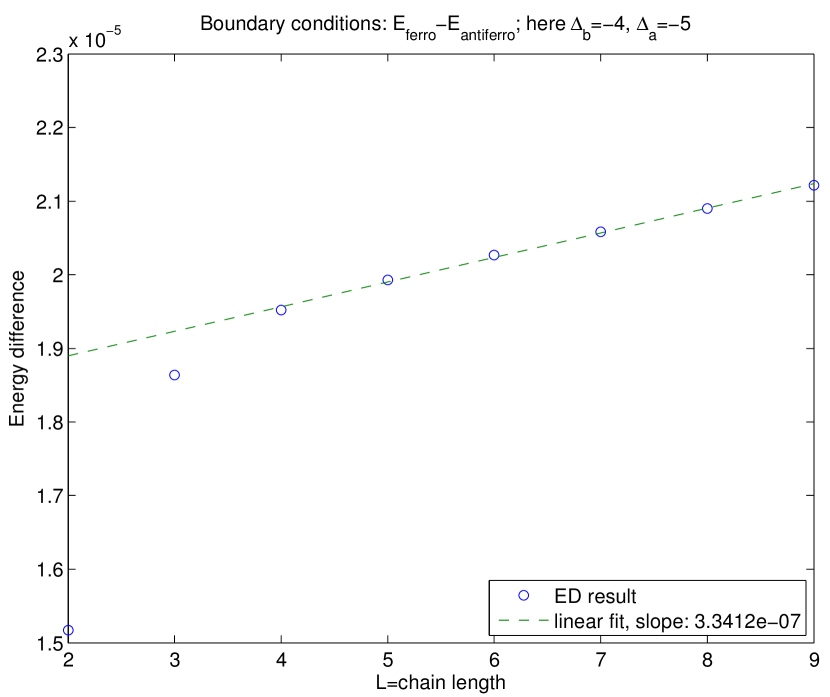
   Figure 9: The inter-chain coupling is antiferromagnetic, which we show by fixing the boundary conditions so that the chains are forced to be either aligned or anti-aligned. The energy difference grows linearly with system size and antiferromagnetic boundary conditions are energetically favorable.

The slopes of both curves in Fig. 7,9 agree approximately, giving us a good estimate for the order parameter coupling of the chains. For the system sizes we studied, however, this coupling is smaller than the effective tunneling element between the different ground states, i.e. smaller than the finite-size gap. For larger chains this order parameter coupling will start to dominate over the tunneling, and then there will only be two ground states. The coupling between two chains is antiferromagnetic.

IV.2.2 Estimate of order in perturbation theory for coupling

We now estimate the order in perturbation theory in which the antiferromagnetic coupling is generated. To this end, we set $t_{a}=t_{b}=1$ and use $\Delta=\Delta_{b}-\Delta_{a}$ as our only tuning parameter. Let $E_{c}$ be the energy per unit length of the antiferromagnetic coupling

$$E_{c}=\frac{E_{2}-E_{1}}{N}$$

(here $N$ is the chain length). If the antiferromagnetic coupling appears roughly in $n$th order in perturbation theory, then

$$E_{c} \propto \left|\Delta\right|^{1-n}$$ (12)

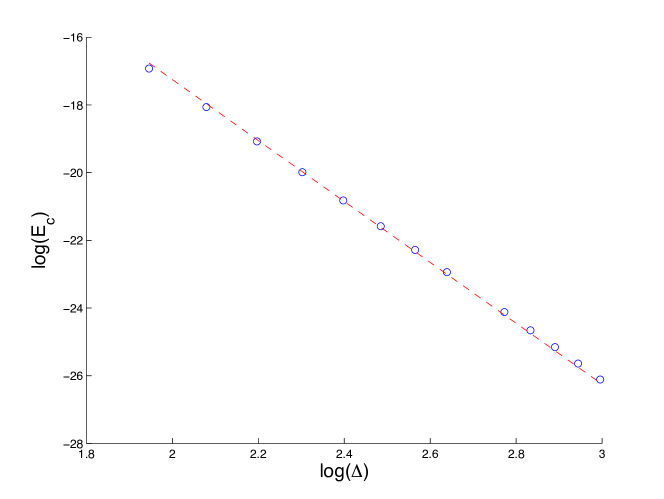
$$\log\left(E_{c}\right) = (1-n)\log\left(\left|\Delta\right|\right)+\rm{const}$$ (13)

We plot $\log{E_{c}}$ versus $\log(\left|\Delta\right|)$ and obtain $n=10$ from a linear fit (see Fig. 10). This suggests that the antiferromagnetic inter-chain coupling is generated roughly in 10th order in perturbation theory within this toy model, and in 20th order in perturbation theory within the bosonic model.

Figure 10: The antiferromagnetic coupling appears in 10th order in perturbation theory. This logarithmic plot shows that the coupling per unit length scales as $\left|\Delta\right|^{-9}$, where $\Delta=\Delta_{b}-\Delta_{a}$.

IV.3 Mechanism for inter-chain coupling

Having established that, in the ordered phase, the chains couple antiferromagnetically, it is natural to ask what is the microscopic mechanism responsible for this coupling. Below, we give a qualitative argument for the generation of inter-chain coupling in high orders in $t/\Delta$, which predicts that the sign of the coupling should be antiferromagnetic.

We begin by the observation that in the Ising ordered phase, there are two distinct types of domain wall fluctuations, a kink and an anti-kink (see Fig. 11(a,b)). Kink-anti-kink pairs can be generated virtually, lowering the kinetic energy. We note also that the two domain walls have a parametrically different effective mass: the kink (Fig. 11a) can hop via a process of order $t_{b}^{2}/(|\Delta_{a}-\Delta_{b}|)$, while the anti-kink (Fig. 11b) is much lighter, hopping via a process of order $t_{a}$. Therefore, the anti-kinks are more delocalized. We note also that kink-anti-kink pairs in a fully ordered configuration are created with a preferred orientation. For example, if the order parameter in a particular chain is pointing to the left, then each kink is typically to the right of its anti-kink partner (see Fig 11c). As a consequence, world lines of kinks curve in the opposite direction than world lines of anti-kinks; and which way they curve is determined by the sign of the order parameter. Some typical space-time paths of fluctuating kink-anti-kink pairs are shown schematically in Fig. 11c.

The order parameters of two neighboring chains are not coupled directly; i.e., in a classical, fully ordered configuration (which is the ground state in the limit $t_{a,b}=0$), there is no energy difference between an aligned and an anti-aligned configuration. However, in the presence of quantum fluctuations, the two chains become coupled. For instance, in our two-chain model, kinks cannot occur simultaneously on both chains, because of the constraint preventing two dipoles to point towards each other. Note that there is no such constraint for anti-kinks; configurations in which anti-kinks in the two chains occur on the same rung are allowed.

Figure 11: A kink (a) and anti-kink (b) configuration. Kinks in different chains cannot reside on the same rung, because of the hard-core constraint; no such restriction exists for the anti-kinks. c) Schematic space-time trajectories for kink-anti-kink pairs. The kinks (anti-kinks) are represented by solid (dashed) lines, respectively. The arrows represent the direction of the Ising order parameter. The average order parameter is assumed to be pointing to the left. In this configuration, the kinks are typically to the right of the anti-kinks, and their world lines typically curve left. Since the two chains couple only through the kinks, this provides a mechanism for coupling the order parameters of the two chains. d,e) A simplified model showing the source of the interaction between the order parameters of the two chains. The space-time trajectories of kinks on the upper chain are approximated, for simplicity, by the rectangular U-shaped curves shown in blue. We define the “position” of a world line as the center of the rectangle enclosing it. The hatched region shows the space-time volume blocked for the position of kinks in the lower chain, assuming that the order parameters of the two chains are aligned (d) or anti-aligned (e), due to the hard core repulsion between kinks in the upper and lower chains. The space-time trajectories of kinks in the lower chain in the two cases are shown by the dashed blue curves.

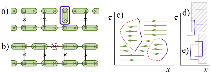
This hard-core interaction between kinks provides a mechanism for coupling the order parameters of the two chains. Consider the kink space-time configuration in Fig. 11c. In this configuration the world lines of kinks tend to curve to the right, because of the hard-core repulsion between kinks and anti-kinks on the same chain. The repulsive interaction between kinks on two neighboring chains reduces the “phase space” available for quantum fluctuations. However, one can imagine that if the two order parameters are anti-aligned, the phase space for fluctuations is slightly larger than in the opposite case. This is since if the order parameters are anti-aligned, the space-time trajectories of the kinks on the lower chain tend to curve oppositely to those of on the upper chain, allowing one to fit more quantum fluctuations in a given space-time “volume” (thus lowering the kinetic energy). To see this, imagine for simplicity that the space-time trajectories of kinks in the upper chain are of the shape shown by the solid blue curve in Fig. 11d. Then, one can ask how much space-time volume does a kink in the upper chain block for kinks in the lower chain. The blocked volume is twice as large in the case in which the order parameters of the two chains are aligned, compared to the anti-aligned case (Fig. 11d,e), favoring the order parameters to be anti-aligned. This “order by disorder” mechanism explains how the repulsion between kinks can generate a coupling between the order parameters of the two chains to high order in $t_{a,b}/|\Delta_{a}-\Delta_{b}|$. Moreover, it predicts that the coupling is antiferromagnetic, consistently with the ED findings described above. We believe that it is unlikely that this coupling could introduce new phases.

V Conclusions

We have proposed a setup to simulate frustrated quantum Ising spins with cold atoms in a tilted optical lattice, by generalizing an idea which has been successfully applied experimentally in one dimension. We have studied the phase diagram of the resulting model and found that it has strong finite-size effects. For realistic systems it decouples into a collection of one dimensional Ising chains, a coupling between the chains is present in the thermodynamic limit. A quantum simulator of ultracold atoms would, however, be limited in the system size. We therefore expect it to observe a one-dimensional transition to ordered chains, just as we did in QMC.

Appendix A Details on the QMC study

We mapped the two-dimensional quantum model Eq. (3) to three-dimensional classical model with discrete imaginary time. The model has now become a three-dimensional constraint five-state model on a cubic lattice. In the Monte Carlo simulations we used single site flips (which change the state of a unit cell), as well as cluster updates (i.e. updates which flip a segment in imaginary time at a given spatial position, and updates that flip the magnetization of an entire chain). Time discritization introduces a Trotter error, but it should change neither the nature of the phases, nor the universality class of the phase transition.

For the results presented in this paper we used an imaginary time slice thickness $a=0.04$; we have also run simulations with smaller imaginary time slices and obtained similar results. We had 27000 equilibration sweeps before starting to take measurements. Mearsurements were taken every 50 sweeps, and 50 measurements were binned into one group. The number of groups were (2290, 1090, 530, 210) for linear system size (8, 16, 32, 64). Error bars were obtained from a simple binning analysisBinderMCbook .

A.1 Binder cumulant

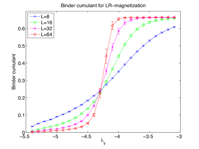
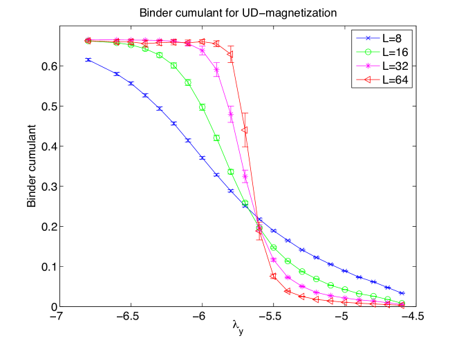
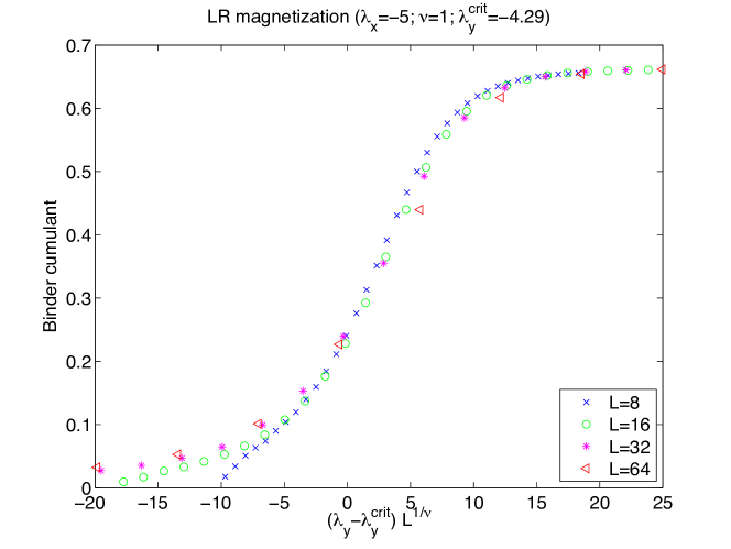
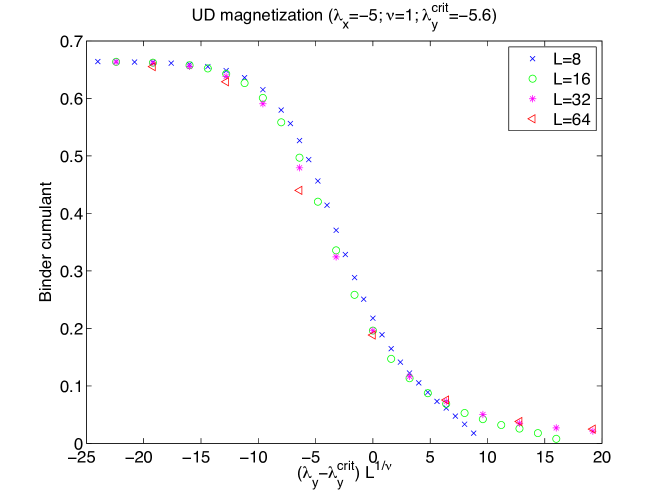
The Binder cumulant gives a good estimate for the critical point, and it does not depend on critical exponents binderCumulant . For an Ising order parameter, $M$, the Binder cumulant is defined as

$$U=1-\frac{\left\langle M^{4}\right\rangle}{3\left\langle M^{2}\right\rangle^{2}}.$$

When the Binder cumulant is plotted for different system sizes, all curves should cross at the critical point for the following reason. While for an infinite system the magnetization vanishes at the critical point as

$$M\propto\left(-\tau\right)^{\beta},$$

where $\tau$ is the reduced temperature $\tau=T/T_{c}-1$, $\beta$ is the critical exponent of the magnetization. For a finite system there are corrections to scaling, described by a scaling function $\phi$, which only depends on $\xi/L$,

$$M=\left(-\tau\right)^{\beta}\phi\left(\xi/L\right)=\left(-\tau\right)^{\beta}\tilde{\phi}\left(\tau L^{1/\nu}\right),$$

where $\xi$ is the correlation length, and $\nu$ is the correlation length exponent. We used $\xi=\tau^{-\nu}$ to rewrite the scaling function for a different argument. The average magnetization squared, and raised to the fourth power, have different scaling functions,

$$\left\langle M^{2}\right\rangle = \left(-\tau\right){}^{2\beta}u_{2}\left(\tau L^{1/\nu}\right)$$

$$\left\langle M^{4}\right\rangle = \left(-\tau\right){}^{4\beta}u_{4}\left(\tau L^{1/\nu}\right)$$

and so the Binder cumulant is a function of this same argument, $\tau L^{1/\nu}$

$$U(\tau,L)=1-\frac{u_{4}\left(\tau L^{1/\nu}\right)}{3\left(u_{2}\left(\tau L^{1/\nu}\right)\right)^{2}}=f\left(\tau L^{1/\nu}\right),$$ (14)

At the critical point we have $\tau=0$, and so the Binder cumulant at this point should not depend on system size. In the thermodynamic limit for an Ising system in the ordered phase $U\rightarrow\frac{2}{3}$, and $U\rightarrow 0$ in the disordered phase. Fig. 12 shows the Binder cumulant of the one-dimensional order parameters $\langle\langle M_{LR}^{2}\rangle\rangle$ and $\langle\langle M_{UD}^{2}\rangle\rangle$ for different cuts through the phase diagram.

Figure 12: Binder cumulant for order parameters $\langle\langle M_{{\rm LR}}^{2}\rangle\rangle$ and $\langle\langle M_{{\rm UD}}^{2}\rangle\rangle$ for a horizontal cut through the phase diagram, keeping $\lambda_{x}=-5$ fixed, plotted for different system sizes, $L_{x}=L_{y}=8,\>16,\>32,\>64.$ Similar plots are obtained for different cuts through the phase diagram.

A.2 Order parameter scaling and the critical exponent $\eta$

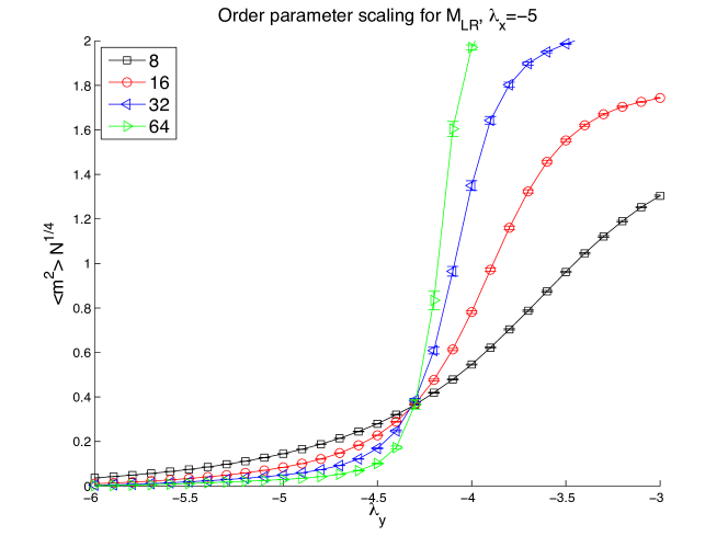
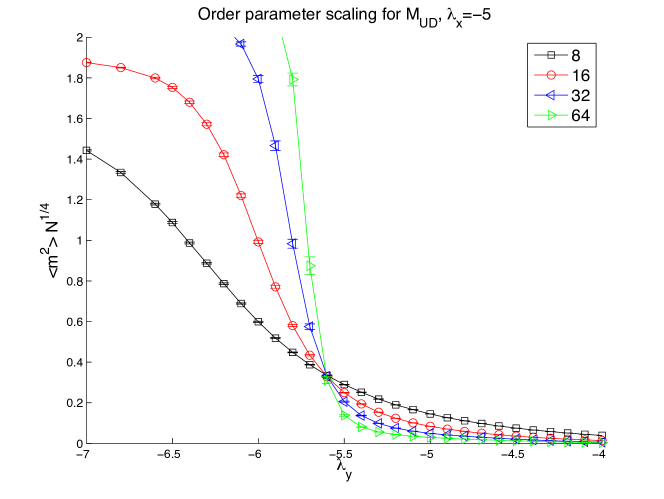
The phase transition point can also be found from order paramter scaling. This will depend on the correlation length exponent, $\eta$. Let $M$ again be an Ising order parameter, at the critical point the correlation decays as a power law,

$$\langle M(r)M(0)\rangle \propto \left|\vec{r}\right|^{-(d+z-2+\eta)}$$ (15)

$z$ is the dynamic critical exponent, which is $z=1$ in case of the Ising model. We define M as the (normalized) total magnetization $M=1/L\int M(r)dr$, and for a one dimensional system ($d=1$) we have

$$\langle M^{2}\rangle\propto L^{-\eta}$$ (16)

The correlation length exponent for the 2D classical Ising model is $\eta=1/4.$ In Figure 13 we plot $\langle\langle M_{LR}^{2}\rangle\rangle L^{-1/4}$ and $\langle\langle M_{UD}^{2}\rangle\rangle L^{-1/4}$ for different system sizes. The crossing point of these lines gives us the phase boundary which agrees with the one found from the Binder cumulant.

Figure 13: Order parameter scaling, assuming the correlation length exponent $\eta=1/4$ of the classical two-dimensional Ising model. Good agreement of the crossing points, also with the ones found from the Binder cumulant.

A.3 Critical exponent $\nu$

If we rescale the $x$ axis for the Binder cumulant, and plot it as a function of $\left(\lambda-\lambda_{c}\right)L^{1/\nu}$, then the data points for all system sizes should collapse. We indeed observe a good data collapse for the correlation length exponent of the classical two-dimensional Ising model, $\nu=1$, see Fig. 14.

Figure 14: Data collapse for the critical exponent $\nu=1$ of the classical two-dimensional Ising model. The $x$ axis is centered around the critical point and rescaled by $L^{1/\nu}$

References

- (1) D. Jaksch, C. Bruder, J. I. Cirac, C. W. Gardiner, and P. Zoller. Cold Bosonic Atoms in Optical Lattices. Phys. Rev. Lett. 81, 3108–3111 (Oct 1998).
- (2) Immanuel Bloch, Jean Dalibard, and Wilhelm Zwerger. Many-body physics with ultracold gases. Rev. Mod. Phys. 80, 885–964 (Jul 2008).
- (3) Immanuel Bloch, Jean Dalibard, and Sylvain Nascimbène. Quantum simulations with ultracold quantum gases. Nature Physics 8 (April), 267–276 (2012).
- (4) J Ignacio Cirac and Peter Zoller. Goals and opportunities in quantum simulation. Nature Physics 8 (April), 264–266 (2012).
- (5) Markus Greiner, Olaf Mandel, Tilman Esslinger, Theodor W. Hansch, and Immanuel Bloch. Quantum phase transition from a superfluid to a Mott insulator in a gas of ultracold atoms. Nature 415 (6867), 39–44 (2002).
- (6) Ehud Altman, Walter Hofstetter, Eugene Demler, and Mikhail D Lukin. Phase diagram of two-component bosons on an optical lattice. New Journal of Physics 5 (1), 113 (2003).
- (7) A. B. Kuklov and B. V. Svistunov. Counterflow Superfluidity of Two-Species Ultracold Atoms in a Commensurate Optical Lattice. Phys. Rev. Lett. 90, 100401 (Mar 2003).
- (8) M. Guglielmino, V. Penna, and B. Capogrosso-Sansone. Ising antiferromagnet with ultracold bosonic mixtures confined in a harmonic trap. Phys. Rev. A 84, 031603 (Sep 2011).
- (9) Assa Auerbach. Interacting Electrons and Quantum Magnetism. Springer (1994).
- (10) S. Trotzky, P. Cheinet, S. F lling, M. Feld, U. Schnorrberger, A. M. Rey, A. Polkovnikov, E. A. Demler, M. D. Lukin, and I. Bloch. Time-Resolved Observation and Control of Superexchange Interactions with Ultracold Atoms in Optical Lattices. Science 319 (5861), 295–299 (2008).
- (11) Subir Sachdev, K. Sengupta, and S. M. Girvin. Mott insulators in strong electric fields. Phys. Rev. B 66, 075128 (2002).
- (12) Paul Fendley, K. Sengupta, and Subir Sachdev. Competing density-wave orders in a one-dimensional hard-boson model. Phys. Rev. B 69, 075106 (Feb 2004).
- (13) Jonathan Simon, Waseem S Bakr, Ruichao Ma, M Eric Tai, Philipp M Preiss, and Markus Greiner. Quantum simulation of antiferromagnetic spin chains in an optical lattice. Nature 472 (7343), 307–312 (April 2011).
- (14) Waseem S. Bakr, Jonathon I. Gillen, Amy Peng, Simon Folling, and Markus Greiner. A quantum gas microscope for detecting single atoms in a Hubbard-regime optical lattice. Nature 462 (7269), 74–77 (2009).
- (15) Jacob F. Sherson, Christof Weitenberg, Manuel Endres, Marc Cheneau, Immanuel Bloch, and Stefan Kuhr. Single-atom-resolved fluorescence imaging of an atomic Mott insulator. Nature 467 (7311), 68–72 (2010).
- (16) Nathan Gemelke, Xibo Zhang, Chen-Lung Hung, and Cheng Chin. In situ observation of incompressible Mott-insulating domains in ultracold atomic gases. Nature 460 (7258), 995–998 (August 2009).
- (17) Tatjana Gericke, Peter Wurtz, Daniel Reitz, Tim Langen, and Herwig Ott. High-resolution scanning electron microscopy of an ultracold quantum gas. Nat Phys 4 (12), 949–953 (December 2008).
- (18) Karl D. Nelson, Xiao Li, and David S. Weiss. Imaging single atoms in a three-dimensional array. Nat Phys 3 (8), 556–560 (August 2007).
- (19) K. Sengupta, Stephen Powell, and Subir Sachdev. Quench dynamics across quantum critical points. Phys. Rev. A 69, 053616 (May 2004).
- (20) M. Kolodrubetz, D. Pekker, B. K. Clark, and K. Sengupta. Nonequilibrium dynamics of bosonic Mott insulators in an electric field. Phys. Rev. B 85, 100505 (Mar 2012).
- (21) Chester P. Rubbo, Salvatore R. Manmana, Brandon M. Peden, Murray J. Holland, and Ana Maria Rey. Resonantly enhanced tunneling and transport of ultracold atoms on tilted optical lattices. Phys. Rev. A 84, 033638 (Sep 2011).
- (22) Susanne Pielawa, Takuya Kitagawa, Erez Berg, and Subir Sachdev. Correlated phases of bosons in tilted frustrated lattices. Phys. Rev. B 83, 205135 (2011).
- (23) Sebastian Will, Thorsten Best, Ulrich Schneider, Lucia Hackermuller, Dirk-Soren Luhmann, and Immanuel Bloch. Time-resolved observation of coherent multi-body interactions in quantum phase revivals. Nature 465, 197–201 (2010).
- (24) P R Johnson, E Tiesinga, J V Porto, and C J Williams. Effective three-body interactions of neutral bosons in optical lattices. New Journal of Physics 11, 093022 (2009).
- (25) P R Johnson, D Blume, X Y Yin, W F Flynn, and E Tiesinga. Effective renormalized multi-body interactions of harmonically confined ultracold neutral bosons. New Journal of Physics 14 (5), 053037 (2012).
- (26) Ruichao Ma, M. Eric Tai, Philipp M. Preiss, Waseem S. Bakr, Jonathan Simon, and Markus Greiner. Photon-Assisted Tunneling in a Biased Strongly Correlated Bose Gas. Phys. Rev. Lett. 107, 095301 (2011).
- (27) K. Binder. Finite size scaling analysis of Ising model block distribution functions. Zeitschrift für Physik B Condensed Matter 43, 119–140 (1981).
- (28) Subir Sachdev. Quantum Phase Transitions. Cambridge University Press (2011).
- (29) Kurt Binder and Dieter W. Heermann. Monte Carlo Simulation in Statistical Physics. Springer (2010).