The clustering of galaxies in the SDSS-III Baryon Oscillation Spectroscopic Survey: Baryon Acoustic Oscillations in the Data Release 9 Spectroscopic Galaxy Sample
Abstract
We present measurements of galaxy clustering from the Baryon Oscillation Spectroscopic Survey (BOSS), which is part of the Sloan Digital Sky Survey III (SDSS-III). These use the Data Release 9 (DR9) CMASS sample, which contains massive galaxies covering square degrees with an effective redshift and redshift range . Assuming a concordance CDM cosmological model, this sample covers an effective volume of 2.2 Gpc3, and represents the largest sample of the Universe ever surveyed at this density, . We measure the angle-averaged galaxy correlation function and power spectrum, including density-field reconstruction of the baryon acoustic oscillation (BAO) feature. The acoustic features are detected at a significance of in both the correlation function and power spectrum. Combining with the SDSS-II Luminous Red Galaxy Sample, the detection significance increases to . Fitting for the position of the acoustic features measures the distance to relative to the sound horizon at . Assuming a fiducial sound horizon of , which matches cosmic microwave background constraints, this corresponds to a distance . At 1.7 per cent, this is the most precise distance constraint ever obtained from a galaxy survey. We place this result alongside previous BAO measurements in a cosmological distance ladder and find excellent agreement with the current supernova measurements. We use these distance measurements to constrain various cosmological models, finding continuing support for a flat Universe with a cosmological constant.
keywords:
cosmology: observations, distance scale, large-scale structure1 Introduction
Explaining the late-time acceleration of the expansion rate of the Universe (Riess et ali., 1998; Perlmutter et al., 1999) is one of the most perplexing problems in modern physics. All known attempts require exotic ingredients: a new, very small energy scale in a cosmological constant or low-mass field, a change to General Relativity to weaken gravity on large scales or at low densities, or extra dimensions of space-time. Empirical observations will provide clues as to the cause by providing precision measurements of the expansion history and the growth of cosmological structure over time (e.g. Kolb et al., 2006).
One of the key methods for measuring the expansion history is to use features in the clustering of galaxies within galaxy surveys as a ruler with which to measure the distance–redshift relation. Obtaining precision distance measurements is a long-standing challenge in astronomy, and the Baryon Acoustic Oscillations (BAO) signal in the two-point clustering of galaxies provides a particularly robust quantity to measure. The BAO arise because the coupling of baryons and photons by Thomson scattering in the early universe allows acoustic oscillations at early times, which in turn leads to a rich structure in the distribution of matter and the anisotropies of the cosmic microwave background (CMB) radiation. The distance that acoustic waves can propagate in the first million years of the universe becomes a characteristic comoving scale (Peebles & Yu 1970; Sunyaev & Zel’dovich 1970; Doroshkevich et al. 1978; a description of the physics leading to the features can be found in Eisenstein & Hu 1998 or Appendix A of Meiksin, White & Peacock 1999 and a discussion of the acoustic signal in configuration space can be found in Eisenstein et al. 2007b). As the acoustic signature is imprinted on very large scales ( Mpc) it is quite insensitive to astrophysical processing that occurs on smaller scales, thus BAO experiments are affected by a very low level of systematics induced by such processes. Recent reviews of BAO as a probe of dark energy may be found in Eisenstein (2008) and Weinberg et al. (2012).
This acoustic signature has now been detected in many different galaxy surveys, using a variety of methods to analyse the evolved density field (Percival et al., 2001; Miller, Nichol & Batuski, 2001; Eisenstein et al., 2005; Cole et al., 2005; Hutsi, 2006; Padmanabhan et al., 2007; Blake et al., 2007; Percival et al., 2007c; Okumura et al., 2008; Gaztanaga, Cabre & Hui, 2009; Kazin et al., 2010; Percival et al., 2010; Reid et al., 2010; Blake et al., 2011a; Beutler et al., 2011; Seo et al., 2012; Padmanabhan et al., 2012a), and it is already producing stringent constraints on cosmological models. Constraints can be obtained from either photometric or spectroscopic samples, though for the same volume and number of galaxies the spectroscopic samples provide much stronger constraints. The first BAO measurements came from the 2dF Galaxy Redshift Survey (2dFGRS; Colless et al. 2003) and the Sloan Digital Sky Survey (SDSS; York et al. 2000); when combined, the most recent analyses give a 2.7 per cent measurement of the distance-redshift relation at (e.g. Percival et al., 2010). Adding to these data, Blake et al. (2011a) measured the BAO feature at , using the WiggleZ survey (Drinkwater et al, 2010), making a 4 per cent distance measurement from galaxies. This result was subsequently improved to provide distance measurements of accuracy 7.2 per cent, 4.5 per cent and 5.0 per cent in three bins centered at redshifts , , and respectively, using the full sample of galaxies from this survey (Blake et al., 2011b). Beutler et al. (2011) made a 4.5 per cent measurement at with the 6dF Galaxy Redshift Survey (6dFGRS: Jones et al. 2009). Thus the BAO technique has recently provided a distance–redshift relation at a series of redshifts both higher and lower than the 2dFGRS and SDSS measurements.
The BAO signal in an evolved galaxy field, such as those analysed in the papers described above, differs from that predicted in the matter field by linear theory alone. The dominant difference is caused by matter flows and peculiar velocities on intermediate scales (), which act to suppress small-scale oscillations in the galaxy power spectrum and smooth the BAO feature in the correlation function (Eisenstein et al., 2007b; Crocce & Scoccimarro, 2008; Matsubara, 2008a, b). Eisenstein et al. (2007a) suggested that this smoothing can be reversed, in effect using the phase information within the density field to reconstruct linear behaviour. Although not a new idea (e.g. Peebles, 1989, 1990; Nusser & Dekel, 1992; Gramann, 1993), the dramatic effect on BAO recovery had not been previously realised, and the majority of the benefit was shown to be recovered from a simple reconstruction prescription. This reconstruction technique has been used to sharpen the BAO feature and improve distance constraints on mock data (Padmanabhan & White, 2009; Noh, White & Padmanabhan, 2009; Seo et al., 2010; Mehta et al., 2011), and it was recently applied to the SDSS-II Luminous Red Galaxy (LRG) sample (Padmanabhan et al., 2012a). The reconstruction was particularly effective in this case, providing a 1.9 per cent distance measurement at , decreasing the error by a factor of 1.7 compared with the pre-reconstruction measurement.
This study is the first in a set of papers to describe the clustering of galaxies at from Data Release 9 (DR9) of the Baryon Oscillation Spectroscopic Survey (BOSS; Schlegel, White & Eisenstein, 2009), which is part of SDSS-III (Eisenstein et al., 2011). We present cosmological results based on fits to the BAO signature in the clustering of galaxies in this paper. Redshift-Space Distortion (RSD) and Alcock-Paczynski (Alcock & Paczynski, 1979, AP) measurements are presented in Reid et al. (2012), and an interpretation of these results in terms of dark energy and modified gravity models is presented in Samushia et al. (2012). Tojeiro et al. (2012a) describe a new method for improving RSD measurements. Further constraints from fitting models to the full shape of the correlation function are presented in Sanchez et al. (2012). Nuza et al. (2012) have compared the clustering with the outcome of a large-volume cosmological simulation.
Each of these papers focusses on the high redshift galaxy sample from BOSS, denoted “CMASS”, where a set of colour-magnitude cuts are used to select a roughly volume-limited sample of massive, luminous galaxies from a redshift of to . We describe the construction of the galaxy catalog and measurement of both the correlation function and power spectrum of this sample, before and after applying the reconstruction algorithm of Eisenstein et al. (2007a). We present the results of two pipelines for the analysis of BAO: one utilising the correlation function, and one utilising the power spectrum. While both statistics contain the same information, they often have different advantages in the usage and application in the literature. We compare and contrast measurements made on mock catalogues using both techniques, and apply both to measure and analyse the BAO distance scale using CMASS data. In companion papers we present weights used to correct for artificial density fluctuations caused by observational effects (Ross et al., 2012) and a set of mock catalogues used to estimate statistical errors (Manera et al., 2012). An analysis of a lower redshift sample of galaxies from BOSS will be presented in Parejko et al. (2012). Clustering measurements from a smaller sample of CMASS galaxies (the first six months of BOSS data) were presented by White et al. (2011) and used to constrain halo occupation distributions, but these measurements did not extend to the BAO scale.
The layout of our paper is as follows. We introduce the data in Section 2 and the catalogue used in Section 3. Analysis techniques are described in Section 4, and correlation function and power spectrum measurements are described and presented in Sections 5 and 6, respectively. These are compared and our final distance measurement presented in Section 7. This measurement is placed in a cosmological context in Sections 8 and 9. A brief discussion is given in Section 10. Finally, a series of Appendices test the validity of various aspects of the methods used.
Throughout the paper we assume a fiducial CDM+GR111We do not consider any modifications to general relativity in this paper. flat cosmological model with , , , and , similar to the best-fit WMAP 7-year model (Komatsu et al., 2011). These parameters allow us to translate angles and redshifts into distances and provide a reference against which we measure distances. The BAO measurement allows us to constrain changes in the distance scale relative to that predicted by this fiducial model.
2 The Data
The Sloan Digital Sky Survey (SDSS; York et al., 2000) mapped over one quarter of the sky using the dedicated 2.5-m Sloan Telescope (Gunn et al., 2006) located at Apache Point Observatory in New Mexico. A drift-scanning mosaic CCD camera (Gunn et al., 1998) imaged the sky in five photometric bandpasses (Fukugita et al., 1996; Smith et al., 2002; Doi et al., 2010) to a limiting magnitude of . The imaging data were processed through a series of pipelines that perform astrometric calibration (Pier et al., 2003), photometric reduction (Lupton et al., 2001), and photometric calibration (Padmanabhan et al., 2008). The magnitudes were corrected for Galactic extinction using the maps of Schlegel, Finkbeiner & Davis (1998). BOSS, as part of the SDSS-III survey (Eisenstein et al., 2011), has imaged an additional square degrees of sky over that of SDSS-II (Abazajian et al., 2009) in the South Galactic sky, in a manner identical to the original SDSS imaging. This increased the total imaging SDSS footprint to square degrees, with square degrees at deg in the North Galactic Cap and square degrees at deg in the South Galactic Cap. All of the imaging was re-processed as part of SDSS Data Release 8 (Aihara et al., 2011).
BOSS is primarily a spectroscopic survey, which is designed to obtain spectra and redshifts for 1.35 million galaxies over an extragalactic footprint covering square degrees. These galaxies are selected from the SDSS imaging and are being observed together with quasars and approximately ancillary targets. The targets are assigned to tiles of diameter using a tiling algorithm that is adaptive to the density of targets on the sky (Blanton et al., 2003). Aluminium plates are drilled with holes whose positions correspond to the positions of objects on each tile, which are manually plugged with optical fibres that feed a pair of double spectrographs. The double-armed BOSS spectrographs are significantly upgraded from those used by SDSS-I/II, covering the wavelength range Å to Å with a resolving power of to (Gunn et al., 2012). In addition to expanding the wavelength coverage from the SDSS-I range of to Å, the throughputs have been increased with new CCDs, gratings, and improved optical elements, and the -fibre cartridges with apertures have been replaced with -fibre cartridges with apertures. Each observation is performed in a series of -second exposures, integrating until a minimum signal-to-noise ratio is achieved for the faint galaxy targets. This ensures a homogeneous data set with a high redshift completeness of per cent over the full survey footprint. A summary of the survey design appears in Eisenstein et al. (2011), and a full description will be provided in Dawson et al. (2012).
2.1 Galaxy target selection
BOSS makes use of luminous galaxies selected from the multi-colour SDSS imaging to probe large-scale structure at intermediate redshift (). The target selection is an extension of the targeting algorithms for the SDSS-II (Eisenstein et al., 2001) and 2SLAQ (Cannon et al., 2006) Luminous Red Galaxies (LRGs), targeting fainter and bluer galaxies in order to achieve the a number density of . The majority of the galaxies have old stellar systems whose prominent 4000 Å break makes them relatively easy to target using multi-colour data. The details of the target selection algorithm will be presented in Padmanabhan et al. (2012b); we summarise the details relevant to this paper below.
The galaxy target selection in BOSS is divided into two classes of galaxies: LOWZ galaxies () and CMASS galaxies (), analogous to the Cut-I and II SDSS-II LRGs. The 4000 Å break resides primarily in the and bands for the LOWZ and CMASS redshift ranges respectively. The LOWZ sample in DR9 was somewhat compromised by a target selection error, now fixed, in the early data, and regardless it would have fewer objects and a lower effective volume than the SDSS-II LRGs over the same redshift range. We therefore restrict our analysis here to the CMASS sample and use the results from Padmanabhan et al. (2012a) for measurements in the lower redshift range. The small scale clustering results of the LOWZ sample is described in the companion paper of Parejko et al. (2012). Future BOSS analyses will use both the LOWZ and CMASS samples.
The CMASS sample was designed to loosely follow a constant stellar mass cut (hence the name ConstantMASS) based on the passive galaxy template of Maraston et al. (2009), and was designed to produce a uniform mass distribution at all redshifts. The distribution of CMASS stellar masses (Maraston et al., 2012) and velocity dispersions (Thomas et al., 2012) in various redshift bins confirm that this goal was achieved. Unlike SDSS-II LRGs, we do not exclusively target intrinsically red galaxies with the CMASS cut. In fact, Masters et al. (2011) showed that 26 per cent of CMASS galaxies are massive spirals. Therefore, whereas both the LOWZ and CMASS samples are colour-selected, CMASS is a significantly more complete sample than LOWZ at high stellar masses. This issue is discussed in detail in Tojeiro et al. (2012a), which considers the passive evolution of galaxies between the SDSS-II Luminous Red Galaxies (which form a subset of the LOWZ sample) and the CMASS sample. Most CMASS objects are central galaxies residing in dark matter halos of , but a non-negligible fraction are satellites that live primarily in halos about 10 times more massive (White et al., 2011; Nuza et al., 2012). Galaxies in the CMASS sample are highly biased (), and bright enough to be used to trace a large cosmological volume with sufficient number density to ensure that shot-noise is not a dominant contributor to the statistical error in BAO measurements. The combination of large volume, high bias, and reasonable space density makes CMASS galaxies particularly powerful for probing statistical properties of large-scale structure.
The CMASS target selection makes use of four definitions of flux computed by the photometric pipeline. All magnitudes have been photometrically calibrated using the uber-calibration of Padmanabhan et al. (2008) and corrected for Galactic extinction (Schlegel, Finkbeiner & Davis, 1998). The model fluxes are computed using either a PSF-convolved exponential or de Vaucouleurs light profile fit to the -band only, and are denoted with the subscript. Cmodel fluxes are computed using the best-fit linear combination of an exponential and a de Vaucouleurs light profile fit to each photometric band independently (Abazajian et al., 2009), and are denoted with the subscript . Point-spread function (PSF) fluxes are computed by fitting a PSF model to the galaxy, and are denoted with the subscript (Stoughton et al., 2002). Fibre fluxes are computed within a 2 arcsec aperture after the image is convolved with a kernel to produce a 2 arcsec FWHM PSF, and are denoted with the subscript . Colours are computed using model fluxes. Magnitude cuts are performed on cmodel and fibre fluxes.
The CMASS algorithm selects luminous galaxies at , extending Cut II of Eisenstein et al. (2001) to both fainter and bluer galaxies. We first select objects classified as galaxies by the imaging pipeline. These must then pass the following criteria:
| (1) | |||||
| (2) | |||||
| (3) | |||||
| (4) | |||||
| (5) |
where the auxiliary colour is defined as (Cannon et al., 2006)
| (6) |
CMASS objects must also pass the following star-galaxy separation cuts
| (7) | |||||
| (8) |
unless they also pass the LOWZ criteria (see Ross et al. 2012; Parejko et al. 2012), which only uses the default SDSS-II star-galaxy separation criterion. Stars will have essentially identical model and PSF fluxes, and this star-galaxy separation cuts on the difference between these two magnitudes. The slope with apparent magnitude in equations 7 and 8, which is not used in the standard star-galaxy separator of the photometric pipeline (Strauss et al., 2002), was set empirically by analysing commissioning spectroscopic data that relaxed these cuts. Our choices yield a sample with approximately 3 per cent stellar contamination, and it discards approximately 1 per cent of genuine galaxy targets, mostly at the faint end. The star-galaxy separation is known to fail when the seeing is poor, as PSF and model magnitudes approach one another for all object types in poor seeing. However this has been shown to have negligible effect on the angular distribution of targets in SDSS (Ross et al., 2011).
2.2 Masks
We use the Mangle software (Swanson et al., 2008) to track the areas covered by the BOSS survey and the angular completeness of those regions. The mask is constructed of spherical polygons, which form the base unit for the geometrical decomposition of the sky. The angular mask of the survey is formed from the intersection of the imaging boundaries (expressed as a set of polygons) and spectroscopic sectors (areas of the sky covered by a unique set of spectroscopic tiles) (see Blanton et al., 2003; Tegmark et al., 2004; Aihara et al., 2011).
In addition to tracking the outline of the survey region and the position of the spectroscopic plates, we apply several “vetos” in constructing the catalog. Regions were masked where the imaging was unphotometric, the PSF modelling failed, the imaging reduction pipeline timed out (usually due to too many blended objects in a single field), or the image was identified as having critical problems. Small regions around the centre posts of the plates where fibres cannot be placed due to physical limitations and around bright stars in the Tycho catalog (Høg et al., 2000) were also masked. The mask radius for stars from the Tycho catalog was
| (9) |
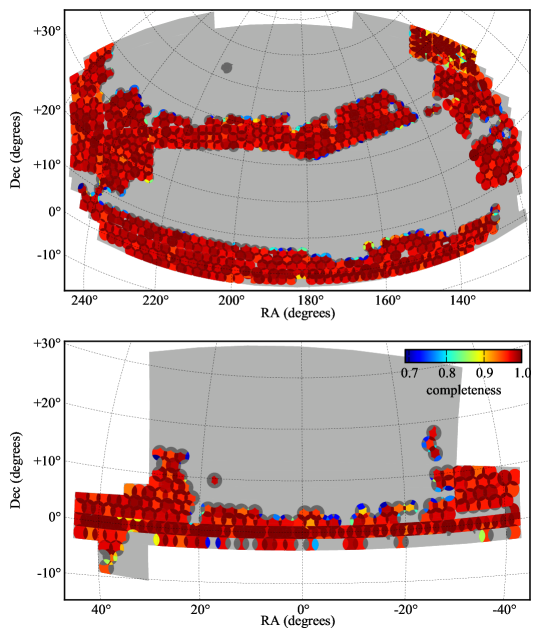
where is the Tycho magnitude clipped to fall in the range . We also place a mask at the locations of objects with higher priority (mostly high- quasars) than galaxies. A galaxy cannot be observed at a location within the fibre collision radius of these points. In total we masked per cent of the area cover by the set of observed tiles due to our “veto” mask. The sky coverage of the CMASS galaxies is shown in Fig. 1, and the basic parameters including areas and galaxy numbers are presented in Table 1.
2.3 Measuring galaxy redshifts
Spectroscopic calibration, extraction, classification, and redshift analysis were carried out using the v5_4_45 tag of the idlspec2d software package.222http://www.sdss3.org/svn/repo/idlspec2d/tags/v5_4_45/. The classification and redshift of each object are determined by fitting their coadded spectra to a set of galaxy, quasar, and star eigentemplates. The fit includes a polynomial background (quadratic for galaxies, quasars, and cataclysmic variable stars; cubic for all other stars) to allow for residual extinction effects or broadband continua not otherwise described by the templates. The reduced versus redshift is mapped in redshift steps corresponding to the logarithmic pixel scale of the spectra, . Galaxy templates are fit from to , quasar templates are fit from to , and star templates are fit from to (kms-1). The template fit with the best reduced is selected as the classification and redshift, with warning flags set for poor wavelength coverage, broken/dropped and sky-target fibres, and best fits which are within of the next best fit (comparing only to fits with a velocity difference of less than 1000 kms-1). This method is the same as used for the SDSS DR8; see Aihara et al. (2011) for further explanation.
For galaxy targets, a dominant source of false identifications is due to quasar templates with unphysical fit parameters, e.g., large negative parameters causing a quasar template emission feature to fit a galaxy absorption feature. Thus, for galaxy targets, the best classification and redshift are selected only from the fits to galaxy and star templates, and we restrict to fits the pipeline classifies as robust. 333 These fits are stored in the “*_NOQSO” versions of the Z, Z_ERR, ZWARNING, CLASS, SUBCLASS, and RCHI2DIFF fields in the upcoming Data Release 9. This analysis uses Z_NOQSO redshifts for targets selected with CLASS_NOQSO=“GALAXY” and ZWARNING_NOQSO=0.
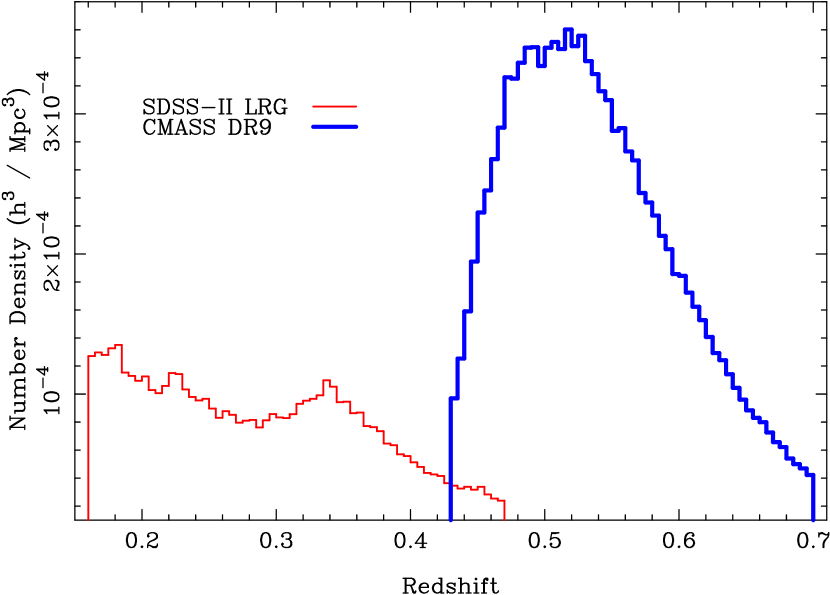
Fig. 2 shows the galaxy number density of the CMASS sample, compared with the SDSS-II LRG sample. The CMASS galaxies have approximately three times the density of the SDSS-II LRG sample, and sample the underlying density field with lower noise and higher fidelity. Although redshifts are recovered at higher and lower redshifts, we limit the CMASS redshift range to : at lower redshifts the BOSS LOWZ sample is more dense, and we wish to remove overlap between samples. At , the efficiency with which we recover redshifts decreases, potentially leading to increased systematic errors (Ross et al., 2012).
3 Catalog creation
3.1 Target photometry
Target galaxies are selected as described in Section 2.1 based on the best reduced photometry available at the time of target selection. All imaging data used by BOSS is based on photometry from SDSS Data Release 8 (DR8; Aihara et al. 2011). During the early phases of BOSS, the final DR8 imaging data were still being processed, and therefore some of the SDSS imaging (9 per cent) used for targeting CMASS galaxies is now designated as secondary444i.e. there is an overlapping observation with higher quality photometry in the DR8 database. Although the measured object parameters from different observing runs over the same region agree within the photometric errors, there can be significant differences between target samples selected from these different observing runs. These differences between our target catalog and that obtained using DR8 primary photometry arise due to the stochastic variations one expects given the magnitude errors and the different photometry. We have therefore produced a “combined photometry target” sample that uses the photometry input to each run of the targeting software. Thus, rather than thinking of the set of BOSS CMASS galaxies as being a unique sample of galaxies chosen with the properties described in Section 2.1, we should really consider the stochastic nature caused by photometric errors: we are simply observing one of the samples that could have been selected with these properties: using different imaging data we would find a different sample. We do not expect this issue to have any impact on the analysis or results presented here, as it is stochastic in nature. We only include this description for completeness and to aid future uses of these data.
3.2 Close-pair corrections
The protective sheath around each spectroscopic fibre and the ferrule that holds the fiber in the plug plate has a diameter of 62′′ on the focal plane, so no two objects separated by less than this can be observed on a single plate. This means that groups and clusters of galaxies with members closer than this apparent separation will be systematically under-sampled, strongly affecting the measured small-scale clustering signal if uncorrected. The targeting algorithm has been designed to place a fibre on as many objects within tight groups as possible (The selection is random with respect to galaxy properties other than position on the sky). Where there are two plates covering a sector we find that approximately per cent of the pairs separated by only have one galaxy observed; this fraction reduces to per cent when a sector is covered by three or more plates. An algorithm that corrects for these effects on small scales is presented and tested in Guo et al. (2011). On large scales, this procedure is equivalent to upweighting the galaxies nearest to each unobserved galaxy, and we adopt this procedure in the analysis presented here. An alternative would have been to upweight all galaxies within the sector to compensate, which would have better shot-noise properties. However, the lost galaxies will predominantly be in groups, and thus may have different clustering properties than the average galaxy. We therefore accept the subsequent slightly increased shot-noise contribution. This close-pair correction weight is denoted throughout this paper (see also Section 3.7). For each target we set , and add one to this for each CMASS target within that failed to get a fiber allocated. This correction affects per cent of all the galaxies, with most of these in pairs with .
3.3 SDSS-II redshifts
Accurate redshifts for a subsample of the target galaxies were previously obtained within the SDSS-II survey (Abazajian et al., 2009). These galaxies were not re-observed by BOSS. We have redshift measurements for 100 per cent of the SDSS-II galaxy subsample by definition, and although these lie within the BOSS survey region, the angular distribution will systematically differ from that of the remaining subsample. We do not try to define a survey mask that amalgamates the SDSS-II and BOSS observations because the SDSS-II redshifts do not even form a random subsample of the BOSS targets based on galaxy properties. Instead, we subsample the SDSS-II galaxies to match the sector completeness of the galaxies observed within the BOSS program, where sector completeness is defined within each mask sector as
| (10) |
where , , and are defined in Section 3.5.
We also subsample the galaxies so that including the galaxies with previously known redshifts does not change the fraction of close pairs observed in any sector.This task is accomplished by calculating, for each sector, the fraction of close pairs within the sample of targets from which the known galaxies have been removed. We then subsample close pairs introduced when including the known galaxies, randomly removing either galaxy in a pair until the fraction of the introduced close pairs matches that of the sample without known galaxies.
Thus we force the known redshifts to have the same statistical properties as the BOSS galaxies within each sector, such that the angular distribution of the combined sample follows that of the BOSS angular mask.
3.4 Redshift-failure corrections
We do not achieve stellar classification or a good redshift determination for every spectrum taken. The probability of successfully obtaining an accurate spectrum is dependent on the fibre used - some fibres have degraded transmission, the optical quality (resolution) is better for spectra in some regions of the CCD than others, and the quality of the sky-subtraction is worse where the resolution is lower. Bundles of fibres are generally allocated to similar regions on the plates, and thus the failure rate is a strong function of position in the field-of-view for each observation. This effect is shown in Fig. 3 of our companion paper (Ross et al., 2012), where specific regions within each field-of-view are demonstrated to have worse-than-average failure probabilities. Our overall redshift success rate is 98.2 per cent, so we lack redshifts for a sufficiently small subsample that the effect on the measured clustering signal is very small.
We correct for this minor issue by upweighting the nearest (based on an angular search) target object for which a galaxy redshift, or stellar classification, has been successfully achieved. The redshift distribution of these nearest neighbours matches that of the full sample (see Fig. 4 of Ross et al. 2012), suggesting that the anisotropic component of the redshift-failure distribution which should be the difference between the two does not depend on redshift. Consequently, upweighting the nearest galaxy with a good redshift should match the true large-scale density and correct for the spatially dependent redshift failure effects. Further details can be found in Section 2.3 of Ross et al. (2012). This redshift-failure correction weight is denoted throughout this paper (see also Section 3.7). As in the case of , we define it to be unity for all galaxies and then add one if there is a nearby redshift failure.
3.5 Summary of target objects
| Property | NGC | SGC | total |
|---|---|---|---|
| 222 538 | 60 792 | 283 330 | |
| 3766 | 1810 | 5576 | |
| 7201 | 1771 | 8972 | |
| 3751 | 1122 | 4873 | |
| 14 116 | 3640 | 17 756 | |
| 4931 | 1911 | 6842 | |
| 207 246 | 57 037 | 264 283 | |
| 233 490 | 63 685 | 297 175 | |
| 256 303 | 71 046 | 327 349 | |
| Total area / deg2 | 2635 | 709 | 3344 |
| Effective area / deg2 | 2584 | 690 | 3275 |
To summarise, the following outcomes are available for BOSS targets that are covered by the survey:
-
1.
galaxies with redshifts from good BOSS spectra (we denote the number in each sector by ),
-
2.
galaxies with redshifts from SDSS-II spectra (),
-
3.
spectroscopically confirmed stars (),
-
4.
objects with BOSS spectra from which stellar classification or redshift determination failed (),
-
5.
objects with no spectra, in a close-pair (),
-
6.
objects with no spectra, or spectra removed following the subsampling discussed in Section 3.3, not in a close-pair ().
In the following we define the number of target objects per sector
| (11) |
and the number of targets observed per sector
| (12) |
The number of good galaxies used in the analysis per sector , is less than as we only use galaxies with . Table 1 gives the total split of galaxies in the CMASS DR9 target sample into these categories, where we define , and the areas and weighted areas for the CMASS sample in the Northern Galactic Cap (NGC) and Southern Galactic Cap (SGC), and combined as derived from the DR9 data.
Considering the numbers of galaxies in each category per sector, we can define a sector completeness as in Eq. 10, and the galaxies with previously known redshifts are subsampled to match this completeness, as well as the BOSS-only close-pair fraction as detailed in Section 3.3. The distribution of sector completenesses across the BOSS footprint is shown in Fig. 1. To remove sectors that have only been partially observed, we only retain sectors with greater than 70 per cent.
We also make a cut on the total redshift failure within each sector. First, we define a redshift completeness by
| (13) |
Then a sector is removed if it has more than 10 BOSS spectra, but fewer than 80 per cent of the non-stellar spectra have good redshift measurements (i.e. we remove sectors with and ). For these sectors we assume that there was a serious problem with the observations. Plate 3698 observed MJD 55501 is responsible for many redshift failures; it was poor data inadvertently included in DR9 with a CMASS failure rate of 23 per cent.
3.6 Systematic weights
Ross et al. (2011) have presented a critical examination of the large-scale angular clustering of CMASS target galaxies. They demonstrated that the density of stars has a significant effect on the observed density of galaxies, and this can introduce spurious fluctuations in the galaxy density field. This effect arises because stars have a large-scale power signature in their distribution across the sky. Additional potential systematics such as Galactic extinction, seeing, airmass, and sky background have also been investigated, and all have been found to potentially introduce spurious fluctuations into the galaxy density field, albeit to varying degrees. These non-cosmological fluctuations can be corrected for using a weighting scheme that minimises these fluctuations as a function of a given systematic effect (see Fig. 4 of Ross et al. 2011).
Ross et al. (2012) investigated systematic effects on the 3D clustering of the DR9 CMASS sample. They found that stellar density is the primary source of systematic error, and that computing a set of weights based on stellar density and magnitude alone has a similar effect as fitting for all five systematic sources simultaneously. Over-fitting these fluctuations can result in removing cosmological power, if the weights remove what are in truth statistical fluctuations. Hence the simplicity of correcting for one systematic only, with the added dependence on , minimises this risk. This approach was tested by making use of mock catalogues. We refer the reader to Ross et al. (2012) for a detailed study of the effect of all weighting schemes, and an analysis of each Galactic hemisphere separately. Note that Ross et al. (2012) explicitly verify that the BAO scale is insensitive to these systematic effects.
The adopted methodology for computing the angular systematic weights used throughout this paper is as follows. The weights are defined as
| (14) |
where is the stellar density. and are given by
| (15) | |||||
| (16) |
where the coefficients , , and were fitted so as to give a flat relation between galaxy density and . For , and were fixed at the values. These weights were applied to each galaxy individually, according to the stellar density of the patch of sky in which it lies, and to its observed . The stellar density map was computed using a HEALPix (Górski et al., 2005) grid with Nside = 256, which splits the sky into equal area pixels of 0.0525 deg This pixel size is much smaller than the scale at which the systematic effect of stars becomes important (), but large enough that the mean number of stars in a pixel is greater than 80 (implying any shot-noise effects will be small). As this is a large scale effect, a relatively coarse mask is sufficient.
3.7 Final weights and effective volume
As described in the previous sections, galaxies are weighted to allow for close-pair corrections with , redshift failures with and angular systematic weights with . We also apply weights to optimise our clustering measurements in the face of shot-noise and cosmic variance (Feldman, Kaiser & Peacock, 1994),
| (17) |
where is the mean density at redshift and . This ignores the scale dependence of the power spectrum and chooses a value optimised for the BAO feature, . We make this simplification for convenience; using the full scale-dependent weights proposed by Feldman, Kaiser & Peacock (1994) does not change our results and errors. Ross et al. (2012) find this weighting reduces the variance on the CMASS DR9 mock galaxy sample , typically by 20 per cent relative to no weighting. Combining with the systematic weights , the redshift-failure weights , and the close-pair weights , the final weights applied to the galaxies are given by
| (18) |
Here and are mutliplicative weights depending on spatial location, while and are additive weights, with default of unity. Using these weights, we calculate the effective volume using our fiducial cosmology as
| (19) |
where is the volume of the shell at (accounting for the observational area). We find for our CMASS sample which covers the redshift range . The weighted mean redshift of galaxies within the sample is , which we define as the effective redshift of our clustering measurements.
3.8 Random catalog generation
The evaluation of the correlation function and of the power spectrum requires an estimate of the average galaxy density. To provide such an estimate, we generate random catalogs of unclustered objects with the detailed redshift and angular selection functions of the sample, accounting for the complex survey geometry. In particular, the random catalogs account for the differences between the Northern and Southern Galactic Caps. To minimise the shot-noise induced on clustering measurements, these catalogues have times more objects than the corresponding galaxy catalogues. Numerous tests have confirmed that the survey selection function can be factorised into angular and redshift pieces (Ross et al., 2012). The redshift selection function can be taken into account by distributing the objects of the random catalogue according to the observed redshift distribution of the sample. We use the “shuffled” catalogue as defined in Ross et al. (2012), where the redshifts are matched to randomly selected galaxies. We do this separately for the NGC and SGC samples (see Appendix A for a further discussion of this). The completeness on the sky is determined from the fraction of target galaxies in a sector for which we obtained a spectrum, with the sectors being areas of the sky covered by a unique set of spectroscopic tiles (see Section 2.2). We upweight close pairs and redshift failures in the galaxy catalog as described in Section 3.4, and therefore include these targets when calculating the completeness for the random catalog. Thus the random catalogue was subsampled to the sector completeness as given by Eq. 10.
4 Analysis
We analyse the BAO feature and fit for a distance to using both the correlation function (Section 5) and power spectrum (Section 6) of the 3D galaxy distribution. The steps in both analyses parallel one another: (i) density-field reconstruction of the BAO feature, (ii) computation of the two-point statistics, (iii) estimation of errors on these measurements by analysing mock catalogs and (iv) extraction of a distance measurement by fitting the data. This section details these steps. Details specific to each method as well as the results are discussed in later sections.
4.1 Reconstruction
As described in Section 1, the statistical sensitivity of the BAO measurement is limited by non-linear structure formation. Following Eisenstein et al. (2007a) we apply a procedure to reconstruct the linear density field. We emphasise that this improvement is not a deconvolution of the correlation function, but uses information encoded in the full density field. In addition to undoing the smoothing of the BAO feature, reconstruction also removes the expected bias ( per cent) in the BAO distance scale that arises from the same second-order effects that smooth the BAO feature, which simplifies analyses. Reconstruction has recently been applied to the SDSS-II DR7 LRG sample at (Padmanabhan et al., 2012a), and our implementation is very similar; we refer the reader there for details and simply summarise the steps here:
-
1.
Smooth the observed density field to suppress the effects of shot-noise and highly non-linear features. We use a Gaussian of width , but demonstrate that our results are insensitive to this particular choice (see Appendix B.1).
-
2.
Embed the observed density field into a larger volume with a constrained Gaussian realisation. The correlation function of the constrained realisation is chosen to match the observed unreconstructed correlations, but we find that our results are insensitive to the details of this choice.
-
3.
Estimate the displacements from the galaxy density field using the continuity equation where is the galaxy bias. In detail, the above continuity equation is modified to account for linear redshift space distortions although we find our results are insensitive to the details of this prescription (see Padmanabhan et al. 2012a for the modified continuity equation). The galaxy bias is set to a value estimated from the unreconstructed correlation function; Appendix B.1 demonstrates that our results are insensitive to errors in this choice.
-
4.
Shift the galaxies by . Shift the galaxies by an additional where is the redshift direction, and is the logarithmic derivative of the linear growth rate with respect to the scale factor. This latter shift corrects for linear redshift space distortions. We denote this density field by .
-
5.
Generate a sample of points, randomly distributed according to the selection function of the survey. Shift these points by . Note that we do not correct the random points for redshift space distortions. We denote this density field by .
-
6.
The reconstructed density field is defined by the difference between the density fields defined by and .
Given the large separation between the data in the Northern and Southern Galactic Caps, we run reconstruction on these independently.
4.2 Covariances
We estimate the sample covariance matrix for the spherically averaged correlation function and for the spherically averaged power spectrum from the distribution of values recovered from 600 galaxy mock catalogs. The galaxy mock catalogs are detailed in Manera et al. (2012), and were generated using a method similar to PTHalos (Scoccimarro & Sheth, 2002), which was calibrated using a suite of N-body simulations from LasDamas555http://lss.phy.vanderbilt.edu/lasdamas (McBride et al., in preparation), and we were able to recover the clustering of halos at per cent accuracy. A per cent shift in the amplitude of the covariance matrix corresponds to a per cent shift in the error on the measured amplitude, and we would expect shifts of a similar order in other measured parameters. We consider that knowing our errors to this level of accuracy is adequate for our analyses.
The method can be summarised as follows: we first generate 600 matter fields at using second order perturbation theory (2LPT) for our fiducial cosmology. We choose a fixed redshift for simplicity, which assumes that the evolution over the redshift range is small. Modelling the evolution in the mocks would require a significantly more complex approach, as both the halo mass and the method of populating galaxies would both evolve with redshift. We chose to model since this corresponds to the median (unweighted) redshift of the observed galaxy sample, and the galaxy mocks were created by matching smaller scale clustering without weighting (see Section 3.6). Since we impose the same sampling as the data, the effective weighted redshift of the mocks is still . We expect the difference in the covariance matrix between and to be small and not a significant contribution to the errors of our current results.
We identify dark matter halos using particles from the mass field, but we must calibrate the halo mass from these 2LPT halos (see Manera et al., 2012). We populate the halos with galaxies using a halo occupation distribution (HOD) of the form described in Zheng et al. (2007), with the exact parameter values determined to reproduce from the CMASS DR9 data on scales of . Although the 2LPT field does not include strong non-linear corrections (important on small scales), our method produces mocks that match the clustering of CMASS galaxies well into the quasi-linear regime when compared with mocks from N-body simulations (which do contain the full non-linear evolution).
The galaxy mock catalogs are initially constructed in boxes and then reshaped to fit the DR9 geometry. The mock galaxies include redshift-space distortions, follow the observed sky completeness, and are down-sampled to correspond to the radial number density of the observed data. This was done separately for the NGC and SGC to model the sampling in the data (see Appendix A). These mock catalogs have also been used in several related studies, such as analysing CMASS DR9 systematics (Ross et al., 2012), analysis of the clustering of galaxies through simulations (Nuza et al., 2012), cosmology constraints on redshift space distortions (RSD, Reid et al. 2012), and implications of RSD for non-standard cosmologies (Samushia et al., 2012). They were also used when comparing evolution between the CMASS and SDSS-II Luminous Red Galaxy samples (Tojeiro et al., 2012a), and making growth measurements from this comparison (Tojeiro et al., 2012b). For this paper, the measurements from the NGC and SGC mocks were combined to provide a full measurement for each of 600 mock catalogs, just as is done in the observational sample. The galaxy mock catalogs and the derived covariance matrices, which we refer to as sample covariance matrices, will be made publicly available666http://marcmanera.net/mocks/.
The true covariance matrix depends on cosmological parameters as well as the treatment of galaxy bias, both of which we neglect. However, we expect this dependence to be relatively weak in the parameter range allowed by our data. For example, Labatie et al. (2012) study the effect of cosmology dependence in the covariance matrix for the galaxy correlation function for determining the acoustic scale; they find that the best-fit value undergoes a small shift of with a negligible change in the error bar. The effect for the CMASS DR9 data should be even smaller as it covers a larger volume and has more constraining power equating to less variation in parameters than the survey assumed in Labatie et al. (2012). We therefore consider it reasonable to assume no cosmological dependence in the covariance matrix, which we calculate from galaxy mock catalogs based on a fixed, fiducial cosmology.
Finally, we explicitly test the sample covariance matrix using two alternate methods to estimate covariances:
-
•
a smooth Gaussian model covariance where parameters are fit to the galaxy mock catalogs (Xu et al., 2012), and
-
•
an analytic estimate generated from the monopole power spectrum (de Putter et al., 2012).
Both of these methods have the advantage of being smooth estimates of the covariance, which eliminates noise that may complicate the use of the estimated sample covariance matrix. We find that all three methods give consistent results within our quoted errors, where we tested by re-fitting the BAO using these three estimates of the covariance matrix. Further comparison of methods is provided in Manera et al. (2012). For the rest of this paper, we use the sample covariance matrices derived directly from the mocks to determine errors.
Although we have 600 independent mocks for each of the NGC and SGC samples, these were drawn from the same 600 density fields, and so are not fully independent when combined. To ensure that this is handled correctly, we form our covariance matrix for the combined sample by averaging two covariance matrices, each calculated from 300 independent joint NGC+SGC samples.
4.3 Fitting a Distance
The distance redshift relation for a (thin) redshift slice may be characterised by the distance to the mean redshift of the sample and its derivative. Getting the former wrong dilates all distances in the survey and shifts the BAO feature in the angle averaged correlation function, but it retains the underlying isotropy of the clustering signal. Getting the latter wrong distorts the isotropy of the survey and induces higher-order moments in the angle dependence of the clustering. Since this work is limited to the angle-averaged clustering measurements, we are sensitive primarily to the former. These measurements constrain the distance combination
| (20) |
where is the angular diameter distance and is the Hubble parameter, and we assume that the survey extents are much larger than the scales of interest. We also assume that the enhanced clustering amplitude along the line-of-sight due to RSDs does not alter the relative importance of radial and angular modes when calculating spherically averaged statistics (as for the SDSS-II LRGs, Percival et al. 2010).
We convert our measurements of the power spectrum and correlation function into a distance measurement by fitting the acoustic feature to an appropriately dilated template while simultaneously fitting for a “nuisance” broad-band shape. This procedure has formed the basis of a number of previous analyses (e.g. Eisenstein et al. 2005; Kazin et al. 2010; Percival et al. 2010; Beutler et al. 2011; Blake et al. 2011a, b and Padmanabhan et al. 2012a) and has been explicitly tested to be unbiased even in the presence of incorrect assumptions about the underlying cosmology and galaxy bias (Xu et al., 2012). The power spectrum and correlation function models are dilated according to and respectively, where and are the template functions for a fiducial cosmology. In order to account for the effects of non-linear evolution on the BAO feature, the BAO in these templates is artificially smeared out according to the prescription given in Eisenstein et al. (2007b). Any deviation of the true distance-redshift relation from the fiducial choice is encoded in and can be related to the distance to the weighted-mean redshift of the sample by
| (21) |
This distance is relative to the sound horizon , for which we adopt the definition in Eqs. 4 through 6 of Eisenstein & Hu (1998). As was discussed in Mehta et al. (2012), the sound horizon in the above is merely a proxy for the distance information encoded in the BAO features in the correlation function and power spectrum and is therefore insensitive to the choice of definition as long as it is consistently used when estimating cosmological parameters. The effective redshift of the CMASS DR9 sample is (see Section 3.6), and we assume a fiducial cosmology as described in Section 1. This yields fiducial values , and .
5 The Correlation Function
5.1 Measuring the correlation function
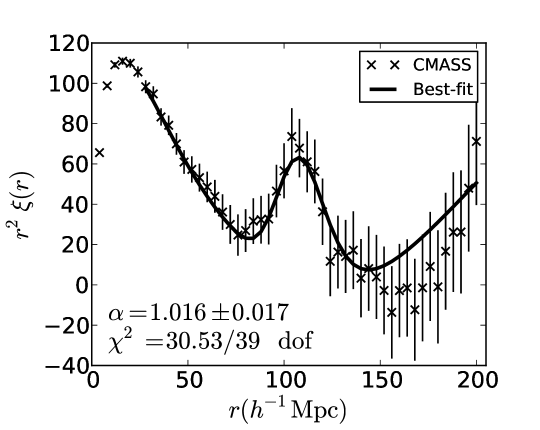
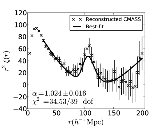
Fig. 3 plots the CMASS correlation functions before and after reconstruction, with the best-fit model (see below) overplotted. We estimate using the Landy & Szalay (1993) estimator
| (22) |
where , and are suitably normalised numbers of (weighted) data-data, data-random and random-random pairs. For the case of the reconstructed correlation function, the and pair counts in the numerator are replaced by and , where represents the shifted random particles. The errors are estimated by applying the same procedure to the mock catalogs and constructing the sample covariance matrix from the 600 realisations of . The average correlation function from the 600 mock catalogs is presented in Fig. 4. The errors in Fig. 3 are from the diagonal of the covariance matrix. We caution the reader that these errors are highly covariant, and assessing the significance requires analysing the full covariance matrix.
5.2 Fitting the correlation function
Our correlation function fits are based on the procedure described in Xu et al. (2012). We give a brief summary of the techniques here.
Our correlation function model is given by
| (23) |
where
| (24) |
and
| (25) |
In Eq. 24, the Gaussian term has been introduced to damp the oscillatory transform kernel at high- to induce better numerical convergence. The exact damping scale used in this term is not important, and we set , which is significantly below the scales of interest. The term is composed of nuisance parameters that help marginalize over the unmodeled broadband signal in the correlation function. Such broadband effects include redshift-space distortions, scale-dependent bias and any errors made in our assumption of the model cosmology. These effects may bias our measurement of the acoustic scale if not removed. is a multiplicative constant, allowing for an unknown large-scale bias. We use a template of the form
| (26) |
as given in Eisenstein et al. (2007b). Here, is the linear theory power spectrum and is the power spectrum with the BAO feature erased. The term is used to damp the acoustic oscillations in the linear theory power spectrum, serving to model the effects of non-linear structure growth. We fix in our fits to the pre-reconstruction correlation functions and in our fits to the post-reconstruction correlation functions. We normalise the template to the observed or mock correlation function being fit at , thereby ensuring that . These parameters were tuned on our mock catalogs, and we explicitly verify that are results are insensitive to these particular choices in Appendix B.2.
The scale dilation parameter defined in Eq. 21 captures our distance constraints; measures the relative position of the acoustic peak in the data versus the model, thereby characterising any observed shift. If , the acoustic peak is shifted towards smaller scales, and vice versa for .
We obtain the best-fit value of by computing the goodness-of-fit indicator at intervals of in the range , then identify the value of that gives the minimum and take this as our best-fit value. The as a function of is given by
| (27) |
where is the measured correlation function and is the best-fit model at each . is the sample covariance matrix, and we use a fitting range of . We therefore fit over 44 points using 5 parameters, leaving us with 39 degrees-of-freedom (dof). Assuming a multi-variate Gaussian distribution for the fitted data (this is tested and shown to be a good approximation in Manera et al. 2012), the probability distribution of is
| (28) |
The normalisation constant is determined by ensuring that the distribution integrates to 1. In calculating , we also impose a 15 per cent Gaussian prior on to suppress values of that correspond to the BAO being shifted to the edge of our fitting range at large scales. The sample variance is larger at these scales, and the fitting algorithm is afforded some flexibility to hide the acoustic peak within the larger errors.
The standard deviation of this probability distribution serves as an error estimate on our distance measurement. The standard deviation for the data and each individual mock catalog can be calculated as , where the moments of are
| (29) |
Note that refers to the mean of the distribution in this equation only.
In reference to the mocks, will denote the ensemble mean of the values measured from each individual mock, and will denote the median. The term “Quantiles” will denote the 16th/84th percentiles, which are approximately the 1 level if the distribution is Gaussian. The scatter predicted by these quantiles suffers less than the rms from the effects of extreme outliers.
5.3 Results
Using the procedure described in §5.2, we measure the shift in the acoustic scale from the CMASS DR9 data to be before reconstruction and after reconstruction. The quoted errors are the values measured from the probability distributions, . Plots of the data and corresponding best-fit models are shown in Fig. 3 for before (left) and after (right) reconstruction. We see that for CMASS DR9, reconstruction has not significantly improved our measurement of the acoustic scale. However, in the context of the mock catalogues, this result is not surprising.
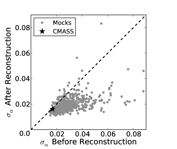
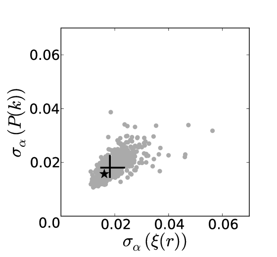
Fig. 5 shows the values measured from the mocks before reconstruction versus those measured after reconstruction from the correlation function fits. The CMASS DR9 point is overplotted as the black star and falls within the locus of mock points. However, we see that before reconstruction, our recovered for CMASS DR9 is much smaller than the mean expected from the mocks. For typical cases, reconstruction improves errors on , but if one has a “lucky” realisation that yields a low error to begin with, then reconstruction does not produce much improvement. The mock catalog comparison in Figure 5 shows that the BOSS DR9 data volume is just such a “lucky” realisation, with a strong and well defined acoustic peak, and it is therefore unsurprising that reconstruction does not reduce the error on .
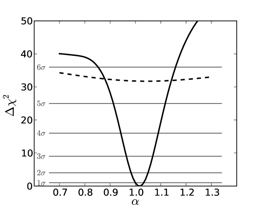
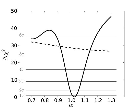
The BAO detection in the CMASS DR9 data is highly significant as illustrated in Fig. 6. Here we have plotted , where is the minimum that corresponds to the best-fit value of . The dashed line overplotted corresponds to fits to the data using a model without a BAO signature. This figure captures two tests of BAO significance: the first requires a comparison between the solid and dashed curves, and indicates how confident we are that the BAO feature exists in the CMASS DR9 data. The second uses the plateau height of the curve to indicate how confident we are that we have measured an acoustic feature.
The panel on the left corresponds to our pre-reconstruction results and the panel on the right corresponds to our post-reconstruction results. Before reconstruction, the minimum of the solid curve lies beyond a of 25 from the dashed curve, indicating that the BAO is detected in CMASS DR9 at greater than confidence. Local maxima are seen at greater than of 36 above the minimum, indicating that the data prefer our best-fit value of at more than . We see similar confidence levels post-reconstruction.
To verify the robustness of our techniques, we also measure the best-fit and for our 600 mock catalogues using our fiducial fitting and reconstruction parameters. We then repeat the same fitting with slightly altered models as well as on correlation functions computed from catalogues that were reconstructed using different parameters (bias, growth factor and smoothing scale). These fitting results are discussed in more detail in Appendix B and summarised in Table 5. The values in the table are computed after discarding the mocks with . Before reconstruction there were 10 such instances, and after reconstruction there was only 1 such instance. These large uncertainties in the measured indicate that the acoustic signature is weak in these realisations and is therefore not detected with high fidelity (see Xu et al. 2012 for a more detailed description of this approach). We find that regardless of fitting model parameters or reconstruction parameters, we always recover consistent measurements of the and . Hence, our fiducial model should be trusted to return reliable measurements of the acoustic scale.
Before reconstruction our mocks yield with an average error on any single realisation (i.e. the rms or standard deviation) of and a standard error on the mean of 0.001. The median is with quantiles of . After reconstruction, we obtain with average error on any single realisation of and standard error on the mean of 0.001. The median is with quantiles of . One can see that given the error on the mean, we detect a statistically significant shift in our measured mean from the true acoustic scale () expected in the mocks. This small systematic shift is discussed in more detail in Section 7.
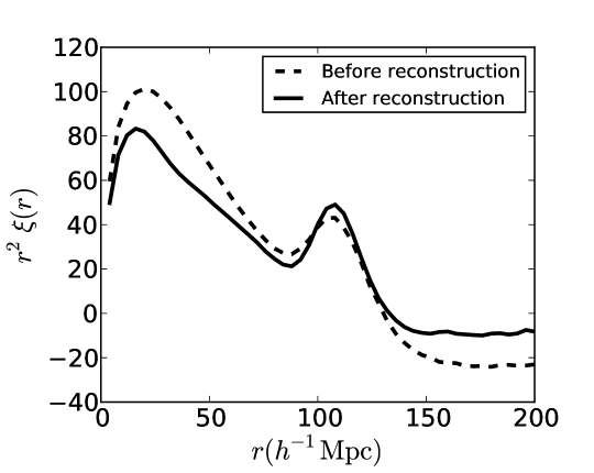
Most important, the average error on recovered from the mocks has decreased after reconstruction. This is illustrated in Fig. 5, where an overall improvement in is evident after reconstruction. The greatest improvements occur when the pre-reconstruction errors are the worst. The average decrease in is a factor of 1.54, which is equivalent to the effects of increasing the survey volume by a factor of 2.3. Therefore, reconstruction appears to significantly improve our ability to measure precisely, on average. This point is further illustrated in Fig. 4, where we have plotted the average mock correlation function before and after reconstruction. One can see the sharpening up of the acoustic peak, indicating the effectiveness of the reconstruction algorithm in partially removing the smearing of the BAO caused by non-linear structure growth. This improvement is what allows a more precise centroiding of the peak location. In fitting the average mock correlation function before and after reconstruction, we find , the damping of the BAO due to non-linear evolution, decreases from to . Beyond reducing the distance errors, reconstruction also makes our distance estimates more robust to parameter choices in our fitting algorithms and reduces the scatter between the distance estimates from the the correlation function and the power spectrum. We quantify these improvements further in following sections.
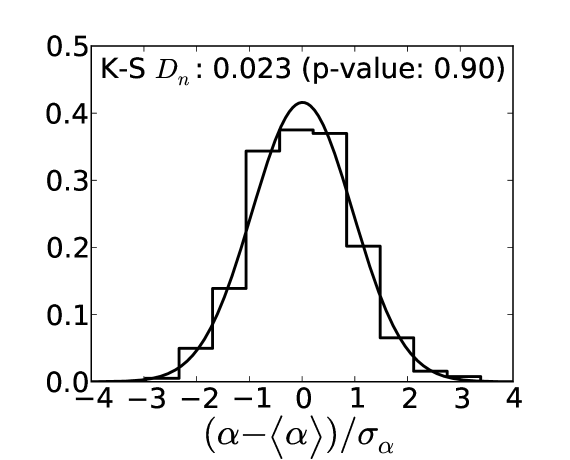
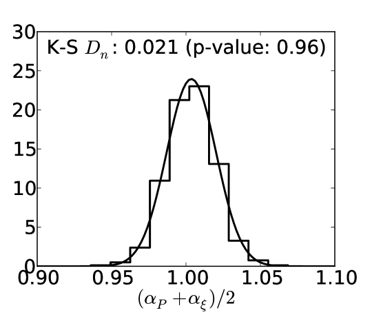
We next compare the observed scatter in the best-fit in the mocks to the estimated in each fit from the curve. In Fig. 7, we plot a histogram of from the mocks and compare the result to the unit normal distribution. We find excellent agreement; a Kolmogorov-Smirnov (K-S) test finds a high likelihood that the observed distribution is drawn from a unit normal. Hence the Gaussian probability distribution obtained from the statistic is an appropriate characterisation of the error on .
6 The Power Spectrum
6.1 Measuring the power spectrum
The power spectra recovered from the CMASS DR9 data are shown in Fig. 8 before (left) and after (right) reconstruction. The inset shows the oscillations in these data, calculated by dividing by a smooth model (see Section 6.2 for details). The effect of the reconstruction algorithm is clear - the large-scale power is decreased corresponding to the removal of RSD effects, with the small-scale power being further reduced by the reduction in non-linear power. These data represent the most accurate measurement of a redshift-space galaxy power spectrum ever obtained.
Power spectra were calculated using the Fourier method first developed by Feldman, Kaiser & Peacock (1994), as described in Percival et al. (2007b) and Reid et al. (2010). We work in redshift-space as if observed recession velocities solely arise from the Hubble expansion. As we focus on measuring angle-averaged Baryon Acoustic Oscillations, we do not convert from a galaxy density field to a halo density field as in Reid et al. (2010), or apply corrections for Finger-of-God effects. Given a weight for galaxy at location , the overdensity field can be written
| (30) |
where is a normalisation constant
| (31) |
and is the expected weighted distribution of galaxies at location in the absence of clustering, and is the galaxy density. The quantity is the standard Dirac- function. We do not apply luminosity-dependent weights (as applied by Percival et al. 2007b; Reid et al. 2010), as we are only interested in the BAO, and not the overall shape of the power spectrum.
We chose to model the expected distribution of galaxies using a random catalogue with points selected at the mean galaxy density , which is then weighted in a similar manner to the galaxies. The calculation of this catalogue was described in Section 3.8. The weights in the random catalogue are then renormalised, and compared with the weights applied to the galaxies so that , thereby matching the total weighted number density in galaxy and random catalogues.


Power spectra are calculated using a grid in a cubic box of length . This zero-pads the galaxies - the minimum and maximum galaxy redshifts of the sample correspond to distances of and , so the galaxies form an angular sector of a thick shell within this cube. The Nyquist frequency for the Fourier transform is approximately , which is significantly larger than the maximum frequency fitted of (see Section 6.2). The smoothing effect of the cloud-in-cell assignment used to locate galaxies on the grid (e.g. Hockney & Eastwood, 1981, chap. 5) is corrected, and shot-noise is subtracted following the assumption that galaxies form a Poisson sampling of the density field (see Feldman, Kaiser & Peacock 1994 for details). The power spectrum is then spherically averaged, leaving an estimate of the “redshift-space” power, binned into bins in of width .
6.2 Fitting the power spectrum
We fit the observed redshift-space power spectrum, calculated as described in Section 6, with a two component model comprising a smooth cubic spline multiplied by a model for the BAO, following the procedure developed by Percival et al. (2007a, c, 2010). The model power spectrum is given by
| (32) |
where is a smooth model that fits the overall shape of the power spectrum, and the BAO model , calculated for our fiducial cosmology, is scaled by the dilation parameter as defined in Eq. 21. The calculation of the BAO model is described in detail below. This scaling of the acoustic signal is identical to that used in the correlation function fits, although the differing non-linear prescriptions in (Eqns 23 & 32) means that the non-linear BAO damping is treated in a subtly different way.
Each power spectrum model to be fitted is convolved with the survey window function, giving our final model power spectrum to be compared with the data. The window function for this convolution is the normalised power in a Fourier transform of the weighted survey coverage, as defined by the random catalogue, and is calculated using the same Fourier procedure described in Section 6 (e.g. Percival et al. 2007c). This is then fitted to express the window function as a matrix relating the model power spectrum evaluated at wavenumbers, , equally spaced in , to the central wavenumbers of the observed bandpowers :
| (33) |
The final term arises because we estimate the average galaxy density from the sample, and is related to the integral constraint in the correlation function. In fact this term is smooth (as the power of the window function is smooth), and so can be absorbed into the smooth component of the fit, and we therefore do not explicitly include this term in our fits.
To model the overall shape of the galaxy clustering power spectrum we use a cubic spline (Press et al., 1992), with nine nodes fixed empirically at , and with , matching that adopted in Percival et al. (2007c, 2010). This model was tested in these papers, but we show in Section B.3 that it also provides an excellent fit to the overall shape of the DR9 CMASS mock catalogues, and that there is no evidence for deviations for the fits to the data.
To calculate our fiducial BAO model, we start with a linear matter power spectrum , calculated using CAMB (Lewis et al., 2000), which numerically solves the Boltzman equation describing the physical processes in the Universe before the baryon-drag epoch. We then evolve using the HALOFIT prescription (Smith et al., 2003), giving an approximation to the evolved power spectrum at the effective redshift of the survey. To extract the BAO, this power spectrum is fitted with a model as given by Eq. 32, where we adopt a fixed BAO model () calculated using the Eisenstein & Hu (1998) fitting formulae at the same fiducial cosmology. Dividing by the best-fit smooth power spectrum component from this fit produces our BAO model, which we denote .
We damp the acoustic oscillations to allow for non-linear effects
| (34) |
where the damping scale is a fitted parameter. We assume a Gaussian prior on with width , centred on for pre-reconstruction fits and for post-reconstruction fits, matching the average recovered values from fits to the 600 mock catalogs with no prior. The exact width of the prior is not important, but if we do not include such a prior, then the fit can become unstable with respect to local minima at extreme values.
We fit over scales : these limits are imposed because the BAO have effectively died out for , and scales are sensitive to observational systematics (Ross et al., 2012). We bin the measured power spectrum in bins of width , so 70 data points are included in the fits. The function depends on 9 free parameters, the amplitudes of the spline nodes. Thus, including and we fit to 11 parameters in total, and the fit has 59 degrees-of-freedom. Goodness of fit between model and data is calculated using the statistic. We consider intervals of in the range and, for each value of to be tested, we use the Powell routine (Press et al., 1992), starting from a series of widely separated start points, to find the spline node values and that result in the minimum value of .
For each power spectrum fitted, we have estimated the error on the best-fit value of by considering the interval and by integrating over the likelihood surface. These measurements are found to match extremely well for all of the fits, suggesting that the likelihood is well behaved around the minima. We also consider the distribution of best-fit recovered from the mock catalogues, as discussed in subsequent sections. For the results presented, in order to be consistent we adopted the procedure described in Section 5.2 to make measurements from the surfaces resulting from the power spectrum fits.
6.3 Results
We have measured the best-fit and using the procedure described in Section 6.2 for power spectra calculated from each of 600 mock catalogues and from the CMASS DR9 data, either before or after applying the reconstruction algorithm. The maximum likelihood solution for the dilation parameter from the full CMASS DR9 sample is before reconstruction and after reconstruction. Errors were determined from the moments of calculated by integrating the likelihood surface. The CMASS DR9 power spectra before (left) and after (right) reconstruction are plotted in Fig. 8, compared with the corresponding best-fit models. Before reconstruction, we find , while post-reconstruction this reduces to , with 59 degrees-of-freedom.
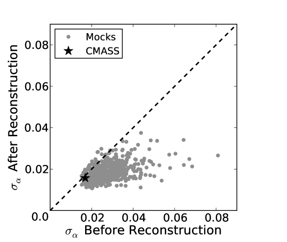
As for the correlation function measurements, we find that reconstruction does not significantly improve the measurement of the dilation parameter from the CMASS DR9 data. This is consistent with the results from the mock catalogs: we have measured and fitted power spectra calculated for all 600 mock catalogs, and Fig. 9 presents a scatter plot of the recovered errors before and after reconstruction. Although reconstruction improves the fit for the majority of the mock catalogs, there are a small number for which reconstruction increases the recovered error. Also, we see that improvement is more likely where the pre-reconstruction error is high, suggesting that variation in the error recovered from different catalogues is dominated by the “noise” that reconstruction is able to remove. In this plot, the star marks the result from the CMASS DR9 data, showing that the pre-reconstruction error recovered is significantly smaller than the mean expected from the mocks. Given this result, we should not be surprised that reconstruction only has a small effect on these data.
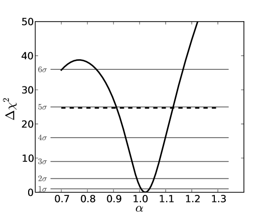
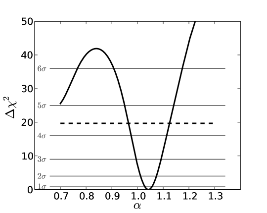
The BAO detection from the CMASS DR9 data is highly significant, with a difference between best-fit models with and without the BAO component being approximately before reconstruction, dropping slightly to post-reconstruction. The relatively small difference between significance before and after reconstruction matches the difference in discussed previously. The surfaces are shown in Fig. 10 before (left) and after (right) reconstruction. Low values of result in the BAO signal being moved to large scales where the cosmic variance error increases, which is why these models give comparatively good fits.
From the 600 mocks, pre-reconstruction we recover a mean value of the dilation parameter of , with average error on any single realisation of and standard error on the mean of . Post-reconstruction this reduces to , with average error on any single realisation of and standard error on the mean of . There is therefore evidence for a small systematic shift between the true value () for the mocks and the values recovered. A discussion of the systematic errors associated with our measurements is provided in Section 7. The decrease in mock rms post-reconstruction demonstrates the positive effect that reconstruction has on average. Note that when calculating the above mean recovered errors we excluded two mocks pre-reconstruction for which , where the BAO feature was not well recovered.
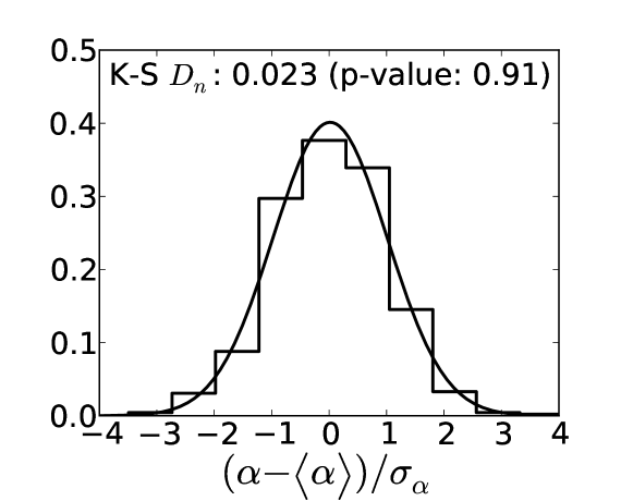
The mean values match perfectly with the standard deviation of the recovered values from the mocks, which give and pre- and post-reconstruction, indicating that the likelihood is extremely well behaved. This is not the case if the damping parameter is fixed at an incorrect value in the model to be fitted to the data: insufficient damping results in recovered errors that are too small with respect to the distribution, while over-damping leads to over-prediction of the errors. As in Section 5.3, we now test the nature of the distribution of recovered dilation parameters. Fig. 11 shows a histogram of compared with a standard Normal distribution. As is clearly evident, the data are extremely well matched to the Gaussian prediction; this is also indicated by the result of a K-S test.

Finally in this section we consider the average BAO signal recovered from the mock catalogues. For each mock, we divide the measured power spectrum by the smooth component of the best-fit solution convolved with the survey window function. The average of these values over all of the mocks is shown in Fig. 12 both before and after applying the reconstruction algorithm. The average effect of reconstruction is evident on small scales, with the BAO feature being enhanced by this algorithm. Fitting to the mocks without assuming a prior on gives average best-fit values of before reconstruction and following reconstruction, which shows the extent of the improvement afforded by this technique. Note that these are systematically different from the values of recovered from the correlation function fits, which results from the way in which the non-linear shape was fitted leading to different effective definitions of . In the fits, a multiplicative correction was used, while for , an additive correction was adopted: the fit required less damping as he additive correction already acts to damp the importance of the BAO component, while the multiplicative correction for afforded by the free shape is itself multiplied by the BAO model, and thus more damping is required.
7 The Distance to
| Before Reconstruction | |||
|---|---|---|---|
| After Reconstruction | |||
| Consensus | |||
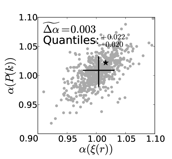
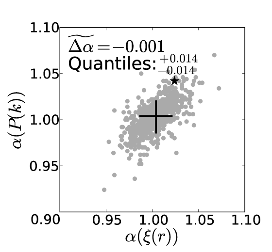
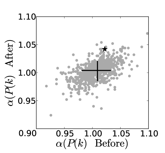

We now consider how to combine the power spectrum and correlation function analyses into one estimate for the cosmological distance scale. Before reconstruction, we find from the correlation function and from the power spectrum. After reconstruction, we find from the correlation function and from the power spectrum. These measurements are summarised in Table 6. These are small differences, but they approach 1 and hence demand a choice to be made.
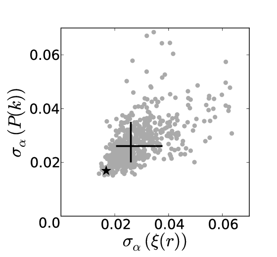
Importantly, our analysis of the mock catalogs shows that this level of scatter is not unusual. Fig. 13 compares the and errors recovered from and in our mocks. While the results are clearly correlated, there is a notable amount of scatter: about 2.1 per cent before reconstruction and 1.4 per cent after reconstruction, when one considers the 16–84 per cent quantile. The observed small difference in our CMASS measurements before reconstruction is unusually good; the larger difference after reconstruction is still common, only 1.2. Note that here we have not discarded any mocks with weak acoustic signals (i.e. ) as we are only comparing how and results fare against each other, and not examining details of the BAO. Fig. 14 compares before and after reconstruction for both estimators. Again we find that the shifts seem for the CMASS measurements and not unusual given the results from the mocks.
The mocks indicate that both estimators are reasonably unbiased: the mean recovered is shifted by only 0.4 per cent from the input value, and some of that shift is the actual physical shift of the acoustic scale due to non-linear gravity and galaxy clustering bias in the mocks (e.g., Crocce & Scoccimarro, 2008; Padmanabhan & White, 2009; Seo et al., 2010; Mehta et al., 2012). Furthermore, neither estimator performs notably better. As shown in the lower panels of Fig. 13, the errors formed from by the two estimators are comparable and correlate well on a mock-by-mock basis.
We therefore conclude that both the correlation function and power spectrum estimations of the acoustic scale are appropriate and unbiased, but that they include the noise from small scales and shot noise differently. Although the power spectrum and correlation function are Fourier transform partners in an ideal case, in practice this is not true: both functions are considered only over a limited domain and with binning.
Our choice for a consensus distance scale is therefore to average the two results. In our cosmological results, we use only the reconstructed case. Reconstruction is expected to improve the acoustic scale shifts from non-linear structure formation and galaxy clustering bias, and it does decrease the scatter in in our mock catalogs. The actual CMASS data show little change in recovered error on under reconstruction, but this is within the range of behaviours of the mocks and is not an argument for avoiding the method.
To estimate the error bars on the averaged estimator, we use the rms scatter of the results from the mocks for this estimator. Fig. 15 shows the distribution of average values from the mocks. The small K-S and p-value of 0.96 indicate that we are 96 per cent certain our measured values follow a Gaussian distribution. Since we expect our DR9 CMASS measurement to be Gaussian, using the rms of our mock values as our CMASS error estimate is valid. The mocks find a scatter of 1.7 per cent on the average , which is a small decrease from the scatter of 1.8 per cent on from and 1.9 per cent on from . This scatter is comparable to the 1.6 per cent error estimated from of the CMASS data from the fits in both and , which would be another reasonable approach to adopt an error. We note that since the averaging does produce a small improvement in errors, it is mildly conservative to neglect any improvement beyond the errors on the individual estimators.
We expect the systematic errors in this measurement to be much smaller than the statistical errors. The marginalization over broadband nuisance terms in the correlation function and over an arbitrary broadband spline in the power spectrum gives our template fits great stability to variations in the template or the possibility of systematic errors in the galaxy catalog. In Appendix B, we investigate a wide range of variations in the fitting methodologies and reconstruction choices, finding variations in of 0.2 per cent or less in all physically reasonable cases. It is more difficult to test the effects of systematics in the galaxy catalog, but if we ignore all of the corrections for the detected angular systematic variations and repeat the clustering analysis, the recovered value changes by only 0.1 per cent despite a notable increase in the large-scale power. This result is not surprising: systematic errors of this form tend to produce smooth changes in the power spectrum and hence are captured by the nuisance terms that we remove in our fitting methods.
Seo et al. (2008) and Xu et al. (2012) show that mild alterations in the cosmology used for the template in the fit changes the recovered at a negligible level, for variations consistent with WMAP, when averaged over a number of mock catalogues. Cosmologies more exotic than the usual cold dark matter families of course could open up more dramatic changes; in such cases, one should plan to repeat the fits both to the CMB and BAO data sets.
Our fitting to the mocks does return a value of that is 0.004 higher than the input value. As noted above, non-linear structure formation and galaxy bias do shift the acoustic scale. Seo et al. (2010) find shifts of order 0.002 from non-linear structure formation, while Mehta et al. (2011) finds a similar level from galaxy clustering bias. Perturbation theory calculations by Padmanabhan & White (2009) yield similar results. However, reconstruction has been found to remove these shifts, both in periodic box simulations (Seo et al., 2010; Mehta et al., 2011) and in SDSS-II mock catalogs (Padmanabhan et al., 2012a). It is possible that the BOSS DR9 survey geometry is not large and contiguous enough to remove the shifts in full, but it is also possible that the shift in the real data might be different than that in the mocks. As the shift is small, we have decided not to subtract it from our fitted values and instead to consider it as a small systematic uncertainty.
More exotic galaxy bias models could in principle add additional shifts. However, the only physically motivated model known that does couple to the acoustic scale is that of Tseliakhovich & Hirata (2010), in which relative velocities between the baryons and dark matter at high redshift modulate the ability of the smallest halos to trap gas. Whether this modulation will affect the properties of galaxies a million times more massive is speculative. Yoo et al. (2011) discuss how the imprint on the acoustic scale in galaxy clustering could be detected and removed using the three-point function, but we have not yet investigated this in the CMASS sample.
In summary, our consensus value for the acoustic scale fit is . Our estimates of systematic errors are significantly smaller than the statistical error and are negligible in quadrature. Our best value corresponds to a distance constraint of
| (35) |
We adopt this as our primary result and use it for all of our cosmological interpretations and comparisons to other work. For easy reference, the key values of are summarised in Table 2. For the fiducial sound horizon of 153.19 Mpc, Eq. (35) corresponds to Mpc.
8 The BAO distance ladder
8.1 Comparison to Previous BAO Measurements
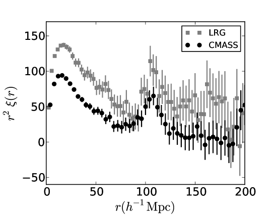
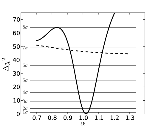


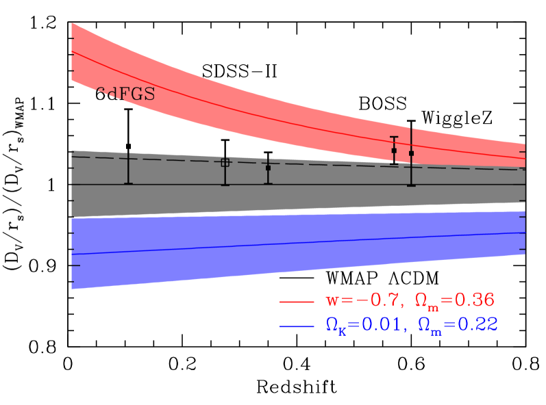
In the last few years, acoustic scale results have been obtained with a variety of data sets over a considerable range of redshift. We now focus on the comparison between our CMASS DR9 results and past work.
First, we compare the correlation function at from CMASS with that obtained at by the reconstruction analysis of SDSS-II LRGs presented in Padmanabhan et al. (2012a). Fig. 16 shows these two correlation functions as . The two samples involve different average masses of galaxies and redshifts, and hence have a different amplitude of clustering, leading to a vertical offset. Both correlation functions use our fiducial CDM cosmology. Given this choice of distance-redshift relation, one can see that the acoustic peaks are in excellent agreement.
Fig. 17 shows combined significance of the acoustic peak detection in . In combining the constraints on CMASS DR9 with the SDSS-II LRG DR7 data, we neglect the slight overlap in effective volumes when using these data in cosmological constraints. The LRG data fromPadmanabhan et al. (2012a) cover only the NGC which result in 2496 sq deg of overlapping area with CMASS over the redshift interval of . We find this is less than 9 per cent of the effective volume of our CMASS sample, and less than 5 per cent overlap with the LRG effective volume (fractionally less since the LRG DR7 data cover a larger area). This is consequently a good but not perfect assumption. Combining the two correlation functions assuming independence rejects models without acoustic oscillations at or 6.7 . Trying to place the acoustic peak at other nearby locations and particularly at smaller scales is rejected at 8 .
Fig. 18 repeats this comparison with the power spectrum from the SDSS-II LRG analysis presented in Reid et al. (2010) and Percival et al. (2010). This analysis did not use reconstruction, but one can see good agreement in the BAO and significant improvement in the error bars with the CMASS sample.
In Fig. 19, we plot constraints from measurements of the BAO from various spectroscopic samples. In addition to the SDSS-II LRG value at (Padmanabhan et al., 2012a) and the CMASS consensus result at , we also plot the constraint from the 6dF Galaxy Survey (6dFGS) (Beutler et al., 2011) and a constraint from the WiggleZ survey (Blake et al., 2011a). WiggleZ quotes BAO constraints in 3 redshift bins, but these separate constraints are weaker and there are significant correlations between the redshift bins. We choose here to plot their uncorrelated data points for . Each data point here is actually a constraint on , and we have multiplied by our fiducial to get a distance.
As described further in Mehta et al. (2012), the WMAP curve on this graph is a prediction, not a fit, assuming a flat CDM cosmology. For each value of and , one can predict a sound horizon, and the angular acoustic scale measured by WMAP plus the assumptions about spatial curvature and dark energy equation of state then provide a very precise breaking of the degeneracy between and and hence a unique . Taking the 1 range of and produces the grey band in Fig. 19. There is excellent agreement between all four BAO measurements and the WMAP CDM prediction.
Following Mehta et al. (2012), we divide the distance measurements by the best-fit WMAP prediction (, ) to yield Fig. 20. Focusing first on the data points and the grey CDM region, the data points are consistent with the WMAP prediction, but tend to lie closer to the 1 upward trend in WMAP, toward higher . In other words, if the WMAP value for were 1 higher, then all of the BAO points would be in superb consistency with themselves and the CMB under a flat CDM cosmology; recall that the swath of grey models is a nearly one-parameter family so all redshifts move together. We also include here the BAO measurement from Percival et al. (2010). Because of the overlap in sample with the LRG analysis of Padmanabhan et al. (2012a), we use a different symbol for this measurement. The correlation function analysis from Kazin et al. (2010) gives similar agreement. The CMASS BAO value is in perfect agreement with the WiggleZ measurement (Blake et al., 2011a). The WiggleZ acoustic scale error is 3.9 per cent (using their constraint on ), so the CMASS DR9 error of 1.7 per cent represents a 5-fold improvement in the variance.
Also shown in Fig. 20 is how the WMAP prediction changes as one varies the assumptions about dark energy and spatial curvature. For any specific choice of and , WMAP predicts a narrow region set by the range of and . Here we present the case of with a cosmological constant and a flat Universe with ; both produce large differences from the observations.
There have also been BAO measurements at using photometric samples (Padmanabhan et al., 2007; Carnero et al., 2012; Seo et al., 2012). These measure the angular diameter distance rather than . Carnero et al. (2012) measured at using the angular correlation function (Crocce et al., 2011) of SDSS DR7 imaging data (Abazajian et al., 2009). Seo et al. (2012) on the other hand measured at using the angular power spectrum (Ho et al., 2012) of the SDSS-III DR8 imaging data (Aihara et al., 2011) 777The DR8 measurement used square degrees of the sky that includes the coverage of the CMASS DR9 sample. Therefore the overlap in volume between the two samples is approximately 30 per cent.. Despite the different estimators of two-point statistics used, both results consistently show a larger distance scale than the prediction of the WMAP best-fit by and , respectively. To compare these values with spectroscopic measurements, we correct the difference between and using the calculated from the fiducial cosmology, while translating the percentage error on to be the percentage error on . The deviation from the WMAP prediction will be reduced due to using the fiducial during this transformation; the correction yields and , respectively. Extrapolating these values from to assuming the fiducial cosmology gives for Carnero et al. (2012) and for Seo et al. (2012). Therefore the photometric BAO measurements show an excellent agreement with from the CMASS measurement. It is clear that these photometric BAO measurements also fall into the general upward trend relative to the WMAP prediction.
Similarly, there have been spectroscopic BAO measurements that attempt to separate the line-of-sight and transverse clustering so as to measure and separately (Okumura et al., 2008; Chuang & Wang, 2011). These measurements are at lower redshift and hence not directly comparable to our CMASS result. However, the agreement in the recovered cosmological parameters is good.
In summary, a precise view of the Hubble diagram from baryon acoustic oscillations over the range is taking shape. These measurements appear highly consistent with the standard cosmological model.
8.2 Comparison to Supernova and Direct Measurements
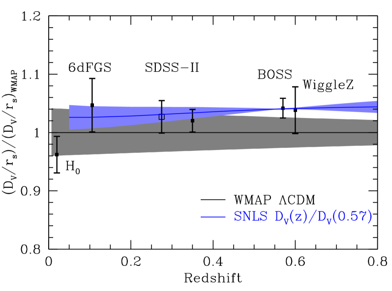
We next offer further comparisons to the distance-redshift relation from Type Ia supernovae and direct measurements. Type Ia supernovae can be used to measure relative luminosity distances. We use the 3-year Supernova Legacy Survey (SNLS3) results from Conley et al. (2011), including their systematic error treatment. Comparing the supernova distance-redshift relation to that of the BAO requires some procedure to bin the individual data points or to fit a model (see Lampeitl et al. 2010 for a discussion of possible procedures). Due to the systematic errors and the absolute distance offset, combining the supernova data into redshift bins would necessarily yield correlated results. Moreover, the supernovae results constrain the luminosity distance , not the measured by the BAO. requires as well, which is related to a derivative of , with a mild dependence on spatial curvature. The need for this derivative recommends fitting a model instead of binning.
We opt to fit a parametric model. We run Markov Chain Monte Carlo (described in the next section) for a model space including spatial curvature and an equation of state . We use CMB data from WMAP in addition to the SNLS3 data; we opt to include CMB measurements so that the dependence on spatial curvature remains mild. CMB data alone would have 3 dimensions of significant degeneracies in this parameter space; the supernova data will attempt to break these degeneracies. We then use the Markov Chain to infer the constraints on ratios of to . This tells us what the supernova distance-redshift relation predicts for the ratio between two BAO measurements, subject to the regularisation of the supernova data implied by the parametric cosmological model that we have chosen. In effect, we have fit a three-parameter distance-redshift relation to the supernova data and then used this to infer from the observed distance moduli. As a technical note, these results will differ slightly from those from MCMC that combine BAO and SNe data, because the BAO data will limit the exploration of the distance-redshift degeneracy space.
Comparing to , we find that the supernovae measure , a 1.0 per cent inference. From the CMASS measurement of , this predicts , where the first error arrises from the CMASS error and the second error is due to the error in the supernova propagation. This prediction can be compared to the Padmanabhan et al. (2012a) measurement from SDSS-II LRG of . Hence, the ratio of these two BAO measurements agrees well with the supernova data.
Similarly, at , we find that the supernovae measure , a 1.9 per cent inference. The combination with the CMASS data would then predict , following the notation from the previous paragraph. This can be compared to the 6dFGS measurement of , where we have scaled from to . Again, the ratio of the BAO measurements agrees well with the supernova distance scale.
We present these results graphically in Fig. 21. Here, we normalise the from the Markov Chain at and consider the mean and 1 range explored by the chain. Of course, one might have chosen to normalise at another redshift; this version presents how well the CMASS BAO data can be transferred to other redshifts. One can see the excellent agreement with all of the other BAO results. One also sees that the supernova relative distance scale is still more constraining than the BAO relative distance scale, by a factor of order 2-3. Of course, the supernovae do not provide an absolute distance scale; this plot is indicating only their constraint on the slope of the distance-redshift relation. In the future, we many wish to combine SNe and BAO distances to further constrain the reciprocity, or distance-duality, relation which is a generic prediction of any theory of gravity where photons follow null geodesics (Bassett & Kunz, 2004; Lampeitl et al., 2010).
Finally, considering the constraint on the Hubble constant, the supernovae predict a tight relation between and . We quote this quantity as with a 2.3 per cent error. Using this result, the CMASS BAO data with a sound horizon given by the fiducial cosmological model predicts km/s/Mpc, with 1.7 per cent error from the calibration and 2.3 per cent error from the supernova transfer to . This value is in mild tension with the direct measurement of km/s/Mpc using the NGC 4258 maser and HST near-IR observations of Cepheid variable stars (Riess et al., 2011). Fig. 21 plots this measurement, but we remind readers that the placement of this point assumes the fiducial value of , which creates a 1 per cent uncertainty not included in the errors. We will quantify this point further in the next section, using a full Markov Chain.
9 Cosmological parameters
| Dataset Name | Description | References |
|---|---|---|
| CMB | WMAP7 data | Komatsu et al. (2011) |
| LRG | SDSS-II Luminous Red Galaxies | Padmanabhan et al. (2012a) |
| 6dFGRS | 6dF Galaxy Redshift Survey sample | Beutler et al. (2011) |
| CMASS | SDSS-III Data Release 9 Constant Mass Sample | This paper |
| SN | 3-year Supernova Legacy Survey compilation (SNLS3) | Conley et al. (2011) |
| H0 | Direct Hubble Constant Measurement | Riess et al. (2011) |
| Cosmological Model | Data Sets1 | ||||||
| km/s/Mpc | |||||||
| CDM | CMB | 0.1341(56) | 0.268(29) | 71.0(26) | |||
| CDM | CMB+CMASS | 0.1392(36) | 0.298(17) | 68.4(13) | |||
| CDM | CMB+LRG | 0.1362(33) | 0.280(14) | 69.8(12) | |||
| CDM | CMB+LRG+CMASS | 0.1384(31) | 0.293(12) | 68.8(10) | |||
| CDM | CMB+LRG+CMASS+6dF | 0.1384(31) | 0.293(12) | 68.7(10) | |||
| CDM | CMB+LRG+CMASS+SN | 0.1373(30) | 0.287(11) | 69.2(10) | |||
| CDM | CMB+LRG+CMASS+SN+6dF | 0.1373(30) | 0.288(11) | 69.1(10) | |||
| oCDM | CMB | 0.1344(55) | 0.423(175) | 60.0(123) | -0.039(44) | ||
| oCDM | CMB+CMASS | 0.1340(53) | 0.299(16) | 67.0(15) | -0.008(5) | ||
| oCDM | CMB+LRG | 0.1333(53) | 0.278(15) | 69.3(16) | -0.004(5) | ||
| oCDM | CMB+LRG+CMASS | 0.1336(51) | 0.288(12) | 68.1(11) | -0.006(5) | ||
| oCDM | CMB+LRG+CMASS+6dF | 0.1336(50) | 0.288(12) | 68.1(11) | -0.006(5) | ||
| oCDM | CMB+LRG+CMASS+SN | 0.1322(51) | 0.284(12) | 68.3(12) | -0.006(5) | ||
| oCDM | CMB+LRG+CMASS+SN+6dF | 0.1321(50) | 0.284(12) | 68.2(11) | -0.007(5) | ||
| CDM | CMB | 0.1342(58) | 0.263(105) | 75.4(138) | -1.12(41) | ||
| CDM | CMB+CMASS | 0.1358(59) | 0.323(43) | 65.4(60) | -0.87(24) | ||
| CDM | CMB+LRG | 0.1349(57) | 0.285(25) | 69.0(39) | -0.97(17) | ||
| CDM | CMB+LRG+CMASS | 0.1370(58) | 0.294(27) | 68.6(44) | -0.99(21) | ||
| CDM | CMB+LRG+CMASS+6dF | 0.1363(51) | 0.298(20) | 67.8(31) | -0.95(15) | ||
| CDM | CMB+LRG+CMASS+SN | 0.1399(37) | 0.280(13) | 70.8(18) | -1.09(8) | ||
| CDM | CMB+LRG+CMASS+SN+6dF | 0.1396(37) | 0.282(13) | 70.4(17) | -1.08(8) | ||
| oCDM | CMB+LRG+CMASS | 0.1345(53) | 0.250(42) | 74.1(70) | -0.008(5) | -1.31(34) | |
| oCDM | CMB+LRG+CMASS+6dF | 0.1334(52) | 0.271(31) | 70.5(43) | -0.007(6) | -1.14(23) | |
| oCDM | CMB+CMASS+SN | 0.1338(53) | 0.280(17) | 69.2(21) | -0.009(5) | -1.10(8) | |
| oCDM | CMB+LRG+CMASS+SN | 0.1337(53) | 0.275(14) | 69.8(18) | -0.007(5) | -1.09(8) | |
| oCDM | CMB+LRG+CMASS+SN+6dF | 0.1333(52) | 0.276(13) | 69.6(17) | -0.008(5) | -1.09(8) | |
| CDM | CMB+LRG+CMASS | 0.1377(58) | 0.282(52) | 70.7(68) | -1.11(51) | 0.18(122)* | |
| CDM | CMB+LRG+CMASS+6dF | 0.1369(55) | 0.292(41) | 68.9(48) | -1.02(42) | 0.44(113)* | |
| CDM | CMB+CMASS+SN | 0.1389(62) | 0.281(17) | 70.3(23) | -1.07(16) | -0.85(96)* | |
| CDM | CMB+LRG+CMASS+SN | 0.1392(59) | 0.280(14) | 70.6(19) | -1.08(15) | 0.10(87) | |
| CDM | CMB+LRG+CMASS+SN+6dF | 0.1385(58) | 0.281(14) | 70.2(17) | -1.08(15) | 0.08(81) | |
| oCDM | CMB+LRG+CMASS | 0.1347(54) | 0.263(54) | 72.7(79) | -0.009(6) | -1.13(54) | -0.70(139)* |
| oCDM | CMB+LRG+CMASS+6dF | 0.1341(53) | 0.284(40) | 69.2(50) | -0.009(7) | -0.93(41) | -0.93(130)* |
| oCDM | CMB+CMASS+SN | 0.1344(54) | 0.280(17) | 69.5(21) | -0.012(6) | -0.91(17) | -1.31(102)* |
| oCDM | CMB+LRG+CMASS+SN | 0.1348(53) | 0.277(14) | 69.8(18) | -0.012(5) | -0.89(16) | -1.44(93)* |
| oCDM | CMB+LRG+CMASS+SN+6dF | 0.1343(52) | 0.278(14) | 69.5(17) | -0.012(5) | -0.88(15) | -1.40(94)* |
| oCDM | CMB+LRG+CMASS+SN+H0 | 0.1364(51) | 0.270(12) | 71.1(15) | -0.010(5) | -0.93(16) | -1.46(95)* |
| oCDM | CMB+LRG+CMASS+SN+H0+6dF | 0.1359(50) | 0.270(12) | 70.8(14) | -0.010(5) | -0.93(16) | -1.39(96)* |
1 The CMB+LRG values are taken from Mehta et al. (2012). * Datasets allow chains to explore parameter space outside the prior of .
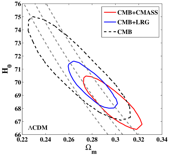
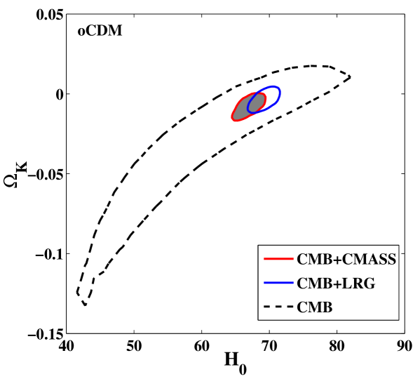
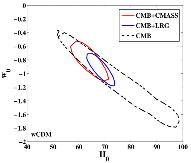
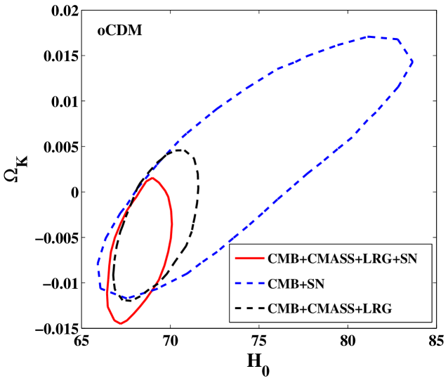
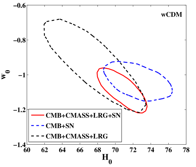
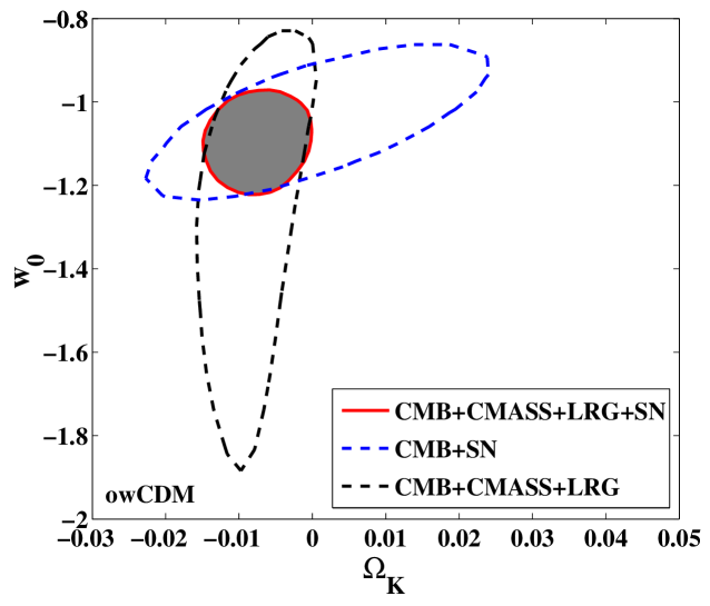
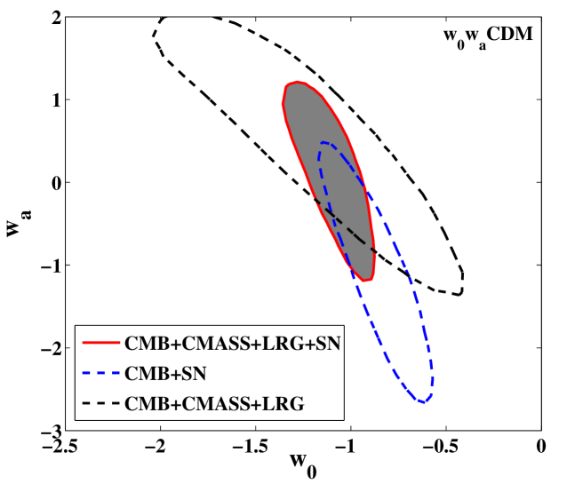
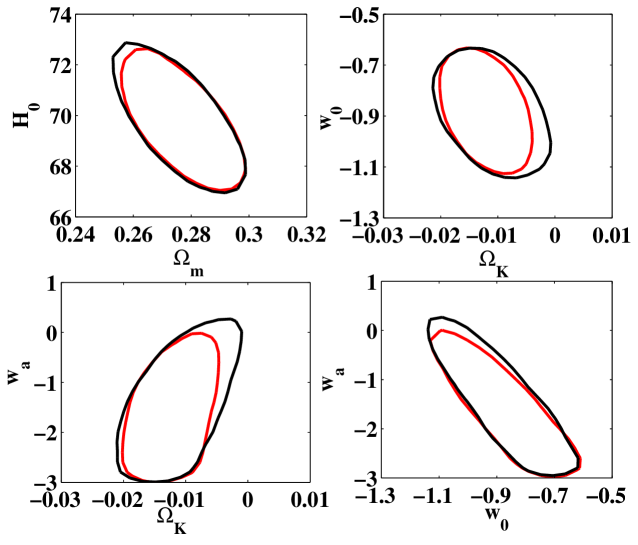
To explore the implications of these results for the values of cosmological parameters, we consider the standard CDM parametrisation of the baryon and matter densities , the primordial power spectrum slope , the optical depth to reionization , the Hubble constant and the amplitude of matter clustering . We also examine models with a non-zero curvature as well as models where the dark energy differs from a cosmological constant with an equation of state parameterised by (Chevallier & Polarski, 2001; Linder, 2003), where is the scale factor.
We follow the methodology in Mehta et al. (2012), using the CosmoMC (Lewis & Bridle, 2002) Markov Chain Monte Carlo sampler to map the posterior distributions of these parameters. Our BAO distance constraints are parameterised as described above as a measurement on at ; we augment these with the measurement from Padmanabhan et al. (2012a) as well as the 6dF measurement at (Beutler et al., 2011). These measurements have very little overlap in redshift and cover different angular patches, and we treat them independently. We do not include the WiggleZ measurements (Blake et al., 2011a, b) given the significant overlap with the sample presented here. However, as discussed in the previous section, the WiggleZ measurements agree very well with the distances derived in this work. In addition to these BAO measurements, we include observations of the temperature and polarization fluctuations in the cosmic microwave background (CMB) by the WMAP satellite (Komatsu et al., 2011), as well as measurements of the expansion history by the 3-year Supernova Legacy Survey (Conley et al., 2011) and local measurements of the Hubble constant by Riess et al. (2011). We summarise the data sets used in Table 3.
We summarise our estimated cosmological parameters and their uncertainties for different assumptions about the background cosmology in Table 4. The discussion below highlights particular cross-sections through this space of models and parameters, focusing on comparisons between the LRG and CMASS samples as well as comparisons between the cosmological constraints from the BAO and supernova data.
The most restricted model we consider (denoted CDM) is a CDM cosmology with no spatial curvature; the dark energy is assumed to be a cosmological constant with . As is clear from Fig. 22, this model is already highly constrained by the CMB through a combination of constraints on the physical matter density and the distance to the last scattering surface. However, the current WMAP data cannot fully separate and , leading to an uncertainty in both of these measurements along the direction of constant , where (Percival et al., 2002). Adding a single low redshift distance measurement, from either the LRG or CMASS data, significantly reduces this uncertainty. The similar errors of the two BAO distances lead to similar constraints on : 1.2 kms-1Mpc-1 for the LRG sample and 1.3 kms-1Mpc-1 for the CMASS sample (a 1.7 per cent measurement). Combining these reduces this error to 1.0 kms-1Mpc-1 (a 1.4 per cent measurement), a reduction by (Table 4).
Allowing the curvature or (for a constant equation of state) to vary (denoted CDM and CDM respectively) opens up a degeneracy in the plane when only the CMB data are considered (Figs. 23 and 24). This degeneracy is broken by the introduction of a single distance measurement, as one might have expected from Fig. 20. The larger degeneracy in and the subsequently tighter constraints from the BAO measurements compared to results from the different redshifts at which curvature and dark energy become important. The BAO and CMB measurements are connected through the sound horizon and curvature has the dominant effect on this lever arm. This effect is visually apparent in Fig. 20, where the effect of curvature is mostly an offset in the distance-redshift relation (over the redshifts for which we are sensitive), while changing results in a non-trivial change to the shape of the distance redshift relation. This result also explains the difference in the improvement when the LRG and CMASS samples are combined. The two samples do not have a wide enough lever arm to improve the constraints on in the CDM case. By contrast, for the CDM case, the errors in drop by per cent from the LRG only case.
For both these cosmological models, one can also compare the constraints from the SN data with those from the BAO data as shown in Figs. 25 and 26. The qualitative difference between the SN and BAO distance ladders is that while the SN data are a regular distance ladder, building out from low redshift to high redshift, the BAO are an “inverse” distance ladder, calibrated at the CMB and extending down to low redshift. The SN therefore only weakly constrain the curvature (Fig. 25) and are more sensitive to , with the reverse being true for BAO. This effect is reflected in Figs. 25 and 26. The constraints on curvature are significantly improved by the BAO data, and they do not improve significantly upon the addition of the SN data. For the CDM case, while the BAO measurements have lower constraining power, their different redshift dependence gives them a different degeneracy direction to the SN, resulting in improved constraints. These trends are repeated when we consider two parameter models of the expansion history: CDM (Fig. 27) and CDM (Fig. 28), with the error ellipses being more orthogonal when the curvature is allowed to vary.
None of the individual probes are currently sufficiently sensitive to constrain the combination of , and . We therefore combine the SN and BAO data to obtain constraints on these models (Fig. 29). This cosmological model is also the one recommended by the Dark Energy Task Force (Albrecht et al., 2006) as the baseline to compare different dark energy experiments. They recommend using the inverse of the area of the 95 per cent error ellipse in the plane as a “Figure of Merit” (FoM) for the experiment. Our results (CMB+LRG+SN+CMASS) yield a FoM of 14.4, compared to a FoM of 11.5 (CMB+LRG+SN) reported by Mehta et al. (2012); the improvement driven by the inclusion of the higher precision BOSS measurement is clear.
Finally, as was discussed extensively in Mehta et al. (2012), the combination of the SN and BAO distances allows one to transfer the CMB distance scale down to the local Universe and constrain . Fig. 30 demonstrates that the resulting value of is robust to changes in assumed cosmological model. While the difference between the inferred value of from these data and the direct measurement of Riess et al. (2011) is not statistically significant in these data (), they may be brought into better agreement by adding an additional relativistic energy density component equivalent to neutrino species, instead of the canonical (see e.g. Mehta et al. 2012 for more details on the mechanism). Improvements in both data sets in the future will elucidate if the introduction of new physics is warranted or if the explanation is more mundane.
10 Discussion
We have presented the first constraints on cosmology and the distance scale from the Data Release 9 CMASS galaxy sample of the Baryon Oscillation Spectroscopic Survey. Our results are based on accurate 3D positions of massive galaxies covering 3275 sq. deg. with an effective redshift . This is the largest sample of the Universe ever surveyed at this high density and the derived BAO constraints are the most accurate determination of the distance scale within the crucial redshift range where the expansion of the Universe begins to accelerate.
The large survey volume and high sampling density of the CMASS galaxies allow the detection of the acoustic oscillations predicted by theories of the early Universe at very high significance (). The acoustic signature is seen both as a clear peak in the correlation function and a series of “wiggles” in the power spectrum. The measures are highly consistent, and we use both statistics in our final results. We determine the statistical significance of our measurements using a large number of mock catalogs based on second order Lagrangian perturbation theory (Manera et al., 2012), and test the covariance matrices so derived with two analytic methods. Our analysis of the mock catalogs shows that our measurements and their errors are not at all unusual, and would be expected given our sampling if the underlying cosmology were of the CDM family. Applying reconstruction (Eisenstein et al., 2007a) to the data does not significantly improve our measurement of the acoustic signature, which is to be expected based on comparison to mock catalogs since the pre-reconstruction error in the CMASS DR9 data is smaller than for a “typical” realisation.
We obtain a distance measurement from the power spectrum and correlation function by fitting the acoustic feature to an appropriately scaled template, while marginalising over variations in the broad-band shape. Our results are very robust to the procedure employed to marginalize over broad-band power, and indeed the configuration- and Fourier-space fits provide consistent constraints even though the template form and procedure are quite different. The scale parameter, , relates to the value in a fiducial cosmology. Since we use angle-averaged statistics in this work, the relevant distance measure is , and it is measured relative to the sound horizon, . Since the correlation function and power spectrum include noise from small-scales and shot-noise differently, we average the two determinations to obtain our consensus result on the distance to , , where we use the scatter in the mock catalogs as an estimate of the error ( per cent) on this average.
Reid et al. (2012) and Sanchez et al. (2012) use the correlation function over a wide range of scales to constrain cosmological parameters. We find excellent agreement between their results and the pure-BAO measurement described here, despite slightly different choices of binning, fit range, etc. This demonstrates that the distance information is dominated by the sharp acoustic feature rather than the broad-band power (which we have explicitly marginalised over in our analysis).
The BOSS result can be combined with other BAO measurements to form an “inverse distance ladder” which tightly constrains the expansion rate from to . The acoustic signature measured in BOSS is in excellent agreement with earlier SDSS results (Percival et al., 2010; Padmanabhan et al., 2012a), and the distance to is in almost perfect agreement with that inferred by WiggleZ (Blake et al., 2011a). In general the independent BAO results are all consistent with the same underlying (flat, CDM) cosmology. Even with only a fraction of the survey completed, the BOSS constraint is already the tightest distance constraint in the ladder ( per cent), with an errorbar 2.3 times smaller at than the combined, earlier WiggleZ measurements (Blake et al., 2011a). The BAO distance ladder suggests a slightly larger distance scale than the best-fit to the 7-year WMAP data, lying closer to the upper limit in WMAP toward higher . With this slightly higher value of , the BAO measurements are in superb agreement with each other and the CMB within the context of a flat CDM cosmology. While SNe do not provide an absolute distance, the relative distance scale inferred from SNLS SNe data is in good agreement with that inferred from BAO.
BOSS continues to amass data, and we expect these constraints to tighten significantly, as data will be collected through mid-2014.
11 Acknowledgements
WJP is grateful for support from the UK Science and Technology Facilities Research Council, the Leverhulme Trust, and the European Research Council. AJR is grateful to the UK Science and Technology Facilities Council for financial support through the grant ST/I001204/1. CGS acknowledges funding from project AYA2010-21766-C03-02 of the Spanish Ministry of Science and Innovation (MICINN). DJE, XX, and KM were supported by NSF grant AST-0707725 and NASA grant NNX07AH11G. SH and DJS are supported by the US Department of Energy’s Office of High Energy Physics (DE-AC02-05CH11231). NP and AJC are partially supported by NASA grant NNX11AF43G. FP acknowledges support from the Spanish MICINN’s Consolider grant MultiDark CSD2009-00064. MAS was supported by NSF grant AST-0707266. MECS was supported by the NSF under Award No. AST-0901965.
Funding for SDSS-III has been provided by the Alfred P. Sloan Foundation, the Participating Institutions, the National Science Foundation, and the U.S. Department of Energy Office of Science. The SDSS-III web site is http://www.sdss3.org/.
SDSS-III is managed by the Astrophysical Research Consortium for the Participating Institutions of the SDSS-III Collaboration including the University of Arizona, the Brazilian Participation Group, Brookhaven National Laboratory, University of Cambridge, Carnegie Mellon University, University of Florida, the French Participation Group, the German Participation Group, Harvard University, the Instituto de Astrofisica de Canarias, the Michigan State/Notre Dame/JINA Participation Group, Johns Hopkins University, Lawrence Berkeley National Laboratory, Max Planck Institute for Astrophysics, Max Planck Institute for Extraterrestrial Physics, New Mexico State University, New York University, Ohio State University, Pennsylvania State University, University of Portsmouth, Princeton University, the Spanish Participation Group, University of Tokyo, University of Utah, Vanderbilt University, University of Virginia, University of Washington, and Yale University.
We acknowledge the use of the Legacy Archive for Microwave Background Data Analysis (LAMBDA). Support for LAMBDA is provided by the NASA Office of Space Science.
The reconstruction computations were supported by facilities and staff of the Yale University Faculty of Arts and Sciences High Performance Computing Center. The MCMC computations in this paper were run on the Odyssey cluster supported by the FAS Science Division Research Computing Group at Harvard University.
Catalogue construction, power spectrum calculations, and fitting made use of the facilities and staff of the UK Sciama High Performance Computing cluster supported by the ICG, SEPNet and the University of Portsmouth, and the COSMOS/Universe supercomputer, a UK-CCC facility supported by HEFCE and STFC in cooperation with CGI/Intel.
References
- Abazajian et al. (2009) Abazajian, K. N., et al., 2009, ApJS, 182, 543 (DR7)
- Ade et al. (2011) Ade P., et al., 2011, A&A, in press [arxiv:1101.2022]
- Aihara et al. (2011) Aihara, H., Allende Prieto, C., An, D., et al. 2011, ApjS, 193, 29
- Alcock & Paczynski (1979) Alcock C., Paczynski B., 1979, Nature, 281, 358.
- Albrecht et al. (2006) Albrecht A., et al., 2006, astro, [arXiv:astro-ph/0609591]
- Bassett & Kunz (2004) Bassett B., Kunz M., 2004, PRD, 69, 1012305
- Beutler et al. (2011) Beutler F., et al., 2011, MNRAS, 416, 3017
- Blake et al. (2007) Blake C., Collister A., Bridle S., Lahav O., 2007, MNRAS, 374, 1527
- Blake et al. (2011a) Blake C., et al., 2011a, MNRAS, 415, 1707
- Blake et al. (2011b) Blake C., et al., 2011b, MNRAS, 415, 2892
- Blanton et al. (2003) Blanton M., et al., 2003, AJ, 125, 2276
- Cabré & Gaztañaga (2011) Cabré, A., & Gaztañaga, E. 2011, MNRAS, 412, L98
- Cannon et al. (2006) Cannon, R., et al., 2006, MNRAS, 372, 425
- Carnero et al. (2012) Carnero, A., et al., 2012, MNRAS, 419, 1689
- Chevallier & Polarski (2001) Chevallier M., Polarski D., 2001, Int. J. Mod. Phys. D 10, 213
- Chuang & Wang (2011) Chuang, C.-H., Wang, Y., 2011, [arXiv:1102:2251]
- Cole et al. (2005) Cole S., et al., 2005, MNRAS, 362, 505
- Colless et al. (2003) Colless M., et al., 2003, [astro-ph/0306581]
- Conley et al. (2011) Conley A., et al., 2011, ApJS, 192, 1
- Crocce & Scoccimarro (2008) Crocce, M., & Scoccimarro, R., 2008, Phys. Rev. D, 77, 023533
- Crocce et al. (2011) Crocce, M., et al., 2011, MNRAS, 417, 2577
- Dawson et al. (2012) Dawson K., et al., 2012, in preparation.
- de Putter et al. (2012) de Putter R., et al., 2012 [arxiv:111.6596]
- Doi et al. (2010) Doi M., et al., 2010, AJ, 139, 1628
- Doroshkevich et al. (1978) Doroshkevich A.G., Zel’dovich Ya.B., Sunyaev R.A., 1978 Soviet Astronomy, 22, 523
- Drinkwater et al (2010) Drinkwater M., et al., 2010, MNRAS, 401, 1429
- Eisenstein & Hu (1998) Eisenstein D.J., Hu W., 1998, ApJ, 496, 605
- Eisenstein et al. (1998) Eisenstein D.J., Hu W., Tegmark M., 1998, ApJ, 504, L57
- Eisenstein et al. (2001) Eisenstein D.J., et al., 2001, AJ, 122, 2267
- Eisenstein (2003) Eisenstein D.J., 2003, in Wide-field multi-object spectroscopy, ASP Conference Series, ed. A. Dey.
- Eisenstein et al. (2005) Eisenstein D.J., et al., 2005, ApJ, 633, 560
- Eisenstein et al. (2007a) Eisenstein D. J., Seo H.-J., Sirko E., Spergel D. N., 2007a, ApJ, 664, 675
- Eisenstein et al. (2007b) Eisenstein D.J., Seo H.-J., White M., 2007b, ApJ, 664, 660
- Eisenstein (2008) Eisenstein D.J., Bennett C.L., 2008, Physics Today, April, p. 44
- Eisenstein et al. (2011) Eisenstein D.J., et al., 2011, AJ, 142, 72 [arxiv:1101.1529]
- Feldman, Kaiser & Peacock (1994) Feldman H.A., Kaiser N., Peacock J.A., 1994, ApJ, 426, 23
- Fukugita et al. (1996) Fukugita M., et al., 1996, AJ, 111, 1748
- Gaztanaga, Cabre & Hui (2009) Gaztanaga E., Cabre A., Hui L., 2009, MNRAS, 399, 1663
- Glazebrook & Blake (2005) Glazebrook K., Blake C., 2005, Astrophys. J., 631, 1
- Górski et al. (2005) Górski, K. M., Hivon, E., Banday, A. J., Wandelt, B. D., Hansen, F. K., Reinecke, M., & Bartelmann, M. 2005, ApJ, 622, 759
- Gramann (1993) Gramann, M. 1993, ApJ, 405, 449
- Guo et al. (2011) Guo, H., Zehavi, I., & Zheng, Z. 2011, arXiv:1111.6598
- Gunn et al. (1998) Gunn J.E., et al., 1998, AJ, 116, 3040
- Gunn et al. (2006) Gunn J.E., et al., 2006, AJ, 131, 2332
- Gunn et al. (2012) Gunn J.E., et al., 2012, in preparation.
- Hamilton, Rimes & Scoccimarro (2006) Hamilton A.J.S., Rimes C.D., Scoccimarro R., 2006, MNRAS, 371, 1205
- Ho et al. (2012) Ho, S., et al., 2012, ApJ submitted, [arXiv:1201.2137]
- Hockney & Eastwood (1981) Hockney R.W., Eastwood J.W., 1988, Computer simulation using particles, New York: McGraw-Hill
- Høg et al. (2000) Høg, E., et al., 2000, A&A, 355, 27
- Hu & White (1996) Hu W., White M., 1996, ApJ, 471, 30
- Hutsi (2006) Hütsi G., 2006, A&A, 449, 891
- Jones et al. (2009) Jones D.H., et al., 2009, MNRAS, 399, 683
- Kaiser (1987) Kaiser N., 1987, MNRAS, 227, 1
- Kazin et al. (2010) Kazin E., et al., 2010, ApJ, 710, 1444
- Kolb et al. (2006) Kolb R., et al., 2006, Report of the Dark Energy Task Force
- Komatsu et al. (2011) Komatsu E., et al., 2011, ApJS, 192, 18
- Labatie et al. (2012) Labatie A., Starck J. L., Lachièze-Rey M., 2012, ApJ, 746, 172
- Lampeitl et al. (2010) Lampeitl H., et al., 2010, MNRAS, 401, 2331
- Landy & Szalay (1993) Landy S.D., Szalay A.S., 1993, ApJ 412, 64
- Larson et al. (2011) Larson D., et al., 2011, ApJS, 192, 16
- Lewis et al. (2000) Lewis A., Challinor A., Lasenby A., 2000, ApJ, 538, 473
- Lewis & Bridle (2002) Lewis A., Bridle S., 2002, PhRvD, 66, 103511
- Linder (2003) Linder E. V., 2003, PhRvD, 68, 083504
- Lupton et al. (2001) Lupton R., Gunn J.E., Ivezić Z., Knapp G., Kent S., 2001, “Astronomical Data Analysis Software and Systems X”, v.238, 269.
- Manera et al. (2012) Manera M., et al., 2012, MNRAS submitted
- Maraston et al. (2009) Maraston C., Strömbäck G., Thomas D., Wake D. A., Nichol R. C., 2009, MNRAS, 394, 107
- Maraston et al. (2012) Maraston C., et al., 2012, in preparation
- Masters et al. (2011) Masters, K. L., et al., 2011, MNRAS, 418, 1055
- Matsubara (2008a) Matsubara T., 2008a, Phys. Rev. D, 78, 083519
- Matsubara (2008b) Matsubara T., 2008b, Phys. Rev. D, 77, 063530
- Mehta et al. (2011) Mehta K. T., Seo H.-J., Eckel J., Eisenstein D. J., Metchnik M., Pinto P., Xu X., 2011, ApJ, 734, 94
- Mehta et al. (2012) Mehta K., et al., 2012, MNRAS submitted, [arXiv:1202.0092]
- Meiksin, White & Peacock (1999) Meiksin A., White M., Peacock J.A., 1999, MNRAS 304, 851
- Miller, Nichol & Batuski (2001) Miller C.J., Nichol R.C., Batuski D.J., 2001, ApJ, 555, 68
- Noh, White & Padmanabhan (2009) Noh Y., White M., Padmanabhan N., 2009, Phys. Rev. D, 80, 123501
- Nusser & Dekel (1992) Nusser A., Dekel A., 1992, ApJ, 391, 443
- Nuza et al. (2012) Nuza S.E., et al., 2012, MNRAS submitted, [arXiv:1202.6057]
- Okumura et al. (2008) Okumura T., et al., 2008, ApJ, 676, 889
- Padmanabhan et al. (2007) Padmanabhan N., et al., 2007, MNRAS, 378, 852
- Padmanabhan et al. (2008) Padmanabhan N., et al., 2008, ApJ, 674, 1217
- Padmanabhan & White (2008) Padmanabhan N., White M., 2008, Phys. Rev. D, 77, 123540
- Padmanabhan & White (2009) Padmanabhan N., White M., 2009, Phys. Rev. D, 80, 063508
- Padmanabhan et al. (2012a) Padmanabhan N., Xu X., Eisenstein D.J., Scalzo R., Cuesta A.J., Mehta K.T., Kazin E., 2012a, [arXiv:1202.0090]
- Padmanabhan et al. (2012b) Padmanabhan N., et al, 2012b, in preparation
- Parejko et al. (2012) Parejko J, et al, 2012, in preparation
- Peebles & Yu (1970) Peebles P.J.E., Yu J.T., 1970, ApJ, 162, 815
- Peebles (1989) Peebles P. J. E., 1989, ApJ, 344, L53
- Peebles (1990) Peebles P. J. E., 1990, ApJ, 362, 1
- Percival et al. (2001) Percival W.J., et al., 2001, MNRAS, 327, 1297
- Percival et al. (2002) Percival W.J., et al., 2002, MNRAS, 337, 1068
- Percival et al. (2007a) Percival W.J., et al., 2007a, ApJ, 657, 51
- Percival et al. (2007b) Percival W.J., et al., 2007b, ApJ, 657, 645
- Percival et al. (2007c) Percival W.J., et al., 2007c, MNRAS, 381, 1053
- Percival et al. (2010) Percival W.J., et al., 2010, MNRAS, 401, 2148
- Percival & White (2008) Percival W.J., White M., 2008, MNRAS, 393, 297
- Perlmutter et al. (1999) Perlmutter S. et al., 1999, ApJ, 517, 565
- Pier et al. (2003) Pier J.R., et al., 2003, AJ, 125, 1559
- Press et al. (1992) Press W.H., Teukolsky S,A., Vetterling W.T., Flannery B.P., 1992, Numerical recipes in C. The art of scientific computing, Second edition, Cambridge: University Press.
- Reid et al. (2010) Reid B.A., et al., 2010, MNRAS, 404, 60
- Reid et al. (2012) Reid B.A., et al., 2012, MNRAS submitted
- Riess et ali. (1998) Riess A. G. et al., 1998, AJ, 116, 1009
- Riess et al. (2011) Riess A. G., et al., 2011, ApJ, 730, 119
- Ross et al. (2011) Ross A. J., et al., 2011, MNRAS, 417, 1530
- Ross et al. (2012) Ross A. J., et al., 2012, MNRAS submitted
- Samushia et al. (2012) Samushia L., et al., 2012, in prep.
- Sanchez et al. (2008) Sanchez, A. G., Baugh, C. M., Angulo, R. 2008, 390, 1470
- Sanchez et al. (2009) Sanchez, A. G., et al., 2009, MNRAS, 400, 1643
- Sanchez et al. (2012) Sanchez, A. G., et al., 2012, MNRAS submitted
- Schlafly & Finkbeiner (2011) Schlafly E.F., Finkbeiner D.P., 2011, ApJ, 737, 103
- Schlegel, Finkbeiner & Davis (1998) Schlegel D.J., Finkbeiner D.P., Davis M., 1998, ApJ, 500, 525
- Schlegel, White & Eisenstein (2009) Schlegel D., White M., Eisenstein D., 2009, The Astronomy and Astrophysics Decadal Survey, Science White Papers #314 [arxiv:0902.4680]
- Scoccimarro & Sheth (2002) Scoccimarro R., Sheth R.K., 2002, MNRAS, 329, 629
- Seo et al. (2008) Seo H.-J., Siegel, E. R., Eisenstein, D. J., White, M., 2008, ApJ, 686, 13
- Seo et al. (2010) Seo H.-J., et al., 2010, ApJ, 720, 1650
- Seo et al. (2012) Seo H.-J., et al., 2012, ApJ submitted, [arXiv:1201:2172]
- Smith et al. (2002) Smith J.A., et al., 2002, AJ, 123, 2121
- Smith et al. (2003) Smith R.E., et al., 2003, MNRAS, 341, 1311
- Stoughton et al. (2002) Stoughton C., et al., 2002, AJ, 123, 485
- Strauss et al. (2002) Strauss M.A., et al., 2002, AJ, 124, 1810
- Sunyaev & Zel’dovich (1970) Sunyaev R.A., Zel’dovich Ya.B., 1970, ApSS, 7, 3
- Swanson et al. (2008) Swanson M.E.C., Tegmark M., Hamilton A.J.S., Hill J.C., 2008, MNRAS, 387, 1391
- Tegmark et al. (2004) Tegmark M., et al., 2004, ApJ, 606, 702
- Thomas et al. (2012) Thomas D., et al., 2012, in preparation
- Tojeiro et al. (2012a) Tojeiro R., et al., 2012a, MNRAS submitted, [arXiv:1202.6241]
- Tojeiro et al. (2012b) Tojeiro R., et al., 2012b, MNRAS submitted
- Tseliakhovich & Hirata (2010) Tseliakhovich, D., Hirata, C., 2010, Phys. Rev. D, 82, 083520
- Weinberg et al. (2012) Weinberg, D. H., et al., 2012, [arXiv:1201.2434]
- White et al. (2011) White M., et al., 2011, ApJ, 728, 126
- Xu et al. (2012) Xu, X., et al., 2012, MNRAS submitted, [arXiv:1202.0091]
- Yoo et al. (2011) Yoo, J., Dalal, N., Seljak, U., 2011, JCAP, 7, 18
- York et al. (2000) York D.G., et al., 2000, AJ, 120, 1579
- Zel’dovich et al. (1969) Zel’dovich Ya.B., Kurt V.G., Sunyaev R.A., 1969 Sov. Phys. JETP, 28, 146
- Zheng et al. (2005) Zheng Z., et al., 2005, ApJ, 633, 791
- Zheng et al. (2007) Zheng Z., Coil A., Zehavi I., 2007, ApJ, 667, 760
Appendix A Comparisons of the NGC and SGC
In this paper, we analyse the full sample of the CMASS DR9 galaxy catalog combining the Northern Galactic Cap (NGC) and Southern Galactic Cap (SGC). We justify this choice in this section, since we find no significant differences in the clustering beyond acceptable statistical fluctuations.
The DR9 BOSS footprint contains two disjoint regions: a 2635 deg2 region in the NGC and a 709 deg2 region in the SGC. The SGC imaging, on average, is at coordinates with larger Galactic extinction and was taken under conditions with higher airmass and sky background, compared to the NGC. However, Ross et al. (2012) find that none of these factors has a measurable systematic effect on the clustering of DR9 CMASS galaxies. Comparing the NGC and SGC, Ross et al. (2012) found that the projected number density is 3.2 per cent larger in the SGC. Schlafly & Finkbeiner (2011) found offsets in photometry between the NGC and SGC data (due to a combination of calibration offsets in the SDSS imaging data and systematic errors in extinction corrections). Applying these offsets to our target selection criteria only removes objects in the SGC, so we can apply this correction to our catalogue. Doing so reduces the difference in projected number density to 0.2 per cent, well within the 2 per cent standard deviation found in the mocks. The in the two hemispheres also appear different. Constructing a covariance matrix based on the mock , Ross et al. (2012) found that 6 per cent of consistent samples exhibit larger NGC to SGC variations in the . This fraction was increased to 11 per cent after applying the Schlafly & Finkbeiner (2011) offsets to the sample selection. Our approach is to treat the two regions as having separate selection functions, and to optimally combine the pair counts from each sample in order to obtain measurements for the full sample.
Ross et al. (2012) found that the clustering in the NGC and SGC is generally consistent, to within 2. Indeed, we find (with 44 data points fitted) when comparing the two regions’ measurements in the range . The greatest differences are found close to the BAO scale, and Ross et al. (2012) found no treatment of the data (e.g., applying the Schlafly & Finkbeiner 2011 offsets to the sample selection or applying alternative weighting schemes) that could ameliorate this tension. Before reconstruction, we find in the NGC and in the SGC; the BAO position differs by 2.6. After reconstruction, we measure in the NGC and in the SGC. Hence, after reconstruction, the BAO positions differ by only 1.4 .
In addition, through analysing our mock catalogues, we find no difference between the ensemble properties of the NGC and the SGC. From the mock catalogues, we recover a mean with average error on any single realisation of and a median with quantiles in the NGC before reconstruction. In the SGC we find a mean with average error in any single realisation of and a median with quantiles . After reconstruction, we recover a mean with average error on any single realisation of and a median with quantiles in the NGC. In the SGC we find a mean with average error on any single realisation of and a median with quantiles . The mean and median values of the NGC and SGC mocks are consistent with each other before and after reconstruction. These results also suggest that reconstruction not only improves the precision of BAO position measurements, but it also makes the likelihood distributions more Gaussian. Accepting that a difference greater than 1.4 happens 16 per cent of the time and that Ross et al. (2012) find no evidence that the SGC measurements have significant systematic uncertainties affecting the BAO scale, we conclude that there is no systematic difference between the two hemispheres and therefore base our BAO measurements on the combined sample.
Appendix B Robustness Tests
B.1 Robustness to Reconstruction Parameters
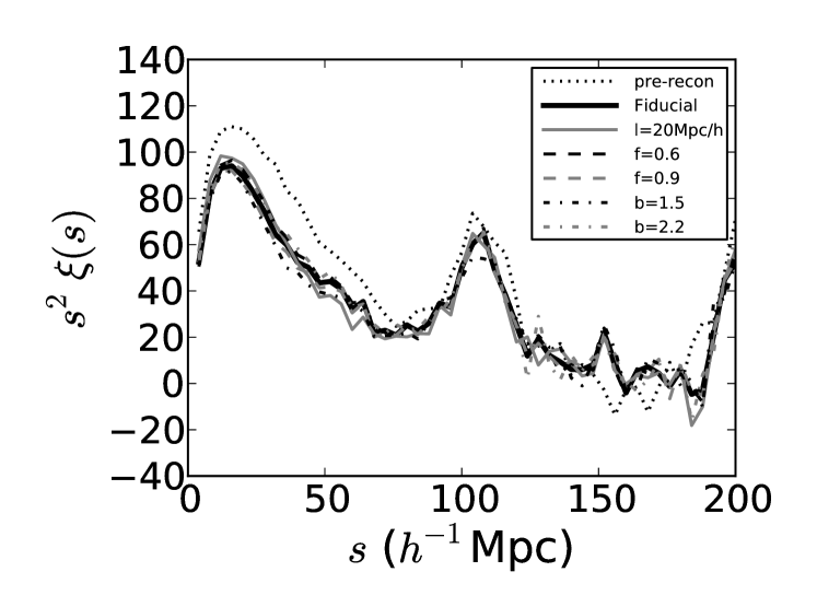
In this section, we test the sensitivity of reconstruction to our fiducial values of the bias , the growth rate , and the smoothing length (used to remove shot noise in the computation of the density field). In order to do this, we run reconstruction in a sample of 100 PTHalos mocks assuming the standard values for all except one of these parameters. In particular, we tested the effect of assuming a bias of and (i.e. 20 per cent below and above the average recovered bias from the mocks, which was adopted as our standard value), and also the effect of assuming a growth rate of and (again, 20 per cent below and above our standard value). We also tested the effect of choosing a more conservative smoothing length of Mpc. As both the correlation function and power spectrum fits give consistent results for our standard reconstruction run (see Section 7), for simplicity in this Appendix we only report results measuring the acoustic scale from the correlation function.
The results are shown at the end of Table 5. On average, different choices for the values of the reconstruction parameters do not bias our distance scale measurements by more than per cent with respect to the measurements using the fiducial values. However, even these small biases are not significant considering their errors. We conclude that our measurements of the distance scale are not sensitive to changes in the fiducial values of the reconstruction parameters over a wide range of values, and in good agreement with the fiducial case.
We also study the dependence on reconstruction parameters of the CMASS DR9 measurements of the distance scale from the correlation function after reconstruction. We select the same cases we studied above for the case of the PTHalos mocks, and run reconstruction on CMASS DR9 galaxies for each choice of the parameters. The results are shown in Table 6. We find that in all cases the distance scale measurements are consistent with the results from the fiducial case. It is worth noting that the choice of a galaxy bias 20 per cent smaller () than the fiducial case drives the measurement and the errors above the rest of the cases. The reason becomes evident in Figure 31, which shows the correlation functions after reconstruction for different values of the reconstruction parameters. The shape of the correlation function around the BAO peak has been distorted by this particular choice of bias, whereas all other choices show results more similar to the fiducial case. This is an indication that our estimates for the galaxy bias and the cosmological parameters cannot be completely arbitrary if we want to reconstruct the density field accurately. However, for reasonable values for these parameters, we do not find a large sensitivity of our measurements to these parameters, and find our results to be consistent with the fiducial case.
B.2 Robustness of Fitting Algorithm for
| Model | rms | Quantiles | rms | Quantiles | |||||
| Before Reconstruction | |||||||||
| Fiducial | 1.004 | 0.027 | 1.004 | – | – | – | – | 39.60/39 | |
| Fit with . | 0.999 | 0.026 | 1.000 | -0.005 | 0.009 | -0.004 | 42.93/42 | ||
| Fit with . | 1.001 | 0.027 | 1.002 | -0.002 | 0.004 | -0.002 | 41.24/40 | ||
| Fit with . | 1.004 | 0.027 | 1.004 | 0.000 | 0.001 | -0.000 | 38.27/38 | ||
| Fit between . | 1.001 | 0.028 | 1.003 | -0.002 | 0.006 | -0.002 | 41.78/41 | ||
| Fit between . | 1.005 | 0.027 | 1.005 | 0.001 | 0.003 | 0.001 | 34.20/34 | ||
| Fit with . | 1.000 | 0.030 | 0.999 | -0.004 | 0.015 | -0.005 | 41.60/39 | ||
| Fit with . | 1.002 | 0.028 | 1.003 | -0.001 | 0.005 | -0.002 | 39.72/39 | ||
| Fit with . | 1.005 | 0.028 | 1.005 | 0.001 | 0.005 | 0.001 | 40.11/39 | ||
| Fit using ML covariance matrix. | 1.003 | 0.029 | 1.005 | -0.001 | 0.008 | -0.000 | 40.07/39 | ||
| After Reconstruction | |||||||||
| Fiducial | 1.004 | 0.018 | 1.004 | – | – | – | – | 40.95/39 | |
| Fit with . | 1.002 | 0.018 | 1.002 | -0.002 | 0.004 | -0.002 | 45.15/42 | ||
| Fit with . | 1.004 | 0.018 | 1.003 | -0.001 | 0.001 | -0.001 | 42.53/40 | ||
| Fit with . | 1.004 | 0.018 | 1.004 | -0.000 | 0.000 | -0.000 | 39.94/38 | ||
| Fit between . | 1.010 | 0.017 | 1.010 | 0.006 | 0.003 | 0.005 | 47.38/41 | ||
| Fit between . | 1.004 | 0.018 | 1.003 | -0.001 | 0.002 | -0.001 | 34.55/34 | ||
| Fit with . | 1.003 | 0.019 | 1.003 | -0.001 | 0.003 | -0.001 | 40.87/39 | ||
| Fit with . | 1.003 | 0.018 | 1.004 | -0.001 | 0.002 | -0.001 | 40.84/39 | ||
| Fit with . | 1.006 | 0.018 | 1.006 | 0.001 | 0.003 | 0.001 | 41.62/39 | ||
| Fit using ML covariance matrix. | 1.004 | 0.019 | 1.003 | -0.000 | 0.004 | -0.000 | 41.02/39 | ||
| Fit to recon. with . | 1.004 | 0.019 | 1.004 | 0.000 | 0.006 | 0.000 | 42.56/39 | ||
| Fit to recon. with . | 1.003 | 0.019 | 1.005 | -0.000 | 0.006 | -0.001 | 41.01/39 | ||
| Fit to recon. with . | 1.003 | 0.018 | 1.004 | -0.000 | 0.002 | -0.000 | 40.50/39 | ||
| Fit to recon. with . | 1.004 | 0.018 | 1.005 | 0.001 | 0.002 | 0.001 | 41.09/39 | ||
| Fit to recon. with . | 1.006 | 0.019 | 1.008 | 0.003 | 0.007 | 0.002 | 45.04/39 | ||
1 , where is the model indicated in the first column.
2 Note that the error on the mean is
smaller than the rms from the mocks quoted in the table, where is
the number of mocks. These much smaller numbers would indicate that
there is a significant detection of the change in the mean as we
change fitting model or reconstruction parameters; however, such a
small change would not be significantly detected in each mock given
the dispersion.
We test the robustness of our correlation function fitting model by slightly varying the fiducial model parameters and then re-performing the fits to see if we recover consistent values of the acoustic scale . These tests are performed on the mocks as well as the CMASS DR9 data. Recall that the fiducial model takes on the form given in Equations (23) and (25), where we have taken before reconstruction and after reconstruction. In addition, we specify a fiducial fitting range of and use the sample covariance matrix. Hence, the fiducial model parameters we alter in performing these tests are the order of , the value of , the fitting range, and the covariance matrix used. In modifying the form of , corresponds to , corresponds to a 2-parameter , and corresponds to a 4-parameter .
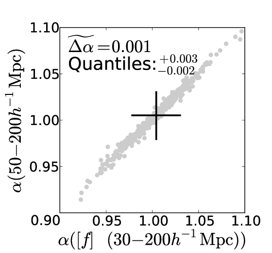
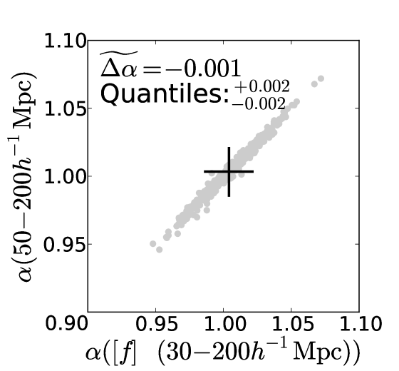
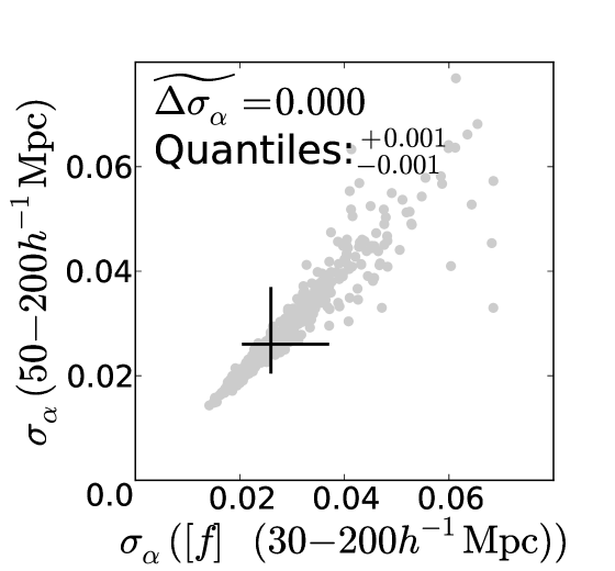
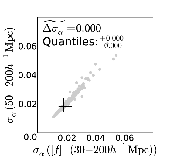
The fiducial and tweaked model fit results for 600 mocks are shown in Table 5. We remove mock results with poorly measured values of since a BAO feature was not clearly identified ( per cent). Nearly perfect 1:1 correlations between the values of are measured from the mocks as shown in Fig. 32. The top two panels of Fig. 32 show the values measured using the fiducial model plotted against the values measured using a smaller fitting range () both before (left) and after (right) reconstruction. The bottom two panels show the corresponding plots for . Similar 1:1 correlations are seen for most of the other “tweaked” models, implying that our fiducial model returns unbiased measurements of the acoustic scale. The only cases that have larger scatter in the correlations are the pre-reconstruction and cases which is not surprising. The prior implies that before reconstruction, there is non-negligible broadband smooth signal that may bias our measurement of the acoustic scale and hence a non-zero form for is required to marginalize over this contribution. The latter implies that using a BAO model that does not account for the effects of non-linear evolution, which are clearly evident before reconstruction, will also bias the measurement of . After reconstruction, the scatter in these cases is greatly reduced as reconstruction partially undoes large-scale redshift space distortions and non-linear structure growth.
Similar results for the CMASS DR9 data are shown in Table 6. In general, our choice of model parameters does not affect the outcome of the fits. A few cases measure slightly larger or smaller values of , but all fall well within the 1 errorbars.
| Model | ||
| Before Reconstruction | ||
| Fiducial | 30.53/39 | |
| Fit with . | 40.84/42 | |
| Fit with . | 30.74/40 | |
| Fit with . | 30.33/38 | |
| Fit between . | 32.47/41 | |
| Fit between . | 22.99/34 | |
| Fit with . | 30.84/39 | |
| Fit with . | 29.93/39 | |
| Fit with . | 32.02/39 | |
| Fit using ML covariance matrix. | 30.64/39 | |
| After Reconstruction | ||
| Fiducial | 34.53/39 | |
| Fit with . | 41.82/42 | |
| Fit with . | 36.12/40 | |
| Fit with . | 33.29/38 | |
| Fit between . | 47.31/41 | |
| Fit between . | 25.94/34 | |
| Fit with . | 34.18/39 | |
| Fit with . | 34.27/39 | |
| Fit with . | 35.10/39 | |
| Fit using ML covariance matrix. | 34.30/39 | |
| Fit to recon. with . | 42.97/39 | |
| Fit to recon. with . | 46.89/39 | |
| Fit to recon. with . | 33.19/39 | |
| Fit to recon. with . | 36.53/39 | |
| Fit to recon. with . | 43.79/39 | |
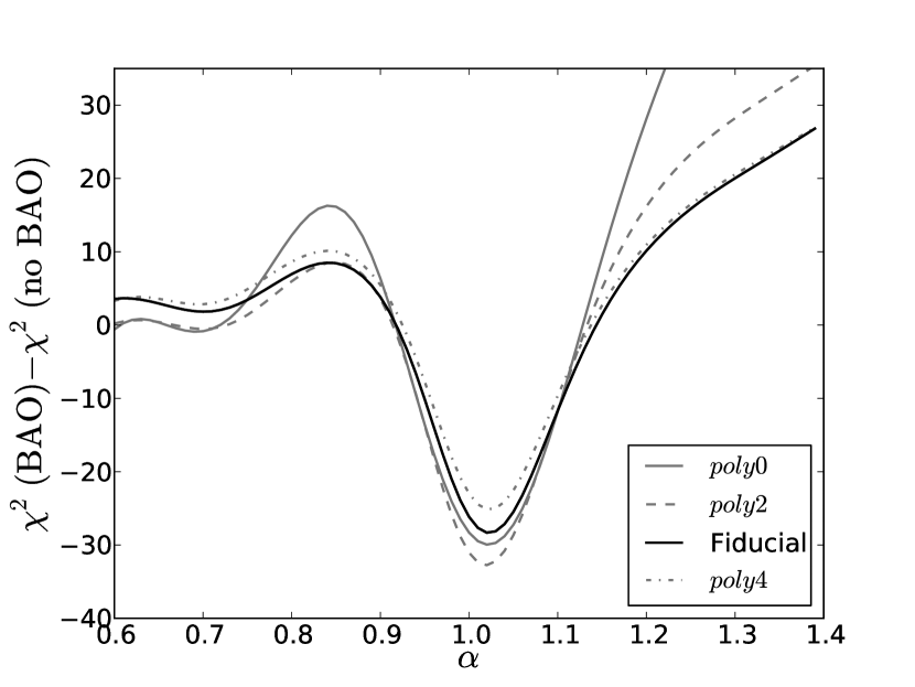
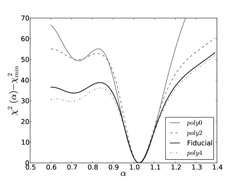
|
We also investigate our measurements of BAO significance with respect to the form of . The results are shown in Fig. 33 after reconstruction. The right panel shows the difference in between a fit to the data using a model containing BAO and a fit to the data using a model without BAO. These curves demonstrate how well we have detected the BAO in the CMASS DR9 data. The solid black curves correspond to subtracting the solid line from the dashed line in Fig. 6. The other lines correspond to various other forms of , some with more and some with less nuisance parameters. Here, the more negative is, the more a model containing BAO is preferred. Allowing more or less flexibility in the broadband marginalization as parameterised by does not change the fact that a model containing BAO is favoured and we have a robust detection of the BAO in the CMASS DR9 data. The actual confidence level changes slightly between the different forms; however, the variation is small and consistently falls between .
The right panel shows the values from the minimum (or best-fit value) and demonstrates how well we have measured the acoustic scale. The solid black curve is identical to the solid line in Fig. 6. The other curves correspond to various other forms of . In all cases, the minima lie at the same value of with the plateaus lying at significant above the minima. Although shows significant variation between the forms, we see at least a () preference for the best-fit value of . It appears that a lower order or less flexible form for may return at a higher confidence, which indicates that higher order may afford the model with enough flexibility to start fitting noise.
We have tested the robustness of the fitting methods by making Gaussian realisations of the correlation function from the full covariance matrix and a template for the correlation function. We have considered the model defined by Eq. 23, and computed the best fit parameters for every simulation. The sample of recovered parameter values that we recovered has a Gaussian distribution, as expected. We also checked that our simulations are truly Gaussian by computing the estimator for each simulation at the “true model” (with , , and ), and verifying that it follows a -distribution with degrees of freedom, which is the number of bins in used in this test. We have found that, while in the NGC the inferred errors from the fits agree very well with the width of the distribution of , in the SGC the measured errors tend to be slightly under-estimated (by about 0.25 ).
B.3 Robustness of Fitting Algorithm for
We have tested that our model for the power spectrum, calculated as described in Section 6.2, provides an adequate match to the power spectra of the mocks. In fact the data plotted in Figs. 8 & 12 already show this result to some extent as we plot the deviation between the measured power spectra and the smooth model: The consistency between the data plotted and the expected BAO model shows that any residual differences between data and model are of significantly lower order than the BAO signal.
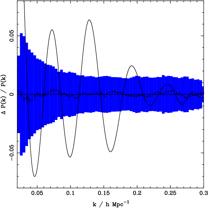
To test the goodness-of-fit further, Fig. 34 displays the average residual recovered after fitting to the 600 power spectra derived from the mock catalogs
| (36) |
where are the measured band powers, and is the best-fit model as defined in Eq. 33. As can be seen in Fig. 34, the average residual is well below the scales of both the BAO and the difference expected for any single fit (shown by the shaded region in Fig. 34), so there is no evidence of a systematic inability to fit the shape of the power spectrum over the fitted -range.

Fig. 35 shows histograms of the recovered best-fit values from the fits to the 600 mock catalogs, before (upper panel) and after (lower panel) reconstruction. These values match the expected distribution of values for a fit with 59 degrees-of-freedom, which is also shown in this plot. This agreement gives us confidence that the fit is behaving as expected for the power spectra derived from the mock catalogues. If the model was unable to adequately fit the mocks, we should expect the recovered minima to be significantly offset from the expected distribution. i.e. if the model failed to adequately fit the shape of the recovered power spectrum, then we would find systematically worse values compared with those expected. The distribution actually agrees remarkably well with that expected, which gives us confidence that the model described in Section 6.2 is adequate for these data.
The values from the fits to the data fall within the distribution of values from the mocks although, for the pre-reconstruction measurement, only 18/600 mocks give a worse value. However, we know from the analysis presented in Section 6.3 that the pre-reconstruction catalogue also gives a smaller-than-average error, so this result is perhaps not that surprising. In conclusion we find no evidence that the fitting method applied to the power spectra is not adequate for recovering the BAO scale.