Abstract

We investigate cosmological consequences of nonlinear sigma model coupled with a cosmological fluid which satisfies the continuity equation. The target space action is of the de Sitter type and is composed of four scalar fields. The potential which is a function of only one of the scalar fields is also introduced. We perform a general analysis of the ensuing cosmological equations and give various critical points and their properties. Then, we show that the model exhibits an exact cosmological solution which yields a transition from matter domination into dark energy epoch and compare it with the $\Lambda$-CDM behavior. Especially, we calculate the age of the Universe and show that it is consistent with the observational value if the equation of the state $\omega_{f}$ of the cosmological fluid is within the range of $0.13<\omega_{f}<0.22.$ Some implication of this result is also discussed.

10.3390/e14091771 14 Received: 21 August 2012; in revised form: 13 September 2012 / Accepted: 17 September 2012 /
Published: 20 September 2012 Exact Solution and Exotic Fluid in Cosmology Seyen Kouwn ¹, Taeyoon Moon ² and Phillial Oh ^1,* E-Mail: ploh@skku.edu; Tel./Fax: 82-031-290-7046/82-031-290-7055

1 Introduction

The recent astronomical measurements revealed that the current Universe is accelerating Riess:1998cb ; Riess:1998cb2 . It is believed that the acceleration is caused by an unknown energy, i.e., dark energy, and grasping the identity of dark energy is one of most fundamental problems in the modern cosmology mukh . Many theoretical models for dark energy have been proposed ever since. Among them, the standard approach is to introduce a cosmological constant wein ; wein2 ; wein3 ; wein4 ; wein5 ; wein6 . In spite of its simplicity and theoretical diversities, it confronts the extreme fine tuning problem. An attractive alternative is to consider that the acceleration is driven by a scalar field. The well known models include quintessence quintessence ; quintessence2 phantom phantom , k-essence k-essence ; k-essence2 ; k-essence3 with the non-canonical kinetic term for the scalar field, and quintom quintom models. In these models various aspects of dark energy can be well described in terms of dynamics of the scalar field and especially, the smallness of the cosmological constant is attributed to the decaying scalar energy density nojiri1 .

On the other hand, dark matter plays a central role in the early Universe in the process of structure formation mukh . Most of the dark matter is the cold dark matter (CDM) which is non-relativistic and non-baryonic. In particular, the CDM model with the cosmological constant $\Lambda$ is established as a standard cosmological model, $\Lambda$-CDM mukh . This model is in good agreements with the CMBR data cmb ; cmb2 ; cmb3 as well as SN Ia data Riess:1998cb ; Riess:1998cb2 . The special feature of $\Lambda$-CDM model is that it assumes the Universe with a zero spatial curvature.

Recently, the dark energy model based on a nonlinear sigma model Lee with or without a cosmological constant was investigated. In this model the target space is noncompact four-dimensional de Sitter manifold and four scalar fields are introduced to account for this. It was found that an exponentially accelerating solution is possible even without the cosmological constant and that the model could describe dark energy interacting with stiff matter even without any matter present. The possibility of other kind of dark matter should be also addressed and it motivates to extend to the more general situation where matter is introduced separately. Therefore, in this paper, we consider more general case of the de Sitter nonlinear sigma model where the matter with the equation of state $\omega_{f}$ and also an exponential potential term for the nonlinear sigma model are added to the action, and we investigate the cosmological consequences.

Recall that in spite of the dynamical explanation of the smallness of the current dark energy density contrary to the cosmological constant, the approaches of  quintessence ; quintessence2 ; phantom ; k-essence ; k-essence2 ; k-essence3 have their own shortcomings. For quintessence model, it has the nice properties of tracking solution and scaling behavior, but it is somewhat difficult to match the equation of state to be close to $-1$, and has its own fine-tuning problem bludman . The phantom model gives favorable result with the equation of state, but it has the issue of quantum instability, even though it is classically stable. The k-essence model has the ghost problem coming from the higher derivative nature of the theory. We do not attempt to address these difficult issues with the introduction of the four scalar fields, but one advantage is the existence of the exact solution, which makes comparisons with $\Lambda$-CDM more direct. ( See Equations (11) and (44).)

Let us mention other salient features of our investigation. The field content consists of a phantom and the triplet fields which are canonical scalar fields. Unlike the ordinary phantom model where Big Rip singularity is known to exist, we have an explicit solution which does not show such a behavior. As far as the exact cosmic solution is concerned, the potential is of a negative exponential form of the scalar field $\phi$. This solution prolongs from the matter-dominated epoch to the dark energy epoch. Recall that in the pure phantom model, the negative kinetic energy prohibits the potential to assume a negative value. In our approach, the triplet of scalar fields provides enough compensating positive energy density such that the weak energy condition is not violated. This exact solution can be exploited to extract some numerical values that can be compared with current observations. In particular, we calculate the age of the Universe and compare with the observations. We find that with a fine-tuning of a couple of parameters, $0.13<\omega_{f}<0.22$ is consistent with the observation. This matter corresponds to an exotic cosmological fluid.

The paper is organized as follows. In Section II, we present a basic analysis of $\Lambda-$CDM model paying attention to the exact cosmological solution and its stability analysis. In Section III, we consider the Einstein gravity coupled with the de Sitter nonlinear sigma model including an exponential potential and cosmological fluid with the equation of state $\omega_{f}$, and discuss the cosmological evolution equations. In Section IV, the stability analysis is performed and various critical points are identified. In Section V, we present the exact cosmological solution for a negative exponential potential and calculate the current age of the Universe. We compare it with the observational data and $\Lambda-$CDM model. Section VI includes conclusion and discussion.

2 $\Lambda$CDM Model

Let us first consider an action in which the Einstein gravity has a cosmological constant (c.c.) term with a matter term:

$$S=\int\,d^{4}x\sqrt{-g}~{}\Big{[}\frac{1}{2\kappa^{2}}(R-\Lambda)+{\cal L}_{matter}\Big{]}$$ (1)

where $\kappa^{2}=8\pi G$. Introducing the standard space-time metric via

$$ds^{2}=-dt^{2}+a^{2}(t)dx_{i}dx^{i}$$ (2)

leads to the following equations:

$$H^{2} = \frac{\kappa^{2}\rho_{m}}{3}+\frac{\Lambda}{3}$$ (3)

$$\dot{H} = -\frac{\kappa^{2}}{2}(1+\omega_{m})\rho_{m}$$ (4)

$$\dot{\rho}_{m} + 3(1+\omega_{m})H\rho_{m}=0$$ (5)

In these expressions, $\omega_{m}$ is the equation of state parameter for the matter term, which satisfies $p_{m}=\omega_{m}\rho_{m}$ when $T^{\mu}_{\nu}=(-\rho_{m},p_{m},p_{m},p_{m})$ are assumed.

In order to check the stability, we introduce the following dimensionless quantities (for $\rho_{m},~{}\Lambda>0$)

$$x=\frac{\kappa\sqrt{\rho_{m}}}{\sqrt{3}H},~{}~{}y=\frac{\sqrt{\Lambda}}{\sqrt{3}H}$$ (6)

From the above quantities, one obtains $x^{\prime}$ and $y^{\prime}$ as ($N\equiv\ln a$)

$$x^{\prime} = \frac{dx}{dN}=\frac{3}{2}(1+\omega_{m})x(x^{2}-1)$$ (7)

$$y^{\prime} = \frac{dy}{dN}=\frac{3}{2}(1+\omega_{m})yx^{2}$$ (8)

The critical points, i.e., the solutions corresponding to $x^{\prime}=0,~{}y^{\prime}=0$ and the eigenvalues for the critical points copeland are given by

$$x_{c} = 0,~{}~{}y_{c}=1~{}(c.c.~{}dominant),~{}~{}~{}~{}~{}~{}~{}\mu_{1}=0,~{}~{}\mu_{2}=-\frac{3}{2}(1+\omega_{m})$$ (9)

$$x_{c} = 1,~{}~{}y_{c}=0~{}(matter~{}dominant),~{}~{}~{}~{}~{}~{}~{}\mu_{1}=3(1+\omega_{m}),~{}~{}\mu_{2}=\frac{3}{2}(1+\omega_{m})$$ (10)

From these eigenvalues we see that the matter dominant phase is unstable for $\omega_{m}>-1$ while c.c. dominant phase has a decaying mode, i.e., $\mu_{2}<0$ being stable. (The existence of a zero eigenvalue ($\mu_{1}=0$) in Equation (9) is originated from the fact that two variables $x$ and $y$ are connected by the relation $x^{2}+y^{2}=1$. Therefore in this case one can reduce to one$-$dimensional space Alimohammadi .) It is well-known that there exists the non-perturbative solution of Equations (3)–(5) which connects these two critical points as

$$a(t)=a_{*}(\sinh[At])^{2/3(1+\omega_{m})},~{}~{}~{}H(t)=\sqrt{\frac{\Lambda}{3}}\coth[At],~{}~{}~{}\rho_{m}=\frac{\Lambda}{\kappa^{2}}(\sinh[At])^{-2}$$ (11)

where $A=(1+\omega_{m})\sqrt{3\Lambda}/2$. This solution describes a smooth transition from matter-dominated power law expansion at early times into cosmological constant-dominated exponential acceleration at late times.

To check the stability of the above solutions Equation (11), we consider the variation of Equations (3)–(5), which yields

$$2H\delta{H} = \frac{\kappa^{2}}{3}\delta\rho_{m}$$ (12)

$$\delta\dot{H} = -\frac{\kappa^{2}}{2}(1+\omega_{m})\delta{\rho}_{m}$$ (13)

$$\delta\dot{\rho}_{m} + 3(1+\omega_{m})\rho_{m}\delta H+3(1+\omega_{m})H\delta\rho_{m}=0$$ (14)

Then we find the solution for the above Equations (12)– (14) as

$$\delta H=BC\tanh[At]e^{-f(t)}/\kappa^{2},~{}~{}~{}\delta\rho_{m}=Ce^{-f(t)}/\kappa^{4}$$ (15)

where $B=(1+\omega_{m})/4A$, $C$ is an arbitrary constant and $f(t)=-2At+\ln[-1+e^{4At}]+2\ln[\tanh[At]]$.
Note that $f(t)$ approaches $2At$ as $t\rightarrow\infty$ and both $\delta H$ and $\delta\rho_{m}$ decay, which implies that the solution (11) is stable.

Introducing the dimensionless density parameters $\Omega_{m}=\kappa^{2}\rho_{m}/3H^{2}$ and $\Omega_{\Lambda}=\Lambda/3H^{2}$, Equation (3) becomes

$$\Omega_{m}+\Omega_{\Lambda}=1$$ (16)

Particularly for the solution (11), $\Omega_{m}$ and $\Omega_{\Lambda}$ are given by

$$\Omega_{m}=\frac{1}{(\cosh[At])^{2}},~{}~{}~{}\Omega_{\Lambda}=1-\frac{1}{(\cosh[At])^{2}}$$ (17)

By using the experimental data, i.e., $\rho_{\Lambda}=\frac{\Lambda c^{2}}{8\pi G}\sim(10^{-12}Gev)^{4}\sim 10^{-8}erg/cm^{3}$, $H_{0}\sim 2.28\times 10^{-18}s^{-1}$ and the solution $H_{0}=\sqrt{3\Lambda}\coth[At_{0}]/3$, we can evaluate the value $At_{0}=1.27$. From these values we find $\Omega_{\Lambda}$ and $t_{0}$ for the dust-like matter ($\omega_{m}=0$) as

$$\Omega_{\Lambda}\approx 0.73,~{}~{}~{}t_{0}\approx 4.34\times 10^{17}s$$ (18)

which are in agreement with the observational data komatsu .

3 de Sitter Nonlinear Sigma Model with Potential

In this section, we extend the analysis performed in the case of $\Lambda-$CDM to the de Sitter nonlinear sigma model Lee with a potential term. The cosmological fluid with the equation of state $\omega_{f}$ is also added. The starting action is

$$S=\int\,d^{4}x\sqrt{-g}~{}[~{}\frac{1}{2\kappa^{2}}R-\frac{g^{\mu\nu}}{\lambda^{2}}G_{\alpha\beta}(\Phi)\partial_{\mu}\Phi^{\alpha}\partial_{\nu}\Phi^{\beta}-\epsilon V(\phi)+{\cal L}_{fluid}~{}]$$ (19)

where $\Phi^{\alpha}=(\phi,\sigma^{i})~{}(i=1,2,3)$, $\lambda$ is a dimensionless coupling constant and $\epsilon=\pm 1$. Here $G_{\alpha\beta}$ is the metric of the de Sitter target space,

$$G_{\alpha\beta}=(-1,~{}+e^{2\kappa\xi\phi},~{}+e^{2\kappa\xi\phi},~{}+e^{2\kappa\xi\phi}~{})$$ (20)

where $\xi$ is an arbitrary positive constant and $V(\phi)$ is the potential given by

$$V(\phi)=V_{0}\exp(-\kappa\gamma\phi)$$ (21)

with an arbitrary constant $\gamma$ and $V_{0}>0$. Among diverse possibilities, we have chosen exponential potential. A couple of reasons could be cited. The first one is that this potential is the prototype which gives rise to accelerating Universe and has interesting properties like scaling solution and attractor in the quintessence cope or phantom model copeland . The second one is that it can yield non-perturbative solution of the type discussed in the previous section in our case for the negative potential with $\epsilon=-1$. We regard the second and third terms of Equation (19) as representing the dark energy sector. For the matter part, we assume a cosmological fluid of the perfect fluid form, $T^{\mu}_{\nu}=(-\rho_{f},~{}p_{f},~{}p_{f},~{}p_{f})$, which satisfies the continuity equation, $\nabla_{\mu}T^{\mu\nu}=0.$

We first note that the following ansatz

$$\sigma^{i}=x^{i}$$ (22)

solves the $\sigma^{i}$ field equations. The above ansatz first appeared in higher dimensional gravity theory in association with spontaneous compactification of the extra dimensions omero ; gellmann ; gellmann2 ; gellmann3 . It was revived in four dimensions recently in describing the accelerating Universe with the de Sitter nonlinear sigma model Lee . Note that it does not break the isotropy and homogeneity of the universe as long as we do not introduce the potential for the $\sigma$ fields. With this ansatz, the standard space-time metric Equation (2), and $\phi=\phi(t)$, the evolution equations, are given by

$$H^{2} = \frac{2\kappa^{2}}{3\lambda^{2}}~{}\Big{[}~{}-\frac{1}{2}\dot{\phi}^{2}+\frac{3}{2\kappa^{4}a^{2}}e^{2\kappa\xi\phi}+\frac{\epsilon\lambda^{2}}{2}V(\phi)~{}\Big{]}+\frac{\kappa^{2}}{3}\rho_{f}$$ (23)

$$\dot{H} = -\frac{\kappa^{2}}{\lambda^{2}}\Big{[}~{}-\dot{\phi}^{2}+\frac{1}{\kappa^{4}a^{2}}e^{2\kappa\xi\phi}~{}\Big{]}-\frac{\kappa^{2}}{2}(1+\omega_{f})\rho_{f}$$ (24)

$$0 = \ddot{\phi}+3H\dot{\phi}-3\xi\frac{e^{2\kappa\xi\phi}}{\kappa^{3}a^{2}}+\frac{\epsilon\kappa\gamma\lambda^{2}}{2}V_{0}e^{-\kappa\gamma\phi}$$ (25)

and the continuity equation implies $\rho_{f}=\rho(0)[a(t)/a(0)]^{-3(1+\omega_{f})},$ where $\omega_{f}$ is a barotropic equation of state with $0<\omega_{f}<1$. We mention a couple of properties of the above evolution equations. The first one is that in spite of the $\phi$ being a phantom, the presence of the second term in Equation (24) that comes from the spatial variations of $\sigma^{i}$ fields could prevent the Big Rip singularity from being developed; it is not guaranteed that $\dot{H}$ will stay always positive at late times when $\rho_{f}$ is ignored. The other is that even in the $\epsilon=-1$ case, the weak energy condition could not be violated (in the ordinary phantom model with a negative potential, the weak energy condition is always violated because of $\rho_{\phi}=-\dot{\phi}^{2}/2-V(\phi)<0$). This again is due to the the second terms in Equations (23) and (24) coming from the spatial variations. In fact, we will show that for $\epsilon=-1$ there exists an exact cosmological solution of the type discussed in $\Lambda-$CDM case, which interpolates between matter-dominated and dark energy-dominated epochs.

4 Stability

To perform the stability analysis and figure out the energy dominance of the kinetic ($x$), spatial ($y$) and potential ($z$) parts in Equation (23), we first introduce the following dimensionless quantities,

$$x\equiv\frac{\kappa\dot{\phi}}{\sqrt{3}\lambda H},~{}~{}y\equiv\frac{e^{\kappa\xi\phi}}{\kappa\lambda Ha},~{}~{}z\equiv\frac{\kappa\sqrt{V}}{\sqrt{3}H}$$ (26)

Then the constraint Equation (23) is given by

$$-x^{2}+y^{2}+\epsilon z^{2}+\frac{\kappa^{2}\rho_{f}}{3H^{2}}=1$$ (27)

With $N=\ln{a}$, we obtain

$$x^{\prime} \equiv \frac{dx}{dN}\!=\!\frac{x}{2}[-3(1\!-\!\omega_{f})x^{2}-(1+3\omega_{f})y^{2}\!+\!3(-1\!+\!\omega_{f})-3\epsilon(1\!+\!\omega_{f})z^{2}]-\frac{3\epsilon\bar{\gamma}}{\sqrt{6}}z^{2}\!+\!\bar{\xi}\sqrt{6}y^{2}$$ (28)

$$y^{\prime} \equiv \frac{dy}{dN}=\frac{y}{2}[-3(1-\omega_{f})x^{2}-(1+3\omega_{f})y^{2}\!+(1+3\omega_{f})-3\epsilon(1+\omega_{f})z^{2}+2\bar{\xi}\sqrt{6}x]$$ (29)

$$z^{\prime} \equiv \frac{dy}{dN}=\frac{z}{2}[-3(1-\omega_{f})x^{2}-(1+3\omega_{f})y^{2}+3(1+\omega_{f})-3\epsilon(1+\omega_{f})z^{2}-\sqrt{6}\bar{\gamma}x]$$ (30)

where $\bar{\gamma}=\lambda\gamma/\sqrt{2},~{}\bar{\xi}=\lambda\xi/\sqrt{2}$. The various critical points and their properties including the stabilities of the above equations are summarized in Table 1 with their eigenvalues being given as follows:

• point A

  $$\mu_{1}=\frac{3}{2}(\omega_{f}-1),~{}~{}\mu_{2}=\frac{1+3\omega_{f}}{2},~{}~{}\mu_{3}=\frac{3(\omega_{f}+1)}{2}$$ (31)

• point B

  $$\mu_{1,2}=-\frac{3(1-\omega_{f})}{4}\pm\frac{\sqrt{\bar{\gamma}^{2}(-1+\omega_{f})(24+24{\omega_{f}}^{2}+7\bar{\gamma}^{2}+\omega_{f}(48+9\bar{\gamma}^{2}))}}{4\bar{\gamma}^{2}}$$ (32)

  $$\mu_{3}=\frac{\bar{\gamma}+3\omega_{f}\bar{\gamma}+6(1+\omega_{f})\bar{\xi}}{2\bar{\gamma}}$$ (33)

• point C

  $$\mu_{1,2}=-\frac{3(1-\omega_{f})}{4}\pm\frac{\sqrt{\bar{\xi}^{2}(-1+\omega_{f})(4(1+3\omega_{f})^{2}+3(5+27\omega_{f})\bar{\xi}^{2})}}{4\bar{\xi}^{2}}$$ (34)

  $$\mu_{3}=\frac{\bar{\gamma}+3\omega_{f}\bar{\gamma}+6(1+\omega_{f})\bar{\xi}}{4\bar{\xi}}$$ (35)

• point D

  $$\mu_{1}=-\frac{6+\bar{\gamma}^{2}}{2},~{}~{}\mu_{2}=-3-3\omega_{f}-\bar{\gamma}^{2},~{}~{}\mu_{3}=-\frac{2+\bar{\gamma}^{2}+2\bar{\gamma}\bar{\xi}}{2}$$ (36)

• point E

  $$\mu_{1}=-1-3\omega_{f}-6\bar{\xi}^{2},~{}~{}\mu_{2}=1-3\bar{\xi}^{2}-\frac{3\bar{\gamma}\bar{\xi}}{2},~{}~{}\mu_{3}=-2-3\bar{\xi}^{2}$$ (37)

• point F

  $$\mu_{1,2}=-\frac{\bar{\gamma}+3\bar{\xi}}{\bar{\gamma}+2\bar{\xi}}\pm\frac{\sqrt{-(8-6\bar{\gamma}\bar{\xi}(\bar{\gamma}+2\bar{\xi})^{2})-3\bar{\gamma}^{2}+10\bar{\gamma}\bar{\xi}+33\bar{\xi}^{2}}}{\bar{\gamma}+2\bar{\xi}}$$ (38)

  $$\mu_{3}=-\frac{\bar{\gamma}+3\omega_{f}\bar{\gamma}+6(1+\omega_{f})\bar{\xi}}{\bar{\gamma}+2\bar{\xi}}$$ (39)

Note that all of the above eigenvalues of the critical points do not have any $\epsilon$-dependence even though the various critical points themselves carry its dependence.

Table 1: The classification and the properties of the critical points.

In Table 1, the second to fourth columns denote energy contents of the dark energy sector, the fifth column shows the conditions for the existence of the solutions of the critical Equations (28)–(30). The critical points B and F are further divided for $\epsilon=\pm 1$. The sixth column is about the stability condition for each eigenvalue. In the seventh column, $\Omega_{\phi}=-x^{2}+y^{2}+\epsilon z^{2}$ is the density parameter for the dark energy, and the last column displays the equation of state for the dark energy. First, we note that the results of phases A, B2, D with $\epsilon=+1$ and $y=0$ agree with those in the literature copeland , which correspond to the phantom with a positive potential. In particular, the system approaches the scalar-dominated solution D with non-relativistic dark matter $(\omega_{f}=0)$. The point F2 also corresponds to scalar-dominated solution but with a non-zero value of $y$.

Let us focus on the $\epsilon=-1$ case from here on. Then, points E and F1 both give scalar-dominated solutions. Which solution will the system choose depends on the allowed parameters for the existence and stability conditions and on the initial conditions. For solution E, $z=0$ and $\omega_{\phi}$ approaches to $-1$ when $\bar{\xi}^{2}\rightarrow 1/3$. On the other hand, for solution F, all $x$, $y$ and $z$ contribute to the dark energy and $\omega_{\phi}$ converges to $-1$ when $\bar{\xi}$ goes to infinity. In the next section, we present an explicit solution of Equations (23)–(25), which prolongs from B1 at early times to E at late times.

5 Exact Cosmological Solution

In order to investigate the exact solution for Equations (23)–(25), we first assume that $a=e^{\kappa\xi\phi}/\sqrt{f}$, which corresponds to $H=\kappa\xi\dot{\phi}$. Here $f$ is an arbitrary constant at this stage. In the case of $\epsilon=-1$, from the above ansatz one can find an exact solution as follows:

$$\phi(t) = \phi(0)+\frac{\sqrt{f}}{\kappa^{2}}t+\frac{2}{3\kappa\xi(1+\omega_{f})}\ln\left[\frac{1+Ce^{-3\xi(1+\omega_{f})t/\kappa}}{1+C}\right]$$ (40)

where $C$ is an arbitrary constant and $V_{0}$ and $\rho_{0}$ are given by

$$V_{0} = \frac{f(1-\omega_{f})}{\kappa^{4}\lambda^{2}(1+\omega_{f})}e^{3(1+\omega_{f})\kappa\xi\phi(0)}\left\{\frac{(1+C)^{2}}{-4C}\right\}$$ (41)

$$\rho_{0} = \frac{-4Cf}{\kappa^{4}(1+C)^{2}}\left\{3\xi^{2}+2\frac{1}{(1+\omega_{f})\lambda^{2}}\right\}$$ (42)

with $\xi^{2}=2/3\lambda^{2}$, $\gamma=3(1+\omega_{f})\xi$. It is to be noticed that $C$ should be a negative value to preserve the weak energy condition. In this case, introducing a time scale defined by $|C|=e^{-3\frac{\xi}{\kappa}(1+\omega_{f})\sqrt{f}t_{*}}$, Equation (40) and $a=e^{\kappa\xi\phi}/\sqrt{f}$ reduce to

$$\phi(t) = \frac{2}{3\kappa\xi(1+\omega_{f})}\ln\left(\sinh\left[\frac{3(1+\omega_{f})}{2}\frac{\xi}{\kappa}\sqrt{f}(t+t_{*})\right]\right)+\tilde{\phi}(0)$$ (43)

$$a(t) = \tilde{a}\sinh\left[\frac{3(1+\omega_{f})}{2}\frac{\xi}{\kappa}\sqrt{f}(t+t_{*})\right]^{\frac{2}{3(1+\omega_{f})}}$$ (44)

where $\tilde{\phi}(0)=\phi(0)-2\ln\Big{[}\sinh(\frac{3(1+\omega_{f})}{2}\frac{\xi}{\kappa}\sqrt{f}t_{*})\Big{]}/(3(1+\omega_{f})\kappa\xi)$ and $\tilde{a}=e^{\kappa\xi\tilde{\phi}(0)}/\sqrt{f}$

We note that for $t\to-t^{*}$ the solution (44) behaves as $a\sim t^{2/(3(1+\omega_{f}))}$, which shows that it represents an expanding Universe with cosmological fluid $\omega_{f}$, whereas at late times, it represents an accelerating Universe with $a(t)\sim e^{\xi\sqrt{f}t/{\kappa}}$. Now, let us check that the above solution indeed corresponds to the one that prolongs from B1 at early times to E at late times, as was mentioned in the previous section. To this end we first substitute the solutions (41)–(44) into the dimensionless quantities $x,~{}y,~{}z$ of Equation (26). Then one can find

$$x = \frac{1}{\sqrt{3}\lambda\xi}$$ (45)

$$y = \frac{1}{\lambda\xi}\frac{\sinh[\frac{3(1+\omega_{f})}{2}\frac{\xi}{\kappa}\sqrt{f}(t+t_{*})]}{\cosh[\frac{3(1+\omega_{f})}{2}\frac{\xi}{\kappa}\sqrt{f}(t+t_{*})]}$$ (46)

$$z = \frac{1}{\sqrt{3}\lambda\xi}\frac{(\frac{1-\omega_{f}}{1+\omega_{f}})^{\frac{1}{2}}}{\cosh[\frac{3(1+\omega_{f})}{2}\frac{\xi}{\kappa}\sqrt{f}(t+t_{*})]}$$ (47)

When choosing $\xi=\sqrt{2}/\sqrt{3}\lambda(\bar{\xi}=1/\sqrt{3})$, we see that at early times, i.e., $t\to-t^{*}$, the quantities $x,~{}y,~{}z$ of Equations (45)–(47) are given by

$$x=\frac{1}{\sqrt{2}},~{}~{}y=0,~{}~{}z=\sqrt{\frac{1-\omega_{f}}{2(1+\omega_{f})}}$$

and at late times ($t\to\infty$) they become

$$x=\frac{1}{\sqrt{2}},~{}~{}y=\sqrt{\frac{3}{2}},~{}~{}z=0$$

If we identify $\bar{\gamma}=(1+\omega_{f})\sqrt{3}$, and substituting $\bar{\xi}=1/\sqrt{3}$ into B1 and E of Table 1, we exactly find the above values of $x$, $y$ and $z$. Therefore, we conclude that our solution corresponds to the phase B1 at early times and to the phase E at late times.

We now determine the allowed range of $\omega_{f}$ for this exact solution by comparing with the current observational data. It turns out that the non-relativistic dark matter with $\omega_{f}=0$ is not consistent with the current value of $t_{0}$. To carry out this in detail, we recall the density parameter of the scalar field given by (we set $t_{*}\sim 0$)

$$\Omega_{\phi} = -x^{2}+y^{2}-z^{2}$$ (48)

$$= (\tanh[Bt])^{2}-\frac{1}{(1+\omega_{f})(\cosh[Bt])^{2}}$$

where $B=3(1+\omega_{f})\xi\sqrt{f}/2\kappa$ with $\xi=\sqrt{2}/\sqrt{3}\lambda$ and the Hubble parameter

$$H = \frac{2B}{3(1+\omega_{f})}\coth[Bt]$$ (49)

We first comment on the dependence of $\Omega_{\phi}$, and $H$ of Equations (48) and (49) on the initial conditions. The exact solutions, Equations (43) and (44), show the dependence of $\phi$ and $a$ on the initial conditions. However, the dependence of the quantities $x,~{}y,~{}$ and $z$ on the initial conditions are absent as can be seen in the expressions of Equations  (45)–(47). This may be due to the fact that our exact cosmological solution satisfies the condition $a=e^{e^{\kappa\xi\phi}}/\sqrt{f}$ and is of a non-perturbative nature. The only remaining dependence is through the variable $t_{*}$, which we have set to zero without loss of generality. Therefore, $\Omega_{\phi}$ and $H$ of Equations (48) and (49) are insensitive to the initial conditions as far as the non-perturbative solutions (43) and (44) are concerned. This aspect is rather unexpected because there is a priori no reason why the quantities $x$, $y$ and $z$ defined in Equation (26) should not depend on the initial conditions of $\phi$ and $a$.

In the above two Equations (48) and (49), we treat $\Omega_{\phi,0}$, $H_{0}$ at $t=t_{0}$ as input parameters to determine $\xi\sqrt{f}$ and especially $\omega_{f}$. Since the observational data komatsu $\Omega_{\phi,0}\simeq 0.726\pm 0.015,~{}H_{0}\simeq 2.28\pm 0.04\times 10^{-18}s^{-1}$ and $t_{0}\simeq 4.33\pm 0.04\times 10^{17}s$ are given with experimental uncertainty, these equations give permitted range of $\omega_{f}$. We use the strategy that we first pick up a specific value of $\omega_{f}$. Then, Equations (48) and (49) will give allowed ranges of $B$ for $\Omega_{\phi,0}$ and $H_{0}$ respectively. We can plot these quantities in ($B,t$)-plane. If there exist intersecting region, then, this value of $\omega_{f}$ is allowed. The results are displayed in Figure 1. We find that for values of $\omega_{f}<0.13$ and $\omega_{f}>0.22$, there does not exist a region intersected by the bands of $\Omega_{\phi,0},~{}H_{0}$ and $t_{0}$. Therefore, we conclude that the allowed value $\omega_{f}$ consistent with the current observational data is given by $0.13<\omega_{f}<0.22$, which corresponds to an exotic cosmological fluid with non-vanishing pressure.

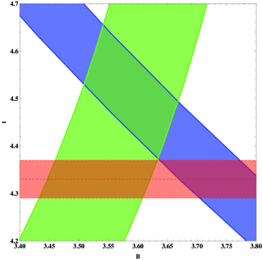
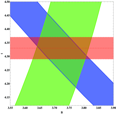
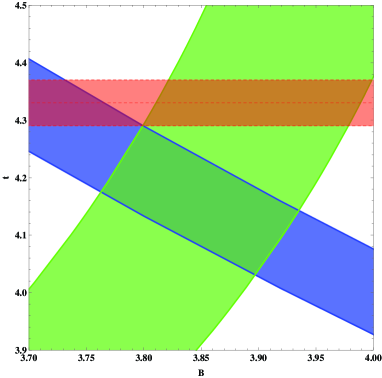
Figure 1: The plot of $\Omega_{\Lambda,0}(blue)\simeq 0.726\pm 0.015,~{}H_{0}(green)\simeq 2.28\pm 0.04\times 10^{-18}s^{-1}$ on the ($B$, $t$)-plane for $\omega_{f}=0.13$(left),  $\omega_{f}=0.18$(right),  $\omega_{f}=0.22$(lower). The red band is the current age with uncertainty $t_{0}\simeq 4.33\pm 0.04\times 10^{17}s$.

6 Conclusion

In this paper, we have investigated various cosmological consequences of the de Sitter nonlinear sigma model with the exponential potential and cosmological fluid term. It consists of a phantom and triplet scalar fields. We have displayed that the presence of the triplet $\sigma$ fields with isotropic spatial dependence provides contrasting features to the phantom model without such fields. For example, the energy and pressure coming from the spatial variations could prevent the Big Rip singularity from being developed. In particular, we found an exact cosmological solution in the case of a negative potential. In this solution, the Universe undergoes a power law expansion at early times as in $\Lambda-$CDM. But the difference is that unlike the $\Lambda-$CDM we have a non-vanishing scalar energy contribution ($x\neq 0,z\neq 0$ of B1 phase) even in the matter dominated epoch. At late times, a complete dark energy-dominance is achieved with $\Omega_{\phi}=1$ and $\omega_{\phi}=-1$ with a suitable choice of the parameter.

The Hubble parameter Equation (49) is exactly the same as $H$ of $\Lambda-$CDM in Equation (11) when we identify the parameter as $\xi\sqrt{3f}/\kappa=\sqrt{\Lambda}$. However, with this choice, one can check that the energy density $\rho_{f}$ of cosmological fluid is different from the matter density $\rho_{m}$ of Equation (11) in $\Lambda-$CDM, and is given by $\rho_{f}/\rho_{m}=1+1/(\omega_{f}+1)$. Note that for $0\leq\omega_{f}\leq 1$, $\rho_{f}$ is always greater than $\rho_{m}$. Also, the dark energy density from Equation (48) approaches $\Lambda/\kappa^{2}$ asymptotically from below. These show that even if the scale factors in both cases behave exactly the same, there exist qualitative differences between the two approaches.

We also have shown that to be consistent with the observational data, the equation of state for the cosmological fluid has to be within the range $0.13<\omega_{f}<0.22$ unlike $\Lambda-$CDM with a dust like matter. This range of $\omega_{f}$ appears in the literature exotic ; exotic2 corresponding to cosmic strings with $-1/3<\omega_{f}<1/3$ or domain walls with $-2/3<\omega_{f}<1/3$. We notice that in $\Lambda-$CDM model, the dark matter has the perfect fluid form and admits a barotropic equation of state. In this case, the dark matter should be pressureless in order to be in accordance with the observational data. However, it is known Bharadwaj ; Su that the dark matter can also be described by an anisotropic fluid but only in the case of non-zero effective pressure or a polytropic equation of state Boehmer . On the other hand, our exotic cosmological fluid not only satisfies a barotropic equation of state but also takes a perfect fluid form. In spite of this, it should have non-zero pressure to be in agreement with the observational data.

We conclude with the following remark. We found that with $\omega_{f}=0$ the evolution is exactly that of $\Lambda$-CDM. But this does not fit the observational data as was discussed, e.g., $\omega_{f}$ has to be in the range of 0.13 and 0.22 to give the observed age of the universe. We speculate that this feature of deviation from the $\Lambda$-CDM for general time-varying dark energy density holds in general. That is, in models where dark energy density varies, the dark matter with $\omega_{m}=0$ might have some difficulty in fitting the observations. Nevertheless, this does not imply that the dynamical dark energy models with non-zero equation of state dark matter must be excluded, and it remains to be seen whether the exotic cosmological fluid considered in this work could be related to the realistic dark matter candidates.

References

- (1) Perlmutter, S.; Aldering, G.; Goldhaber, G.; Knop, R.A.; Nugent, P.; Castro, P.G.; Deustua, S.; Fabbro, S.; Goobar, A.; Groom, D.E.; et al. Measurements of Omega and Lambda from 42 high redshift supernovae. Astrophys. J. 1999, 517, 565–586.
- (2) Riess, A.G.; Filippenko, A.V.; Challis, P.; Clocchiatti, A.; Diercks, A.; Garnavich, P.M.; Gilliland, R.L.; Hogan, C.J.; Jha, S.; Kirshner, R.P.; et al. Observational evidence from supernovae for an accelerating universe and a cosmological constant. Astron. J. 1998, 116, 1009–1038.
- (3) Mukhanov, V. Physical Foundations of Cosmology; Cambridge University Press: Cambridge, UK, 2005.
- (4) Weinberg, S. The cosmological constant problem. Rev. Mod. Phys. 1989, 61, 1–23.
- (5) Carroll, S.M.; Press, W.H.; Turner, E.L. The cosmological constant. Ann. Rev. Astron. Astrophys. 1992, 30, 499–542.
- (6) Sahni, V.; Starobinsky, A.A. The case for a positive cosmological Lambda term. Int. J. Mod. Phys. 2000, D9, 373–444.
- (7) Padmanabhan, T. Cosmological constant: The weight of the vacuum. Phys. Rept. 2003, 380, 235–320.
- (8) Padmanabhan, T. Dark energy: The cosmological challenge of the millennium. Curr. Sci. 2005, 88, 1057.
- (9) Peebles, P.J.E.; Ratra, B. The cosmological constant and dark energy. Rev. Mod. Phys. 2003, 75, 559–606.
- (10) Wetterich, C. Cosmology and the fate of dilatation symmetry. Nucl. Phys. 1988, B302, 668.
- (11) Zlatev, I.; Wang, L.-M.; Steinhardt, P.J. Quintessence, cosmic coincidence, and the cosmological constant. Phys. Rev. Lett. 1999, 82, 896–899.
- (12) Caldwell, R.R. A phantom menace?. Phys. Lett. 2002, B545, 23–29.
- (13) Chiba, T.; Okabe, T.; Yamaguchi, M. Kinetically driven quintessence. Phys. Rev. 2000, D62, doi:10.1103/PhysRevD.62.023511.
- (14) Armendariz-Picon, C.; Mukhanov, V.F.; Steinhardt, P.J. A dynamical solution to the problem of a small cosmological constant and late time cosmic acceleration. Phys. Rev. Lett. 2000, 85, 4438–4441.
- (15) Armendariz-Picon, C.; Mukhanov, V.F.; Steinhardt, P.J. Essentials of k essence. Phys. Rev. 2001, D63, doi:10.1103/PhysRevD.63.103510.
- (16) Feng, B.; Wang, X.-L.; Zhang, X.-M. Dark energy constraints from the cosmic age and supernova. Phys. Lett. 2005, B607, 35–41.
- (17) Bamba, K; Capozziello, S; Nojiri, S.; Odintsov, S.D. Dark energy cosmology: The equivalent description via different theoretical models and cosmography tests. Astrophys Space Sci. 2012, doi: 10.1007/s10509-012-1181-8.
- (18) Bennett, C.L.; Halpern, M.; Hinshaw, G.; Jarosik, N.; Kogut, A.; Limon, M.; Meyer, S.S.; Page, L.; Spergel, D.N.; Tucker, G.S.; et al. First year Wilkinson Microwave Anisotropy Probe (WMAP) observations: Preliminary maps and basic results. Astrophys. J. Suppl. 2003, 148, doi:10.1086/377253.
- (19) Spergel, D.N.; Verde, L.; Peiris, H.V.; Komatsu, E.; Nolta, M.R.; Bennett, C.L.; Halpern, M.; Hinshaw, G.; Jarosik, N.; Kogut, A.; et al. First year Wilkinson Microwave Anisotropy Probe (WMAP) observations: Determination of cosmological parameters. Astrophys. J. Suppl. 2003, 148, 175–194.
- (20) Spergel, D.N.; Bean, R.; Dore, O.; Nolta, M.R.; Bennett, C.L.; Dunkley, J.; Hinshaw, G.; Jarosik, N.; Komatsu, E.; Page, L.; et al. Wilkinson Microwave Anisotropy Probe (WMAP) three year results: Implications for cosmology. Astrophys. J. Suppl. 2007, 170, doi:10.1086/513700.
- (21) Lee, J.; Lee, T.H.; Moon, T.Y.; Oh, P. De-Sitter nonlinear sigma model and accelerating universe. Phys. Rev. 2009, D80, doi:10.1103/PhysRevD.80.065016 .
- (22) Bludman, S. Tracking quintessence would require two cosmic coincidences. Phys. Rev. 2004, D69, 122002:1–122002:8 .
- (23) Copeland, E.J.; Sami, M.; Tsujikawa, S. Dynamics of dark energy. Int. J. Mod. Phys. 2006, D15, 1753–1936.
- (24) Alimohammadi, M.; Ghalee, A. The phase-space of generalized Gauss-Bonnet dark energy. Phys. Rev. 2009, D80, 043006.
- (25) Komatsu, E.; Dunkley, J.; Nolta, M.R.; Bennett, C.L.; Gold, B.; Hinshaw, G.; Jarosik, N.; Larson, D.; Limon, M.; Page, L.; et al. Five-Year Wilkinson Microwave Anisotropy Probe (WMAP) Observations: Cosmological Interpretation. Astrophys. J. Suppl. 2009, 180, 330–376.
- (26) Copeland, E.J.; Liddle, A.R; Wands, D. Exponential potentials and cosmological scaling solutions. Phys. Rev. 1998, D57, 4686–4690.
- (27) Omero, C.; Percacci, R. Generalized nonlinear sigma models in curved pace and space compactification. Nucl. Phys. 1980, B165, 351–364.
- (28) Gell-Mann, M.; Zwiebach, B. Dimensional reduction of space-time induced by nonlinear scalar dynamics and noncompact extra dimensions. Nucl. Phys. 1985, B260, 569-592.
- (29) Gell-Mann, M.; Zwiebach, B. Curling up two spatial dimensions with . Phys. Lett. 1984, B147, 111-114.
- (30) Gell-Mann, M.; Zwiebach, B. Space-time compactification due to scalars. Phys. Lett. 1984, B141, 333-336.
- (31) Kolb, E.W.; Turner, M.S. The Early Universe; Addison-Wesley, Reading, MA, USA, 1990.
- (32) Jafarizadeh, M.A.; Darabi, F.; Rezaei-Aghdam, A.; Rastegar, A.R. Tunneling in Lambda decaying cosmologies and the cosmological constant problem. Phys. Rev. 1999, D60, doi:10.1103/PhysRevD.60.063514.
- (33) Bharadwaj, S.; Kar, S. Modeling galaxy halos using dark matter with pressure. Phys. Rev. 2003, D68, 023516:1–023516:5.
- (34) Su, K.-Y.; Chen, P. Comments on ‘Modeling Galaxy Halos Using Dark Matter with Pressure’. Phys. Rev. 2009, D79, 128301:1–128301:3.
- (35) Boehmer, C.G.; Harko, T. Can dark matter be a Bose-Einstein condensate? J. Cosmol. Astropart. Phys. 2007, 0706, doi:10.1088/1475-7516/2007/06/025.