Theory of spin dynamics of magnetic adatoms traced by time-resolved scanning tunneling spectroscopy

Abstract

The inelastic scanning tunneling microscopy (STM) has been shown recently (Loth et al. Science 329, 1628 (2010)) to be extendable as to access the nanosecond, spin-resolved dynamics of magnetic adatoms and molecules. Here we analyze theoretically this novel tool by considering the time-resolved spin dynamics of a single adsorbed Fe atom excited by a tunneling current pulse from a spin-polarized STM tip. The adatom spin-configuration can be controlled and probed by applying voltage pulses between the substrate and the spin-polarized STM tip. We demonstrate how, in a pump-probe manner, the relaxation dynamics of the sample spin is manifested in the spin-dependent tunneling current. Our model calculations are based on the scattering theory in a wave-packet formulation. The scheme is nonpertubative and hence, is valid for all voltages. The numerical results for the tunneling probability and the conductance are contrasted with the prediction of simple analytical models and compared with experiments.

I Introduction

Spin systems are extensively utilized as essential elements for (quantum) information storage or computing devices spincomputing1 ; spincomputing2 . Thereby, environmental effects play an important role as they generally lead to decoherence and relaxation. The time scales for these processes depend on the underlying coupling mechanisms and exhibit in general a marked temperature and dimensionally dependence. A detailed insight and a possible control of this relaxation is a key factor for the operation of these devices. Desirably the relaxation time should be larger than the operation (switching) time. In this sense, it is of importance to identify spin systems with suitable relaxation properties and amenable to full fast control of the spins. Prototypical examples are realized in semiconductor nanostructures magnetsemicond ; semiconductorspintronics or nanomagnets molecularmagnets1 ; molecularmagnets2 . For a single magnetic atom or molecules adsorbed on a substrate, the surface spin excitations are usually weakly coupled to bulk magnons resulting in relaxation times on the order of nanoseconds, which has been demonstrated to be sufficient for a coherent spin manipulation coherentmanipulation .

The experimental analysis of surface-deposited structures can be performed conveniently by means of the scanning tunneling microscopy, which has an advantage of an atomic spatial resolution. Using a spin-polarized tip, the spin of a single magnetic adatom can be probed and manipulated experiment , since the tunneling probability and the current depend on the relative alignment of the surface and the tip magnetic moments. Very recently the same group demonstrated the potential of the technique for atomic-scale information storage and retrieval experiment2 . The time resolved STM experiments timeresolvedstm renders possible the observation of the quantum dynamics. The transient precessional dynamics of the excited spin states is still too fast to be measured. The relaxation process can, however, be mapped onto the current-dependence in a pump-probe experiment. Thus one has a possibility to directly measure the relaxation time of such systems which opens the way for testing different configurations with maximal coherence time.

To our knowledge, the first experiment to measure the relaxation times via STM has been carried out by S. Loth et. al. (Ref. experiment, ) for a magnetic system with a particularly long spin relaxation time of above $200$ ns. The basic experimental setup (figure 1) consists of a Fe-Cu dimer placed on the Cu (100) surface covered with a Cu₂N overlayer and then probed by a spin-polarized tip. A magnetic field of $B=7$ T is applied, almost aligning the spin of the Fe atom parallel to the spin axis of the tip. Due to the magnetic coupling between the spin of the tunneling electrons and the spin of the Fe atom, the adsorbate is driven into an excited state with a different projection of the spin moment on the spin axis of the tip. This influences the tunneling current and allows to trace the spin dynamics.

We will consider theoretically the experimental situation (section II) using scattering theory (section III) with the aim to calculate the spin-dependent transport properties. The method is complementary to other formalisms. A widely spread approach is to describe the tunneling by the master equation with transition rates calculated in a standard “golden rule” manner Recher2000 ; Delgado2011 . This method is, in essence, a perturbative formalism and hence requires a separate justification for each of the considered experimental configurations. The nonequilibrium Green’s function approach has a potential to systematically take into account many-body effects, however, the transition rates are often introduced as adjustable parameters Penteado2011 . In the present method we focus on the description of the tunneling starting from a model Hamiltonian including the magnetic anisotropy, the exchange coupling and the coupling to the external magnetic field. Our theory proves that it is indeed possible to directly measure the spin-relaxation times provided they are longer than the precession time. Furthermore, our main findings for the relative number of transmitted electrons with respect to the pump-probe delay (presented in section V) allow for a rigorous determination of the magnetic coupling parameters.

II Model Hamiltonian

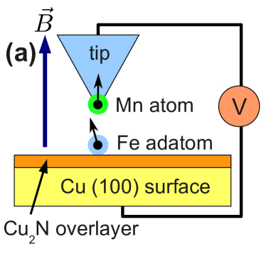
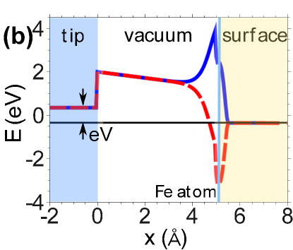
Figure 1: Color online (a) A spin-polarized STM tip is placed above a single Fe adatom adsorbed on the copper (100) surface with an Cu₂N overlayer to excite and probe the spin dynamics of the adatom. The tip consists of one Mn atom attached at the end of a tungsten tip. The Mn atom acts as a spin filter for the electrons propagating from the tip to the sample. A strong magnetic field of $B=7$ T adjusts the spin projection of the Fe atom nearly parallel to the spin polarization direction of the tip. (b) A theoretical model of (a) by a tunneling barrier and a spin-dependent interaction potential around the Fe atom on the surface. The solid line corresponds to the surface-deposited ground state spin. The coupling between surface-deposited spin and tip-spin states is antiferromagnetic. Hence, the coupling energy decreases when exciting the Fe spin states. The effective tunneling barrier for the first excited spin state is indicated by the dashed line.

Our model Hamiltonian matching the experimental situation in figure 1 includes

$$H_{0}=\frac{p^{2}}{2m}+V_{\mathrm{B}}+B\mu_{\mathrm{B}}\tau_{z},$$ (1)

which describes the tunneling electrons (with a mass $m$ and momentum operator $p$) emanating from the tip and are subject to the magnetic field $B$. They are coupled to the surface spin subsystem via a spin-dependent term $V_{\mathrm{B}}$. The spin of the tip electrons is described by the vector operators $\hat{\tau}=(\tau_{x},\tau_{y},\tau_{z})$ containing the Pauli matrices in their standard representation. In a similar way, $\hat{S}=(S_{x},S_{y},S_{z})$ are the operators for the surface spin. The tunneling barrier $V_{\mathrm{B}}(x)$ is measured relative to the Fermi levels of the tip or the sample (for simplicity we assume both to be equal). The last term in equation (1) describes the spin of the tip electrons in the presence of the magnetic field $B$.

The second subsystem is the surface spin in an anisotropic environment (due to the broken translational symmetry and other atoms placed nearby). The appropriate Hamiltonian for this part reads molecularmagnets1 ; surfacehamiltonian

$$H_{\mathrm{S}}=g\mu_{\mathrm{B}}BS_{z}+\delta S^{2}_{z}+\varepsilon(S^{2}_{x}-S^{2}_{y}),$$ (2)

which indicates that the easy axis is parallel to the (strong) magnetic field. We have chosen typical values for a rather strong magnetic anisotropy. This does not directly resemble the experimental situation, but serves to illustrate the effects arising from the anisotropic environment more clearly. In particular, we take $\delta\approx-5$ meV and $\varepsilon\approx 1.5$ meV for the anisotropy constants. The value of the magnetic field is kept with 7 T. The Landé factor $g$ is experimentally surfacehamiltonian found to be approximately 2, which corresponds to the total spin of the free Fe atom ($S=2$). The Hamiltonian (2) has 5 eigenstates $|\chi_{\nu}\rangle$ with eigenenergies $E^{S}_{\nu}$ (table 1 lists their properties). The ground state in orbital representation is depicted in figure 2.

Table 1: The spectrum of the adsorbate spin Hamiltonian (2), referred to the ground state, and the projection of the spin along the magnetic field. The third column contains the quantum number of $|m\rangle$ states with the dominant contributions to $|\chi_{\nu}\rangle$; the values are given in the last column.

$\nu$	$E^{S}_{\nu}-E^{S}_{1}$ (meV)	$\langle\chi_{\nu}|S_{z}|\chi_{\nu}\rangle$	$m$	$|\langle m|\chi_{\nu}\rangle|^{2}$
1	$0$	$-1.507$	$-2$	$0.855$
2	$2.006$	$1.498$	$2$	$0.869$
3	$12.121$	$-0.088$	$-1$	$0.544$
4	$21.156$	$0.088$	$1$	$0.544$
5	$22.901$	$0.009$	$0$	$0.944$

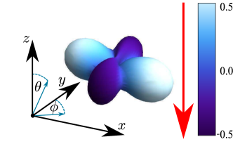
Figure 2: The ground state $\chi_{1}(\theta,\phi)$ in orbital representation. The shape is given by $|\chi_{1}(\theta,\phi)|$, whereas the color encodes the real part of the wave function. The red arrow denotes the expectation value of the spin $\langle\vec{S}\rangle$.

The third term on the left side in equation (2) results in a mixing of the different eigenstates $|m\rangle$ of the free spin in the magnetic field. Thus, the expectation value $\langle S_{z}\rangle$ in the ground state deviates from the noninteracting value -2. The ground state contains a large amount of free spin configurations (see table 1). The first excited state corresponds to the spin pointing in the opposite direction. Hence, the relaxation $|\chi_{2}\rangle\rightarrow|\chi_{1}\rangle$ is dominated by the transitions $|m=+2\rangle\rightarrow|m=-2\rangle$.

For the spin-dependent interaction of the tunneling electrons with the adsorbate we adopt the picture of extended states (tunneling electrons) coupled to a localized magnetic moment. In brief, such a process is known to be determined by the Hunds rules and the local electronic correlation. E.g. for $s$ states (with energy $\epsilon_{k}$) coupled to a pinned magnetic impurity (with energy $\epsilon_{d}$) one may utilize the Anderson model anderson : $H_{\mathrm{And}}=\sum_{k,\sigma}\epsilon_{k}n_{k\sigma}+\sum_{\sigma}\epsilon_{d}n_{d\sigma}+Un_{d\uparrow}n_{d\downarrow}+H_{\mathrm{ds}}$, where $\sigma$ labels the spins and $n_{k\sigma}$ ($n_{k\sigma}$) is the corresponding particle density operator. $U$ stands for the Coulomb repulsion between electrons with antiparallel spins. The term $H_{\mathrm{ds}}=\sum_{k,\sigma}V_{kd}c^{\dagger}_{k\sigma}c_{d\sigma}+\text{h.c.}$ accounts for the $s\mathchar 45\relax d$ hybridization with the mixing matrix element $V_{kd}$. The Anderson Hamiltonian is a model for a delocalized $s$-band interacting with a single $d$-orbital. As we are interested in the quantum dynamics of the local magnetic impurity we should map the Anderson model onto the Kondo Hamiltonian andersonkondo ($H_{\mathrm{Kondo}}=-J\hat{\sigma}_{s}\cdot\hat{\sigma}_{d}$) with the effective Kondo coupling constant $J$. Tunneling electrons in the vicinity of the Fermi level are of relevance for the tunneling. This leads to estimate $J=2|V_{k_{F}d}|^{2}\frac{U}{\epsilon_{d}(\epsilon_{d}+U)}<0.$ Typical values kondoeffect are in the order of $|V_{k_{F}d}|^{2}\approx 2$ eV, $U\approx 8$ eV and $\epsilon_{d}\approx 5$ eV, meaning that $J\approx 1$ eV.

In STM experiments the tip-sample distance (we take $5$ Å) is usually not negligible to the typical extent of $d$-orbitals in Fe adatoms (which is about $1$ Å). In the calculations, we use therefore an interaction $H_{\mathrm{int}}$ of the Kondo type with a spatial-dependent Kondo coupling

$$H_{\mathrm{int}}=u_{0}w(x)\hat{\tau}\cdot\hat{S}.$$ (3)

The $u_{0}>0$ is the coupling strength and the function $w(x)$ is a dimensionless form factor defining the width of the interaction region. We choose a strongly localized function with a width about $1$ Å.

The total Hamiltonain of the system is thus

$$H=H_{0}+H_{\mathrm{S}}+H_{\mathrm{int}}.$$ (4)

The total effective potential experienced by the tunneling electrons $V_{\mathrm{B}}(x)+\langle\chi_{\nu},\uparrow|H_{\mathrm{int}}|\chi_{\nu},\uparrow\rangle$ is thus different for the ground state $\nu=1$ and the first excited state $\nu=2$, as sketched in figure 1 (b) (the tip spin is $\uparrow$ in both cases). The anti-ferromagnetic coupling of the tip spin and the surface spin effectively raises the tunneling barrier for the tip electrons, for they have to overcome the additional spin-interaction energy. On the other hand, any excitation of the surface spin lowers the effective potential barrier (c. f. solid and dashed lines in figure 1 (b)). Therefore the excitation $|\chi_{1}\rangle\rightarrow|\chi_{2}\rangle$ is favored as long as the applied voltage is higher than the first excitation energy, i. e. if $eV>E^{S}_{2}-E^{S}_{1}$. For a smaller voltage this excitation is not reached energetically. All higher excited states also lower the effective potential barrier, but the effect is maximal for $|\chi_{2}\rangle$. This is reflected in the enhanced excitation probability for the first excited state.

If we on the other hand consider the case of $|\!\downarrow\rangle$-electrons beeing emitted from the tip, the effective potential $V_{\mathrm{B}}(x)+\langle\chi_{\nu},\downarrow|H_{\mathrm{int}}|\chi_{\nu},\downarrow\rangle$ undergoes a change of the sign in the last term. Therefore, $\langle\chi_{1},\downarrow|H_{\mathrm{int}}|\chi_{1},\downarrow\rangle$ becomes a negative contribution and thus enhances the tunneling current, whereas $\langle\chi_{2},\downarrow|H_{\mathrm{int}}|\chi_{2},\downarrow\rangle$ acts as an additional barrier. The other consequence is the smaller excitation probability because the transition $|\chi_{1}\rangle\rightarrow|\chi_{2}\rangle$ does not reduce the tunneling barrier. Physically, this picture reflects the anti-ferromagnetic coupling again.

We remark that the existence of a direct transition $|\chi_{1}\rangle\rightarrow|\chi_{2}\rangle$ is governed by the transition matrix element $\langle\chi_{\mu},\uparrow|H_{\mathrm{int}}|\chi_{\nu},\uparrow\rangle$ in the surface spin space, which is connected to the anisotropy constant $\varepsilon$. For the rather large value of $\varepsilon\approx 5$ meV, the direct excitation $|\chi_{1}\rangle\rightarrow|\chi_{2}\rangle$ is the dominant process epsdiscussion .

III Scattering formulation

In a wave-packet scattering picture of the process depicted in figure 1 one identifies an undisturbed part $H_{\mathrm{free}}=p^{2}/(2m)+g_{e}\mu_{\mathrm{B}}B\tau_{z}+H_{\mathrm{S}}$ and a scattering part $H_{\mathrm{sc}}=V_{\mathrm{B}}(x)+H_{\mathrm{int}}$. The unperturbed (asymptotic) scattering states are cast as ($\pm$ stand for incoming/outgoing waves) $|\Phi^{\pm}_{\nu,\tau}\rangle=|\pm k\rangle\otimes|\chi_{\nu}\rangle\otimes|\tau\rangle$ where $|\chi_{\nu}\rangle$ ($|\tau\rangle$) is the spin ground state of the surface (tip). $|\pm k\rangle$ is the orbital part of the wave with a wave vector $k$ which is determined by the direction and by the amplitude of the applied bias voltage $V$, i.e. $k=\sqrt{2meV/\hbar^{2}}$ (and $e$ is the electron charge). By propagating $|\Phi^{+}_{\nu,\tau}\rangle$ the state of the eigenstates $|\psi^{\pm}_{\nu,\tau}\rangle$ of the full Hamiltonian can be obtained (up to a phase)  scatteringtheory1 ; scatteringtheory2 ; gellmannlow , i.e. $|\psi^{+}_{\nu,\tau}\rangle=U(0,-\infty)|\Phi^{+}_{\nu,\tau}\rangle$ and $|\psi^{-}_{\nu,\tau}\rangle=U(+\infty,0)|\Phi^{-}_{\nu,\tau}\rangle$, where $U(t,t_{0})$ is the propagator in the interaction representation. Tunneling is governed by the probability amplitude to scatter from the incoming eigenstate $|\psi^{+}_{\mu,\sigma}\rangle$ into the outgoing state $|\psi^{-}_{\nu,\tau}\rangle$ is given by the scalar product $\langle\psi^{-}_{\nu,\tau}|\psi^{+}_{\mu,\sigma}\rangle=\langle\Phi^{-}_{\nu,\tau}|U(+\infty,-\infty)|\Phi^{+}_{\mu,\sigma}\rangle$. The last equation defines the on-shell S-matrix $S=U(+\infty,-\infty)$. Evaluating the S-matrix element

$$S^{\sigma\tau}_{\mu\nu}=\langle\Phi^{-}_{\nu,\tau}|S|\Phi^{+}_{\mu,\sigma}\rangle$$ (5)

we find the tunneling probability to scatter from the tip electron with a spin state $|\tau\rangle$ into $|\sigma\rangle$ and from the surface spin state $|\chi_{\nu}\rangle$ into $|\chi_{\mu}\rangle$ by taking the absolute value of the S-matrix (equation (5)). For a given initial spin-spin density matrix $\rho_{0}$ (of the dimension 10):

$$\rho_{0}=\rho^{tip}_{0}\otimes\rho^{S}_{0},$$

we obtain the total tunneling probability $T(V)$ and, thus, the normalized density matrix elements by

$$\rho^{\sigma\tau}_{\mu\nu}=\frac{1}{T(V)}\langle\Phi^{-}_{\nu,\tau}|U(+\infty,0)\rho_{0}U(0,-\infty)|\Phi^{+}_{\mu,\sigma}\rangle.$$ (6)

The probability to scatter into a specific channel $(\nu,\sigma)$ is given as

$$T_{\nu\tau}(V)=\langle\Phi^{-}_{\nu,\tau}|U(+\infty,0)\rho_{0}U(0,-\infty)|\Phi^{+}_{\nu,\tau}\rangle,$$ (7)

Whereas the total tunneling probability is $T(V)=\sum_{\nu,\tau}T_{\nu\tau}(V)=\text{Tr}\rho$.

In the setup figure 1 we are interested in the surface spin dynamics only. Hence, we trace out the spin $|\sigma\rangle$ of the tunneling tip electron. This yields the reduced density matrix of the surface spin. Furthermore, we fix the initial spin state of the tip electron as $|\tau\rangle=|\!\uparrow\rangle$ as determined by the polarization of the tip and $|\chi_{\nu}\rangle=|\chi_{1}\rangle$, i. e. the surface spin is in the ground state when we switch on the voltage. We simplify the notations and write the resulting density matrix as $\rho^{S}_{\mu\nu}$(V). The population of the final surface spin state $|\chi_{\nu}\rangle$ as a function of the applied voltage is then given by $P^{S}_{\nu}(V)=\rho^{S}_{\nu\nu}(V)$, whereas the phase information can be extracted from the off-diagonal elements.

The assumption $|\tau\rangle=|\uparrow\rangle$ corresponds to the case of a full polarization of the tip. A partial polarization $\beta$ can be included in the formalism via the initial spin density matrix of the tip, i.e.

$$\rho^{tip}_{0}=\frac{1}{2}\begin{pmatrix}1+\beta&0\\ 0&1-\beta\end{pmatrix}$$ (8)

For clarity however, we employ $\beta=1$ throughout this work and comment on the change of the results for $\beta<1$.

To calculate the individual S-matrix elements we utilize the wave packet approach wavepacket1 ; wavepacket2 . This method exploits the fact that in the Schrödinger picture the full eigenstates can be expressed as a superposition of propagated wave packets, i.e.

$$|\psi^{\pm}_{\nu,\tau}\rangle=\frac{1}{2\pi\hbar\eta^{\pm}_{\nu\tau}}\int^{\infty}_{-\infty}dt\ e^{-iHt/\hbar}e^{iEt/\hbar}|\phi^{\pm}_{\nu,\tau}\rangle,$$ (9)

where the normalization factor $\eta^{\pm}_{\nu\tau}$ is defined by

$$\eta^{\pm}_{\nu\tau}=\sqrt{\frac{m}{2\pi\hbar k}}\int^{\infty}_{-\infty}dx\ g_{\pm}(x)e^{ikx}.$$ (10)

The wave vector $k$ for $\eta^{+}_{\nu\tau}$, i. e. for the incoming waves, is given by $k=\sqrt{2meV/\hbar^{2}}$, whereas for the outgoing state, the wave vector may be reduced due to inelastic tunneling. In this case, we set $k=\sqrt{2m(eV+E^{S}_{1}+E^{\mathrm{tip}}_{\tau}-E^{S}_{\mu}-E^{\mathrm{tip}}_{\sigma})/\hbar^{2}}$ if the term under the square root is positive. Here $E^{\mathrm{tip}}_{\gamma}$ ($E^{S}_{\gamma}$) is the energy of the tip (surface) with a spin state $\gamma$.

The wave packets $|\phi^{\pm}_{\nu,\tau}\rangle$ are superpositions of full eigenstates. However, by placing the wave packets far away from the interaction region $U(t,t_{0})$ becomes the unit operator in which case the packets by composed of the eigenstates of $H_{\mathrm{free}}$, i. e. we can write $|\phi^{\pm}_{\nu\tau}\rangle$ as the product state $|g_{\pm}\rangle|\chi_{\nu}\rangle|\tau\rangle$ with a Gaussian function $g_{\pm}$. The subscripting $\pm$ now corresponds to centering the Gaussian to the left and to the right of the interaction region.

Using the spectral representation (equation 9) we find the S-matrix elements as

$$S^{\sigma\tau}_{\mu\nu}=\frac{1}{2\pi\hbar(\eta^{-}_{\mu})^{*}\eta^{+}_{\nu}}\int^{\infty}_{-\infty}dt\langle\phi^{-}_{\mu,\sigma}|e^{-iHt/\hbar}|\phi^{+}_{\nu,\tau}\rangle.$$ (11)

The formula (11) is then evaluated by (i) propagating the initial product state, (ii) calculating the overlap with the final state on the right side of the barrier, and (iii) by performing a Fourier transformation.

IV Spin state population

We now proceed with computing the population $P^{S}_{\nu}$ of the surface spin eigenstates $|\chi_{\nu}\rangle$ as a function of the applied voltage $V$ for different coupling constants $u_{0}$. We assume the surface spin to be initially in the ground state and the spin of the tip’s electron is being aligned with the magnetic field. Figure 3 depicts the dependence of the population of all surface spin states. The energy of the tunneling electrons ($eV$) determines which inelastic scattering processes are possible. For voltages below the excitation threshold the corresponding spin state can not be excited due to the energy conservation. For the other transitions, one has to take the spin of the tip’s electron into account, as well. By evaluating the spin-coupling $\hat{\tau}\cdot\hat{S}$ in the basis of product states one finds that the transitions $|\chi_{1}\rangle\rightarrow|\chi_{3}\rangle$ and $|\chi_{1}\rangle\rightarrow|\chi_{4}\rangle$ are only allowed if accompanied by spin flip processes. Other transitions require the conservation of the spin direction. We can, thus, define specific voltages $V_{\nu}$, where new tunneling channels open, i. e. $eV_{\nu}=E^{S}_{\nu}+E^{\mathrm{tip}}_{\sigma}-E^{\mathrm{tip}}_{\uparrow}-E^{S}_{1}$. For $\nu\neq 3,4$ we obtain $eV_{\nu}=E^{S}_{\nu}-E^{S}_{1}$ whereas for $\nu=3,4$ $eV_{\nu}=E^{S}_{\nu}+E^{\mathrm{tip}}_{\downarrow}-E^{\mathrm{tip}}_{\uparrow}-E^{S}_{1}$. The voltages $V_{\nu}$ are shown in figure 3 by vertical dashed lines.

The basic trend of the voltage-dependence of the population is to reduce the coupling energy by exciting the surface spin. As long as the energy of the tunneling electrons is high enough, the population of the ground state decreases. For voltages in the interval between the first two dashed lines, the first excited state is the only accessible tunneling channel, so that the population is solely transferred to $|\chi_{2}\rangle$. The efficiency of this transition is determined by the coupling constant $u_{0}$. If the voltage increases further, the next tunneling channels open and the spin interaction energy can again be lowered by exciting the surface spin. Therefore, $P^{S}_{2}$ decreases and $P^{S}_{3}$ rises by the same amount. The situation is similar between the last two dashed lines, where $P^{S}_{3}$ is decreased in order to increase $P^{S}_{4}$. The highest state $|\chi_{5}\rangle$ corresponds to a very small projection parallel to the magnetic field as the major contribution is $|m=0\rangle$ (see table 1). The transition probability is, thus, much smaller than a transition into the other states. For the surface spin it is therefore more convenient to maintain a higher population of $|\chi_{4}\rangle$ instead of decreasing $P^{S}_{4}$ when the voltage exceeds the last threshold.

For larger coupling constants $u_{0}$ the probability to scatter to the excited states of the surface spin increases. However, this holds true as long as $u_{0}<u^{c}_{0}$, where $u^{c}_{0}$ is about $7$ eV. For larger $u_{0}$, the transition efficiency decreases again. In order to reveal the dependence on $u_{0}$, we calculated the population of the ground state as a function of $V$ and $u_{0}$ (figure 4). Since the effects are especially pronounced for the transition $|\chi_{1}\rangle\rightarrow|\chi_{2}\rangle$, we will only consider the corresponding voltage interval. As it turns out, the excitation of the surface spin is only probable for certain values of the coupling constant. For large $u_{0}$, the excitation probability even approaches zero.

In order to explain this behavior, we have to apply a further simplification that renders possible an analytical treatment (see appendix). Analyzing the simplified model we infer that

$$u^{c}_{0}=\frac{\hbar^{2}q}{2mx_{0}C_{22}}$$ (12)

with $C_{22}=\langle\chi_{2}|S_{z}|\chi_{2}\rangle$ and $q=\sqrt{2mV_{B}/\hbar^{2}}$ for the optimal value of the coupling strength. Physically, the occurrence of this optimal value can simply be interpreted as a resonance phenomenon of scattering on the narrow quantum well of the spin-spin-interaction potential. The value of $u^{c}_{0}$ is represented by the horizontal white dashed line in figure 4.

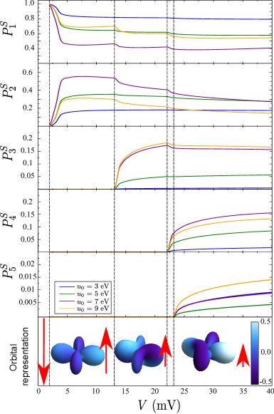
Figure 3: The population $P^{S}_{\nu}$ for all spin states of the surface-deposited structure as a function of the applied voltage for various coupling strengths $u_{0}$. The black dashed lines indicate when the voltage is high enough as to excite the surface-deposited spin states obeying the energy condition $E^{S}_{\nu}+E^{\mathrm{tip}}_{\sigma}-E^{\mathrm{tip}}_{\uparrow}-E^{S}_{1}-eV>0$. The bottom row depicts the voltage-dependent wave functions in orbital representation (for $u_{0}=7$ eV), evaluated for the highest voltage between two black dashed lines. The color coding is as in figure 2. The red arrow indicates the expectation value of the spin. Note that when exceeding the first threshold voltage, the spin direction flips, as it is primarily connected to the transition $|m=+2\rangle\rightarrow|m=-2\rangle$.

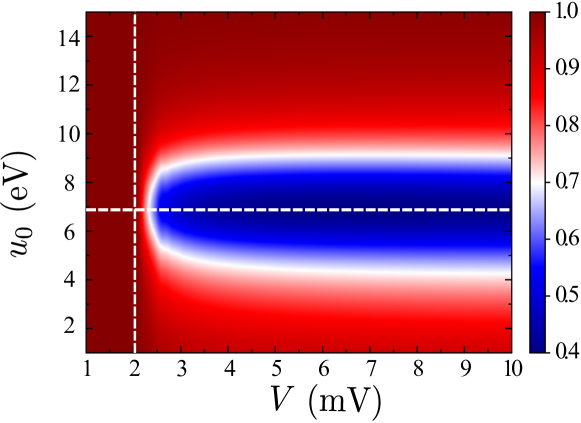
Figure 4: The population $P^{S}_{1}$ in the ground state as a function of the voltage $V$ and the coupling strength $u_{0}$. The voltage is bounded such that the only accessible tunneling channel is the first excited spin state of the adatom. the vertical white dashed line indicates the energy difference $E^{S}_{2}-E^{S}_{1}$. We find that the depopulation process of the ground state is particularly efficient for $u_{0}\approx 7$ eV. For stronger or weaker coupling strengths, the excitation probability decreases. This can be understood by a simple analytical model (see appendix). The prediction of this consideration for the optimal value $u^{c}_{0}$ is shown by the horizontal white dashed line.

Generally, for values for the tip polarization $\beta<1$, the excitation probability decreases. We have already noted that the transitions induced by the tunneling electrons with the opposite spin direction ($|\tau\rangle=|\!\downarrow\rangle$) are weaker in comparison to $|\!\uparrow\rangle$-electrons. For $\beta$ decreasing from $\beta=1$, the strong ($|\!\uparrow\rangle$) and the weak ($|\!\downarrow\rangle$) contribution are mixed together finitebeta . Despite from beeing reduced to a smaller intervall of the probability, the shape of the curves in figure 3 remains the same for realistic values of $\beta\approx 30$ %.

The resonance phenomenon arising from the quantum well of the effective potential becomes also less visible for a smaller tip polarization, as the quantum well is inverted to a barrier for electron spins of the opposite direction. The value of $u^{c}_{0}$ is however hardly influenced.

V Relaxation dynamics

STM experiments are not only suitable for determining the transport properties, but also offers an insight in the relaxation dynamics of the excited surface spin by using a pump-probe scheme. The time resolution is not sufficient to resolve the precession or the transitions between neighboring $|m\rangle$ states, but it is still high enough to measure the relaxation from $|m=+2\rangle$ to $|m=-2\rangle$. This corresponds in a good approximation to the transition $|\chi_{2}\rangle\rightarrow|\chi_{1}\rangle$.

The idea of determining the relaxation dynamics is to apply a pump voltage pulse in order to excite the surface spin, i. e. to increase the population $P^{S}_{2}$ and to detect the time evolution by a second probe pulse. The voltage of the latter has to be chosen according to the excitation threshold. We set the maximal values $V^{(0)}_{\mathrm{pump}}=3$ mV and $V^{(0)}_{\mathrm{probe}}=1$ mV. This specific value for the pump voltage is sufficient to induce an excitation of the adsorbate spin. If the excitation has to take place with the help of intermediate states, e. g. if the transition matrix element does not allow for the direct pathway $|\chi_{1}\rangle\rightarrow|\chi_{2}\rangle$, the pump voltage has to be chosen higher according to the energy of these intermediate states. We note that in our case the sum of $V^{(0)}_{\mathrm{pump}}$ and $V^{(0)}_{\mathrm{probe}}$ is much smaller than the voltage $V_{3}$ needed to excited the third or higher excited states. The tip spin can not flip for the transition $|\chi_{1}\rangle\rightarrow|\chi_{2}\rangle$, hence we can reduce our considerations to a two-level system (TLS).

The experimentally accessible quantity is the number of tunneling electron $N$ during the time interval containing the pump and the probe pulses shifted against each other by a time delay $\Delta t$ as displayed in figure 5.

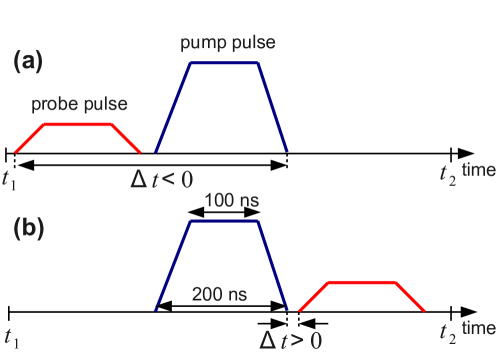
Figure 5: A sketch of the pump-probe arrangement of the voltage pulses. In the case (a) the probe pulse advances the pump pulse characterized by $\Delta t<0$ and the cross correlation of both pulses is zero. On the other hand, by varying $\Delta t>0$ as in (b) one can determine the relaxation time for the transition $|\chi_{2}\rangle\rightarrow|\chi_{1}\rangle$. The probe and the pump pulse both have a duration of $200$ ns with the linear rise/fall intervals of $50$ ns.

For large $|\Delta t|$ and $\Delta t<0$ (5a), there is no overlap of the pump and probe pulse. The number of tunneling electrons is therefore just the sum of the electrons transmitted during probe pulse $N_{\mathrm{probe}}$ and pump pulse $N_{\mathrm{pump}}$ separately. This number of electrons will be denotes as $N_{0}=N_{\mathrm{pump}}+N_{\mathrm{probe}}$. For smaller $|\Delta t|$ but still negative $\Delta t$, the pump and the probe pulse have a finite overlap, i. e. there is a certain time interval where the effective voltage is $V_{\mathrm{pump}}+V_{\mathrm{probe}}$. If the current-voltage characteristic is nonlinear, the $N$ will be different from $N_{0}$ because of the correlation of probe and pump pulse. In our case, the nonlinearity mainly arises from the coupling Hamiltonian $H_{\mathrm{int}}$.

For $\Delta t>0$ the pump and the probe pulses have again no overlap, but the pump pulse depletes the population of the ground state. The following probe pulse can only access the ground state scattering channel, hence the number of transmitted electrons is lower than $N_{0}$. With $\Delta t$ increasing, there is more time for the surface spin to relax back to the ground state, so $N$ approaches $N_{0}$ again for a large $\Delta t$.

For a quantitative analysis, we note that all quantities are only parametrically time-depended, since the time-dependence of $V_{\mathrm{pump}}(t)$ and $V_{\mathrm{probe}}(t)$ is very slow on the typical time scales of the system. This means we can use the results of the steady-state considerations from the section III and IV. From the tunneling probability for the different scattering channels $T_{\nu\sigma}(V)$ we compute the corresponding currents as $j_{1,2}=(e\hbar k_{1,2}/m)T_{(1,2)\uparrow}(V)$ with $k_{1}=\sqrt{2meV/\hbar^{2}}$ and $k_{2}=\sqrt{2m(eV+E^{S}_{1}-E^{S}_{2})/\hbar^{2}}$ for $eV>E^{S}_{2}-E^{S}_{1}$ and $k_{2}=0$ otherwise. The total current is expressed as the sum $j=j_{1}+j_{2}$ proportional to the total number of tunneling electrons $dN$ in the given time interval $dt$. As the calculations are based on the quasi-static regime, it is still possible to define the conductance $G(V)\propto dj/dV$, which then is parametrically time-dependent, as well. As we have pointed out in section IV, the excitation of the state $|\chi_{2}\rangle$ is favored as long as the voltage is sufficiently high. For this reason, the average slope of $j_{2}(V)$ is larger than the average slope of $j_{1}(V)$, i. e. the conductance jumps to a higher value if $eV$ exceeds $E^{S}_{2}-E^{S}_{1}$. The nonlinear conductance profile is depicted in figure 6.

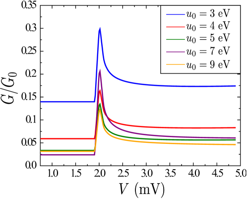
Figure 6: The conductance of the magnetic tunneling junction for various coupling strengths $u_{0}$. The value of $G$ has been normalized to the situation where $u_{0}=0$, in which case the conductance is almost constant.

We note the population of the ground state and the first excited state evolve only adiabatically with resultant voltage $V_{\mathrm{pump}}(t)+V_{\mathrm{probe}}(t)$, because the excitation $|\chi_{1}\rangle\rightarrow|\chi_{2}\rangle$ occurs instantly on the time scale of the voltage pulses. With the surface spin driven into the excited state, it undergoes i) a precession (the characteristic time is about 2 ps) and ii) relaxes. Since the computation of $N$ involves an integration over the time interval of several hundred nanoseconds, the oscillatory part due to the precession does not play a role. We can, therefore, describe the dynamics of the surface spin in the case of a falling voltage by using the Bloch equations including damping, but at a zero frequency. The time scale for this relaxation process, chosen according to the experiment experiment , is again very slow for our system.

For a pump-probe delay $\Delta t<0$ such that the probe pulse still advances the pump pulse, we therefore obtain

$$N=\frac{1}{eL}\int dt~{}j(V_{\mathrm{pump}}(t)+V_{\mathrm{probe}}(t))$$ (13)

with $j(V)=e\hbar(k_{1}T_{1\uparrow}(V)+k_{2}T_{2\uparrow}(V))/m$. For $\Delta t>0$ on the other hand, there is no overlap of the two pulses and hence the number of electrons transmitted due to the pump pulse is given by $N_{\mathrm{pump}}=\frac{1}{eL}\int dt~{}j(V_{\mathrm{pump}}(t))$. The probe pulse can only access the ground state $|\chi_{1}\rangle$. The tunneling probability and equivalently the current are in this case proportional to the population $P^{S}_{1}$, which we obtain by calculating $P^{S}_{1}(V^{(0)}_{\mathrm{pump}}+V^{(0)}_{\mathrm{probe}})<1$ and then computing the increase of $P^{S}_{1}(t)$ back to 1 due to the relaxation. The number of tunneling electrons due to the probe pulse $N_{\mathrm{probe}}=\frac{1}{eL}\int dt~{}P^{S}_{1}(t)j_{1}(V_{\mathrm{probe}}(t))$ is, thus, lowered in comparison to the probe pulse advancing the pump pulse.

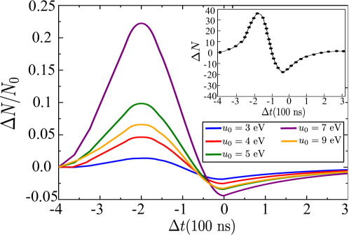
Figure 7: The relative number of the transmitted electrons with respect to $N_{0}$ as a function of the delay $\Delta t$ of pump and probe pulses for various interaction strengths $u_{0}$. The curve has a peak at $\Delta t=-200$ ns which refers to a complete overlap of the probe and the pump pulses. Since the population in the ground state is lowered by the excitation of the surface spin, $N-N_{0}$ becomes negative for $\Delta t>0$ and approaches zero again when the excited state relaxes back into the ground state. Our calculations, thus, confirm that threshold phenomena may also arise under different excitations: $|\chi_{2}\rangle$ is excited directly. For comparison, the inset shows the experimental result from Ref. experiment, where the same final state is reached by a sequence of excitations with $\Delta m=1$.

Figure 7 shows the total dependence of $N$ on the time delay $\Delta t$. Again the curves in figure 7 evidence a strong dependence on the coupling of the tunneling electron to the local moment $u_{0}$. The peak at $\Delta t=-200$ ns (corresponding to a complete overlap of the pump and the probe pulses) is due to the nonlinearity of current-voltage characteristic, as $j(V^{(0)}_{\mathrm{pump}}+V^{(0)}_{\mathrm{probe}})>j(V^{(0)}_{\mathrm{pump}})+j(V^{(0)}_{\mathrm{probe}})$. The magnitude of this effect can be explained by means of the the conductance profile (figure 6). For small values of $u_{0}$, the relative jump of the conductance is small, so $j(V)$ is nearly linear, i. e. $j(V_{\mathrm{pump}}(t)+V_{\mathrm{probe}}(t))\gtrsim j(V^{(0)}_{\mathrm{pump}})+j(V^{(0)}_{\mathrm{probe}})$. Hence, $N$ only slightly exceeds $N_{0}$ when both pulses coincide. For this reason, the first peak in figure 7 is small for smaller $u_{0}$. The maximum becomes more pronounced when approaching the optimal value of $u_{0}$ for the depopulation of the ground state. From the conductance profile (figure 6) we conclude that the relative jump of $G$ when exceeding the threshold voltage attains the highest value for $u_{0}=u^{c}_{0}$. The nonlinearity then plays a dominant role, resulting in an especially strong increase of $N$ with respect to $N_{0}$. For larger coupling strength, the current-voltage dependence resembles again the linear case. Note that the averaged conductance is much smaller for $u_{0}>u^{c}_{0}$ than in the case $u_{0}<u^{c}_{0}$. The minimum at $\Delta t=0$ is caused by the reduction of the ground state population $P^{S}_{1}$ due to the advancing pump pulse. We have already discussed the efficiency of this process (figure 4). For values $u_{0}\ll u^{c}_{0}$ or $u_{0}\gg u^{c}_{0}$, $P^{S}_{1}\lesssim 1$ holds. Hence, $N_{\mathrm{probe}}$ and for this matter $N$ decrease only by a small amount. The depth of the minimum is maximal for $u_{0}=u^{c}_{0}$.

We remark that the relative jump in the conductance profile also decreases for $\beta<1$. The tunneling channel connected to the excitation $|\chi_{1}\rangle\rightarrow|\chi_{2}\rangle$ is much less effective for $|\!\downarrow\rangle$-electrons emitted from the tip. Hence, the major contribution for this electrons arises from the adsorbate spin remaining in the ground state. Hence, the conductance for voltages $eV>E^{S}_{2}-E^{S}_{1}$ differs only slightly from the value left to this threshold. This effect again shows a linear dependence on the tip polarization. The total value of the conductance on the other hand increases with smaller $\beta$, which is due to the reduction of the effective potential for $|\!\downarrow\rangle$-electrons with the adsorbate spin in the ground state.

Similarly to the discussion in section IV, the special features with respect to $u^{c}_{0}$ become less visible if we reduce $\beta$. Hence, the height of maximum in figure 7 decreases. This can be explained in terms of the conduction profile which more and more resembles the linear case. On the other hand, the transition of the surface spin to the first excited state effectively blocks the $|\!\downarrow\rangle$-electrons from the tips and therefore reduces the current more than in the case $\beta=1$. We thus conclude that the minimum becomes deeper for a realistic tip polarization.

VI Conclusions

We analyzed theoretically the dynamics of a surface-deposited localized magnetic moment, triggered by a spin-polarized current pulse from an STM tip in the presence of a magnetic field. We showed and explained how and why the spin population of the surface-deposited structure can be manipulated by applying appropriate voltages and investigated the dependence on the coupling strength $u_{0}$ of the tunneling electrons to the localized moments. A simplified analytical model allowed us to predict a value of $u_{0}$ for which the excitation probability of the surface spin is particularly high. The obtained value is in excellent agreement with the numerical calculations.

The relaxation was incorporated by using the Bloch equations, as our model does not provide a relaxation mechanism. For future work, this point deserves a special consideration. In this respect, the main advantage of the Cu₂N-overcoat is the magnetic decoupling of the adatom and the substrate, the excitation of magnons is strongly suppressed leading to prolonged relaxation times. In general, we suggest the spin-orbit interaction, that transfers the energy to the substrate, as the major dissipation channel.

The above treatment is based on an adiabatic approximation in the sense, that the voltage pulses durations are very long on the time scale of the electron and spin dynamics, which is a very well justified assumption for the experiments under consideration (figure 1). In future experiments one may envisage however to go beyond the relaxation dynamics with the aim to image the precession of the adsorbate spin as well. In this case picosecond pulses are required. Such pulses have already been utilized for tracing the ultrafast spin dynamics in a proof of principle experiments slac1 ; slac2 . Alternatively, one may consider laser-pulse induced tunneling currents, as in the recent experiments atto ; atto2 . Generally, the characteristic times for the tunneling process (some femtoseconds) and the spin dynamics (picoseconds) are still very different. Hence, the dynamics driven by the voltage pulses with picosecond durations can be adiabatically decomposed into (i) the time evolution of the electron states, (ii) the electron pulse driving the surface spin, and (iii) an adiabatic dependence of the current on the surface-deposited spin dynamics (which images of the spin dynamics). This time scale separation is the key for future experiments and calculations on road to full insight into the spatiotemporal evolution of the quantum spin dynamics.

VII Appendix: Analytical model

In section IV that for the parameters of interest the excitation probability exhibits a maximum for $u_{0}\approx 7$ eV. To explain the specific value of the maximum and to gain further insight in the underlying physics, we introduce here some reasonable simplifications that allow an analytically solvable model. Since the scattering channels are limited to the first two states of the surface-deposited magnetic moment and the tip electron spin can not flip within this transition, we can reduce our considerations to a two-channel model. The operator $\hat{\tau}\cdot\hat{S}$ can be replaced by $S_{z}$ as the electron spin is fixed in the $z$-direction. For small voltages, the gradient of the potential barrier can be neglected. We can, thus, assume a rectangular shape of the barrier. The function $w(x)$ describing the spin-interaction area is localized around the Fe atom. Hence we approximate the coupling Hamiltonian by

$$H_{\mathrm{int}}=u_{0}C~{}\delta\left(\frac{x-L}{x_{0}}\right),$$ (14)

where $x_{0}$ is a typical length associated with $w(x)$, $L$ is the width of the vacuum barrier and $C$ is the remaining coupling matrix that contains the transition amplitudes, i. e. $C_{\alpha\beta}=\langle\chi_{\alpha}|S_{z}|\chi_{\beta}\rangle$.

The wave functions $\psi^{+}_{\nu}(x)$ are then linear combinations of plane waves $e^{\pm ik(x-L)}$ for $x<0$ or $x>L$ and $e^{\pm q(x-L)}$ for $x\in(0,L)$. The respective wave vector follows as $k_{\nu}=\sqrt{2m(eV+E^{S}_{1}-E^{S}_{\nu})/\hbar^{2}}$, whereas $q_{\nu}=\sqrt{2m(V_{B}-eV-E^{S}_{1}+E^{S}_{\nu})/\hbar^{2}}$. Since the height of the vacuum barrier $V_{B}$ is much greater than the electron energy, we can approximately set $q_{\nu}=q=\sqrt{2mV_{B}/\hbar^{2}}$. For $0<x<L$ we write $\psi^{+}_{\nu}(x)=\alpha^{<}_{\nu}e^{qx}+\beta^{<}_{\nu}e^{-qx}$ and for $x>L$ we define $\psi^{+}_{\nu}(x)=\alpha^{>}_{\nu}e^{ik_{\nu}x}+\beta^{>}_{\nu}e^{-ik_{\nu}x}$. The coefficients are linked by the corresponding transfer matrices. Imposing the standard matching conditions for the wave-function and its derivative we obtain for the reflection coefficient of the first excited spin state in the interval $(0,L)$:

$$\beta^{<}_{2}=-\alpha^{>}_{1}\frac{m}{\hbar^{2}}\frac{x_{0}u_{0}C_{12}}{q}+\alpha^{>}_{2}\left(\frac{ik_{2}}{2q}+\frac{\hbar^{2}q-2mx_{0}u_{0}C_{22}}{2\hbar^{2}q}\right),$$ (15)

where $>$ and $<$ labels the coefficients to the left and to the right of $x=L$. We can furthermore neglect the term $k_{2}/q$ because of the small voltages. The remaining terms are then real, so that the absolute value of $\beta^{<}_{2}$ is minimal if the right side in equation (15) is minimal. Hence, $\alpha^{>}_{1}$ becomes small near the optimal value $u^{c}_{0}$. We conclude that $\beta^{<}_{2}$ is small for $q=2mx_{0}u_{0}C_{22}/\hbar^{2}$, yielding for the optimal value $u^{c}_{0}=\hbar^{2}q/(2mx_{0}C_{22})$.

- (1) Wolf S A, Awschalom D D, Buhrman R A, Daughton J M, von Molnàr S, Roukes M L, Chtchelkanova A Y and Treger D M 2001 Science 294 1488
- (2) Chappert C, Fert A and Van Dau F N 2007 Nat. Mater. 6 813
- (3) Léger Y, Besombes L, Fernández-Rossier J, Maingault L and Mariette H 2006 Phys. Rev. Lett. 97 107401
- (4) Awschalom D D and Flatte M E 2007 Nat. Phys. 3 153
- (5) Gatteschi D, Sessoli R and Villain J 2006 Molecular nanomagnets (New York: Oxford University Press)
- (6) Bogani L and Wernsdorfer W 2008 Nat. Mater. 7 179
- (7) Ardavan A, Rival O, Morton J J L, Blundell S J, Tyryshkin A M, Timco G A and Winpenny R E P 2007 Phys. Rev. Lett. 98 057201
- (8) Loth S, Etzkorn M, Lutz C P, Eigler D M and Heinrich A J 2010 Science 329 1628
- (9) Loth S, Baumann S, Lutz C P, Eigler D M and Heinrich A J 2012 Science 335 196
- (10) Sloan P A 2010 J. Phys.: Condens. Matter 22 264001
- (11) Recher P, Sukhorukov E V and Loss D 2000 Phys. Rev. Lett. 85(3) 1962
- (12) Delgado F and Fernández-Rossier J 2011 Phys. Rev. B. 84(3) 045439
- (13) Penteado P H, Souza F M abd Seridonio A C abd Vernek E and Egues J C 2011 Phys. Rev. B. 84(3) 125439
- (14) Hirjibehedin C F, Lin C Y, Otte A F, Ternes M, Lutz C P, Jones B A and Heinrich A J 2007 Science 317 1199
- (15) Anderson P W 1966 Phys. Rev. Lett. 17 95
- (16) Schrieffer J R and Wolff P A 1966 Phys. Rev. 149 491
- (17) Calvo M R, Fernández-Rossier J, Palacios J J, Jacob D and Natelson D 2009 Nature 458 1150
- (18) By evaluating the transition element , we found that the direct excitation to the first excited state is always possible for . Furthermore, the direct pathway turns out to be very efficient for the parameters used in this work. This changes if the value of decreases, i. e. becomes very small, so that stepwise excitations over intermediate states start to dominate.
- (19) Joachain C J 1975 Quantum Collision Theory (Amsterdam: North-Holland Publishing Company)
- (20) Goldberger M L and Watson K M 1967 Collision Theory (New York: Wiley)
- (21) Gell-Mann M and Goldberger M L 1953 Phys. Rev. 91 398
- (22) Tannor D J and Weeks D E 1993 J. Chem. Phys. 98 3884
- (23) Grossmann F 2004 Phys. Rev. B 70 113306
- (24) One can readily show that the population of the eigenstates of change according to when taking a finite tip spin polarization into account. This formula connects the probabilities with the initial condition for in a linear way.
- (25) Weber W, Riesen S and Siegmann H C 2001 Science 291 1015
- (26) Gamble S J, Burkhard M H, Kashuba A, Allenspach R, Parkin S S P, Siegmann H C and Stöhr J 2006 Phys. Rev. Lett. 102(3) 217201
- (27) Takeuchi O and Shigekawa H 2005 Springer Series in Optical Science 99(3) 285
- (28) Terada Y, Yoshida S, Takeuchi O and Shigekawa H 2005 Nat. Phot. 4(12) 869