Cluster-formation in the Rosette molecular cloud at the junctions of filaments

Abstract

Aims. For many years feedback processes generated by OB-stars in molecular clouds, including expanding ionization fronts, stellar winds, or UV-radiation, have been proposed to trigger subsequent star formation. However, hydrodynamic models including radiation and gravity show that UV-illumination has little or no impact on the global dynamical evolution of the cloud. Instead, gravitational collapse of filaments and/or merging of filamentary structures can lead to building up dense high-mass star-forming clumps. However, the overall density structure of the cloud has a large influence on this process, and requires a better understanding.

Methods. The Rosette molecular cloud, irradiated by the NGC 2244 cluster, is a template region for triggered star-formation, and we investigated its spatial and density structure by applying a curvelet analysis, a filament-tracing algorithm (DisPerSE), and probability density functions (PDFs) on Herschel column density maps, obtained within the HOBYS key program.

Results. The analysis reveals not only the filamentary structure of the cloud but also that all known infrared clusters except one lie at junctions of filaments, as predicted by turbulence simulations. The PDFs of sub-regions in the cloud show systematic differences. The two UV-exposed regions have a double-peaked PDF we interprete as caused by shock compression, while the PDFs of the center and other cloud parts are more complex, partly with a power-law tail. A deviation of the log-normal PDF form occurs at A_V$\approx$9^m for the center, and around 4^m for the other regions. Only the part of the cloud farthest from the Rosette nebula shows a log-normal PDF.

Conclusions. The deviations of the PDF from the log-normal shape typically associated with low- and high-mass star-forming regions at A_V$\approx$3–4^m and 8–10^m, respectively, are found here within the very same cloud. This shows that there is no fundamental difference in the density structure of low- and high-mass star-forming regions. We conclude that star-formation in Rosette – and probably in high-mass star-forming clouds in general – is not globally triggered by the impact of UV-radiation. Moreover, star formation takes place in filaments that arose from the primordial turbulent structure built up during the formation of the cloud. Clusters form at filament mergers, but star formation can be locally induced in the direct interaction zone between an expanding H II-region and the molecular cloud.

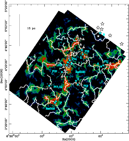
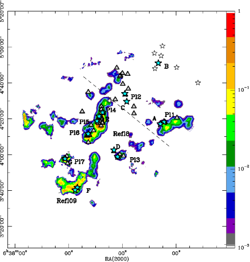
Figure 1: Left: Curvelet map of the column density, expressed in logarithmic magnitudes of visual extinction (A_V= 0.05 to 7). The absolute values, however, depend on the decomposition threshold ($\approx$20% of the intensity are in the curvelets) and are not relevant for this study. The filamentary structure becomes apparent and is additionally traced by DisPerSE (white lines). See Appendix B for more details and a close-up of the central region. Known infrared-clusters are indicated as blue stars (’Pl’ for Phelps & Lada phelps1997 (1997), A–F for Poulton et al. poulton2008 (2008), and Refl for Román-Zúñiga et al. 2008). White stars in the upper right corner indicate the O-stars from NGC 2244. Gray triangles are the massive dense cores (MDCs) identified in Motte et al. (motte2010 (2010)). Right: A map showing the ’confidence’ (coded from 0 to 1 in color scale) of finding cluster formation sites. This map combines the information of the column density map and the locations of filament junctions (see text for details). Known clusters and MDCs are labeled as in the left panel. The dashed line indicates the approximate border beyond which (toward the cluster) SF due to the direct compression scenario may be at work.

1 Introduction

The role of feedback from massive stars has been long discussed as a dynamical trigger for subsequent star formation (SF). One has to distinguish, however, between the driving scales on which the processes work – and their relative importance. Large-scale turbulence, even on a Galactic scale (Mac Low & Klessen maclow2004 (2004)), can be excited by expanding supernova shells, colliding flows forming clouds, or globally by any form of accretion (Klessen & Hennebelle klessen2010 (2010)). Intermediate- to small-scale processes include radiation, stellar winds, and outflows. Observationally, expanding ionization fronts were proposed to account for fragmented shells around bubble-like H II-regions (e.g. Zavagno et al. zavagno2010 (2010)). Shock compression of a simple layer is the initial idea of the collect and collapse scenario (Elmegreen & Lada elmlada1977 (1977)). Recent models (Walch et al. walch2011 (2011)) consider now an initially inhomogeneous cloud. In particular Dale & Bonnell (dale2011 (2011), dale2012 (2012)) showed that photoionizing radiation from an OB-cluster on a spatially highly inhomogeneous molecular cloud has little or no impact on the global evolution of the cloud due to the presence of strong accretion flows. Generally, in a dynamic view of molecular cloud- and SF-interactions (e.g., Ballesteros-Paredes et al. ball2007 (2007)), stars form in gravitationally collapsing dense filaments that formed in turbulence-generated, interacting shocks. Dale & Bonnell (dale2011 (2011)) proposed that the most massive clusters should be found at the junctions of filaments. This confirms the finding of Schneider et al. (2010a) where a mass flow through subfilaments, probably governed by magnetic fields, was observed for the DR21 filament. The prediction that (massive) clusters form preferentially in the deep potential wells where filaments merge can be verified observationally and it is within the scope of this paper to do so. We chose the Rosette Molecular cloud (RMC) as a proposed template for ’triggered’ SF. A discussion of the advantages and disadvantages of this premise can be found in Schneider et al. (2010b). To characterize the cloud structure, a curvelet decomposition of column density maps obtained with Herschel data is performed, and a filament-tracing algorithm is applied to the map (see Arzoumanian et al. 2011 and Appendix B for details).
The Rosette nebula at a distance of 1.6 kpc is illuminated by the central OB cluster NGC~2244 located inside a cavity. The expanding H II-region is interacting with a GMC (mass of a few $10^{5}\leavevmode\nobreak\ {\rm M}_{\odot}$, Williams et al. williams1995 (1995)). Photon dominated regions (PDRs) are detected not only along the interface but also deep inside the molecular cloud (Schneider et al. schneider1998 (1998)), reflecting the deep penetration of UV-radiation owing to its inhomogenous structure. We investigated the density structure of the RMC by deriving probability density functions (PDFs) of the column density of the whole cloud and subfields in the Rosette. To do this, we used observations from Herschel within the HOBYS (Herschel imaging survey of OB Young Stellar objects, Motte, Zavagno, Bontemps et al. 2010) guaranteed time key program. Column density maps were determined from a modified black body fit to the wavelengths of PACS and SPIRE (see Appendix A) and have an angular resolution of $\approx$37^′′. Generally, a PDF characterizes the fraction of gas that has a column density $N$ in the range [$N$, $N$+$\Delta N$] (e.g., Federrath et al. fed2008 (2008)).

2 Results and analysis

2.1 The filamentary structure of Rosette

Figure 1 (left) shows a curvelet image from a multi-resolution morphological decomposition (Starck et al. starck2004 (2004)) of the column density map of the Rosette (see Fig. 2) obtained from Herschel data. Overlaid on the image are the filaments traced by the DisPerSE algorithm (Sousbie et al. sousbie2011 (2011)). This method reveals the highly filamentary structure of the RMC, which is not fully apparent from visual inspection of the column density map (or molecular line maps). Existing infrared (IR) clusters and the most massive dense cores (MDCs) identified in the same data set (Motte et al. 2010; Hennemann et al. hennemann2010 (2010)) are overlaid on the image. The latter are potential sites of future massive star formation. It is apparent that all sources lie in the proximity of junctions of the most prominent filaments in high column density regions. Some of the MDCs and the cluster Pl2, however, are also located along filaments (see, e.g., close-up of the center region shown in Fig. 5). To better qualitatively characterize the filament-junction/cluster correlation, we created a ’confidence map’ that combines the two requirements for cluster formation: high column density and filament junction. First, we produced a mask containing only the junction points and then defined a Gaussian distribution function with a FWHM of 3^′=1.5 pc around each point. This procedure yields a ’junction-area’ that is more realistic than only a single point. We then multiplied this map with the column density map, and normalized the resulting map to obtain values between 0 and 1. Inspection of Fig. 1 (right) shows that the IR-clusters and many MDCs are indeed found in regions of high column density where filaments merge (all within the maximum cluster size of 7 pc). The only exception is the H II-region/molecular cloud interface (northwest of the dashed line in Fig. 1). Neither cluster Pl2 nor the majority of MDCs lie in regions of high confidence. Here, shock compression of the expanding ionization front with subsequent fragmentation into dense cores may be at work, as suggested by the PDFs of this region (see next Sec. 2.2).

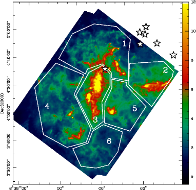
Figure 2: Column density map of the Rosette molecular cloud, expressed in visual extinction (see color bar). The six regions that were selected to determine individual PDFs are indicated by polygons.

2.2 PDFs from the Herschel column density map of Rosette

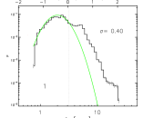
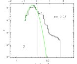
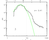
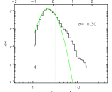
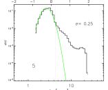
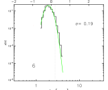
Figure 3: PDFs for the six subregions in the Rosette, labeled from 1 to 6. The green line indicates the fitted PDF. The A_V -value of the deviation of the PDF from the log-normal form is shown as a dotted vertical line and the width of the PDF ($\sigma_{\eta}$) is given in each panel.

Figure 2 shows the column density map including our division into several subregions, reflecting different morphological and physical properties. (1) and (2): interface of H II-region and molecular cloud with many UV-exposed pillars, (3): dense, main SF region of the RMC, including several IR-clusters (Pl4/5/6), (4) and (5): more diffuse and colder gas with dense, SF clumps (Pl7 in region 4 and Pl3 in region 5), (6): quiescent and cold remote part of the cloud without SF activity.

The PDF obtained for the whole molecular cloud is displayed in Appendix C (Fig. 6). A log-normal PDF with a width of $\sigma_{\eta}$=0.63 is fitted up to A_V =3^m (noise level $\approx$1^m). The excess at high column densities (A_V =3–20^m) follows a power law. The slope corresponds to a volumetric, radial density profile of $n\propto r^{-0.65}$ (Federrath et al. fed2011 (2011)). This does not assume that the cloud is a single sphere, moreover it consists of many clumps/cores, each with a radial profile leading to a common exponent $\alpha$. The exponent is smaller than what is typically found for dense cores (–1.5 to –2), suggesting that on large (cloud)-scales, turbulence is the dominating process compared to gravity.

Figure 3 displays the PDFs for the six subregions, all showing a log-normal distribution at low A_V  and a more complex curvature or several peaks at higher A_V. Particularly interesting are the PDFs of the UV-exposed regions 1 and 2 (the OB-cluster is only 10–15 pc away in projected distance) because there are two ’peaks’ (at A_V$\approx$3^m and 6^m). A similar double-peak PDF was observed (Schneider et al., priv. comm.) using a column density map of RCW120 (Zavagno et al. 2010), a very good example of a simple, ’bubble’-like geometry. We interpret the second peak as arising from a higher column density component due to gas compression by the expanding ionization front. This interpretation is supported by recent numerical models including turbulence and radiation (Tremblin et al., in prep.) that exhibit double-peak PDFs depending on the turbulent state of the cloud and the initial curvature of the cloud surface. We therefore do not expect to see this feature in all UV-illuminated environments. Region 3 is the central SF region with the highest column density (up to 70^m). The PDF here is broad ($\sigma_{\eta}$=0.41), shows two ’breaks’ (around 9^m and 20^m), and has a peak value at A_V $\approx$5^m (all other PDFs peak at $\approx$2^m). The PDFs of regions 4 and 5 cover a lower density regime and deviate from the log-normal form around A_V $\approx$4^m. The most quiescent region 6 is the only one displaying a well-defined log-normal PDF with the smallest width ($\sigma_{\eta}$=0.19).

3 Discussion

3.1 The density structure of the RMC

In Csengeri et al. (in prep.), we found that low-mass SF regions have a break in the log-normal shaped PDF at A_V $\approx$4^m (and possibly around 8^m), and high-mass SF regions around A_V $\approx$8^m and higher. We now show that these two breaks in A_V  are found in the PDFs of subregions within one single cloud, the Rosette GMC, suggesting that there is no fundamental difference in the density structure of low-mass and high-mass SF regions up to an A_V  of typically 7–10^m. Above this value, the tail(s) in the PDFs are associated with SF activity. Namely, if gravity starts to play a role during molecular cloud formation, an increasing fraction of gas will exceed a certain threshold of column density/extinction and form stars. Other studies (e.g., Lada et al. lada2010 (2010); Heiderman et al. heider2010 (2010); André et al., 2010) have arrived at the same value of around 8^m. In addition, only numerical models that include gravity are able to reproduce this threshold and the corresponding break in the PDF. For example, Ballesteros-Paredes et al. (2011) showed that PDFs vary during cloud evolution. Purely log-normal shapes were found in an initially turbulent, non-gravitating cloud, while one or more log-normal PDFs at low column-densities and a power-law tail for higher values were found for later stages of cloud evolution. In addition, the slope of the power-law tails varies with time. All PDFs in the Rosette have the shape of the later evolutionary states, indicating that gravity remains an important process in cloud evolution, including star-formation. The impact of UV radiation, however, needs to be investigated using hydrodynamic simulations including gravity and radiation.

3.2 Where do stars form ?

Our Rosette observations indicate that clusters preferentially form at filament junctions but cores (and subsequently stars) can also form along filaments (see also other studies of high-mass SF regions, e.g., the Nessie-nebula (Jackson et al. jackson2010 (2010)), W48 (Nguyen Luong et al. quang2011 (2011)) or Cygnus (Motte et al. motte2007 (2007))). In Herschel observations of low-mass SF regions (André et al. andre2010 (2010); Arzoumanian et al. doris2011 (2011)) dense cores were found to be located along super-critical filaments without higher concentrations at the junctions. This points toward a scenario in which it is the large potential well of merging filaments (subcritical or supercritical) that enables the formation of massive stars within a cluster. Conform with numerical simulations (e.g. Klessen & Hennebelle klessen2010 (2010); Vázquez-Semadeni et al. vaz2009 (2009)) it is therefore ultimately the total mass and the high accretion rate that is the decisive factor for the formation of a cluster. Observationally, apart from the present study, there are more examples of how massive structures can be built up from parsec-scale filaments (DR21, Schneider et al. 2010a and Hennemann et al., in prep.; Vela C, Hill et al. 2011). The supply of material may continue on much smaller (subparsec) scales to build-up a cluster with massive stars, as proposed by, e.g., Csengeri et al. (csengeri2011 (2011)). Alternatively, massive stars may form in a turbulence-regulated, quasi-static scenario (McKee & Tan tan2003 (2003)). However, the discussion of these small, subparsec scale processes is beyond the scope of this paper.

3.3 Does triggered star-formation exist ?

Dale & Bonnell (2011, 2012) simulated the gravitational collapse of a turbulent (giant) molecular cloud exposed to photoionizing radiation. Their main conclusion was that although the gas and dust is heated, photoionization has no strong global, i.e. tens of parsec scale, effect on the dense gas because the massive clumps out of which OB clusters form are continuously accreting and most of the photoionizing flux is absorbed by these accretion flows. Observationally, no clear picture emerges. In the RMC, a very low UV-field in the remote part of the cloud was determined ($\approx$2-8 Habing at a distance of 30 pc, Schneider et al. 1998), supporting the idea of low UV-impact. On the other hand, a temperature gradient, and a tentative age-gradient of sources, was derived (Schneider et al. 2010b). In addition, local triggering of SF, as seen in the RMC (and RCW36, Minier et al., in prep.) is possible (Sec. 2.1). The observed double-peak PDFs (Sec. 2.2) support this scenario. We therefore conclude that though the morphological and PDF analysis of Rosette shows no evidence that SF is globally triggered (across the whole extent of the cloud), but is moreover governed by gravity, the impact of UV-radition is not settled and needs more investigation.

Appendix A Observations and column density map

4

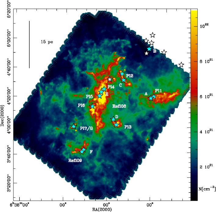
Figure 4: Column density map of the Rosette Molecular Cloud, obtained from the 160, 250, 350, and 500 $\mu$m maps from Herschel. Known infrared-clusters are indicated in the plot as blue stars (’Pl’ refers to Phelps & Lada (phelps1997 (1997)), A, B, etc. the clusters from Poulton et al. (poulton2008 (2008)), and labeling “Refl” those from Román-Zúñiga et al. (2008)). White stars in the upper right corner indicate the O-stars from NGC2244.

The Rosette was observed during the Science Demonstration Phase (SDP) within the HOBYS key program. This program is dedicated to the earliest stages of high-mass star formation and images all molecular complexes that form high-mass stars at less than 3 kpc with SPIRE (Griffin et al. griffin2010 (2010)) and PACS (Poglitch et al. poglitsch2010 (2010)) using the Herschel satellite (Pilbratt et al. pilbratt2010 (2010)). The SPIRE and PACS data from 70 $\mu$m to 500 $\mu$m were obtained on October 20, 2009 in parallel mode with a scanning speed of 20^′′/sec. Two orthogonal coverages of size 1^∘45${}^{\prime}\times$1^∘25^′ were performed, mapping the (largest) southeast part of the Rosette Molecular Cloud. The SPIRE data were reduced with HIPE version 7.1956, using a modified version of the pipeline scripts, i.e., observations that were taken during the turnaround at the map borders were included, the most recent calibration tree was used, and the destriper-module with a polynomial baseline of 0th order was applied. The two orthogonally scanned maps were then combined using the ‘naive-mapper’ (i.e., a simple averaging algorithm). The destriper module significantly improved the resulting maps, compared to the first data reduction just after the SDP (Schneider et al. 2010b). The angular resolutions at 160, 250, 350, and 500 $\mu$m, are $\sim$12^′′, $\sim$18^′′, $\sim$25^′′, and $\sim$37^′′, respectively.

The column density was determined from a pixel-to-pixel modified black body fit to four wavelengths of PACS and SPIRE (160, 250, 350, 500 $\mu$m, all maps were smoothed to the beamsize of the 500 $\mu$m map, i.e., $\sim$37^′′). For the region covered by PACS and SPIRE simultaneously, we fixed the specific dust opacity per unit mass (dust+gas) approximated by the power law $\kappa_{\nu}\,=\,0.1\,(\nu/1000GHz)^{\beta}$ cm²/g and $\beta$=2, and left the dust temperature and column density as free parameters (see Hill et al. 2011; Arzoumanian et al. 2011 for details). For the region only covered with SPIRE we used 17.3 K, the median value of the SED-derived temperature across the main map where PACS and SPIRE overlap giving us four-band coverage at 160, 250, 350, and 500 $\mu$m. We checked the fitted SEDs and found no major discrepancy in the fits, though the method described above assumes a single temperature and optically thin emission, which is not always a good approximation if there is a temperature variation along the line-of-sight, noise, and if the dust becomes optically thick at shorter wavelengths. Shetty et al. (shetty2009 (2009)), for example, showed that this can even produce an anti-correlation of $\beta$ and T which was claimed to be observed by other authors. However, it is beyound the scope of this paper to go more into detail. While the column density map shown in Schneider et al. (2010b) was calibrated using extinction maps, we now recovered the Herschel zero-flux levels of the Rosette field with Planck data (Bernard et al., priv. communication). The final column density map is shown in Fig. 4.

5

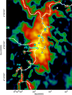
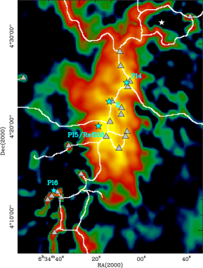
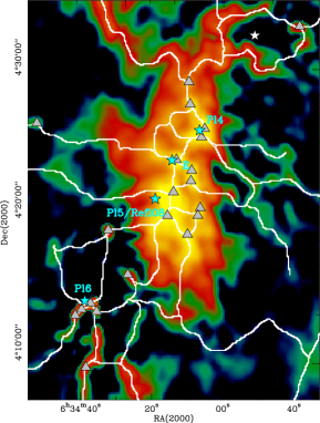
Figure 5: Close-up of the curvelet image (Fig. 1) of the center region of the Rosette molecular cloud with the filamentary structure traced by DisPerSE, indicated with white lines. Different thresholds (called ’persistence’, i.e. intensity contrast level, for filament detection were used (2.9, 1.0, 0.5$\times$10²¹ cm^-2 from left to right). The curvelet image has a maximum value for the column density of 2$\times$10²² cm^-2 with a sigma of 0.5$\times$10²¹ and the original column density map a maximum of 9.4$\times$10²² cm^-2 with a sigma of 1.4$\times$10²¹.

Appendix B Curvelet/wavelet decomposition and filament tracing

There are two parameters determining the detection of filaments: First, the seperation into curvelets and wavelets, and second the threshold of DisPerSE to detect filaments. From our experience on the curvelet/wavelet analysis from Herschel column density maps so far (André et al. 2010; Arzoumanian et al. 2011; Hill et al. 2011), and from several tests with Rosette, we arrived at a good compromise of 20% of the intensity being in the curvelets (a difference of around $\pm$10%, however, does not change the overall picture). This reveals the filamentary structure without completely suppressing the more compact sources. The DisPerSE algorithm detects filaments starting from a given threshold (defined as difference between saddle points and peak values) on the curvelet image. However, the column density map is a 2D-projection of the volume density while DisPerSE works topologically, connecting all emission features such that projection effects may create links between filaments that are not physically related. To overcome this caveat, filament tracing using molecular line data cubes can be a solution, as first tests on the DR21 filament have shown (Schneider et al., in prep.).

Figure 5 shows as an example a close-up of the crowded center region of Rosette where different thresholds were applied. A threshold is defined by an intensity contrast between pixels, the lowest one starting at 0.5$\times$10²¹ cm^-2 and accordingly finding many filaments, up to to a fairly conservative value of 2.9$\times$10²¹ cm^-2, leaving only the most prominent features. For this paper, a threshold of 1.0$\times$10²¹ cm^-2 was choosen in order not to detect too faint filaments. It is only the most prominent ones that are able to provide enough material that is accreted onto the cluster center to build up high enough masses. Again, changing the threshold does not alter these prominent filaments, they always remain detected.

Appendix C Probability density function of the Rosette cloud

The probability density function of the whole cloud obtained from the column density map (Fig. 2 or 4) is shown in Fig. 6 in linear and logarithmic scaling. It displays a log-normal form for lower column densities and a clearly defined power-law tail for higher column densities that was fitted with a power-law. This is not generally the case, while the PDF of the high-mass SF region NGC6334 also shows a clear power-law tail (Russeil et al., in prep.), the PDFs of other high-mass SF clouds are more complex and show several breaks in the PDFs (Hill et al. 2011, Csengeri et al., in prep.). The reason for that can partly be line-of-sight effects and limited angular resolution. A more detailed disussion of PDFs of intermediate- and high-mass SF regions and comparison to models is presented in Csengeri et al. (in prep.).

6

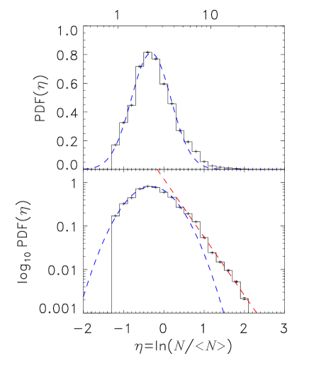
Figure 6: Probability density function of the whole cloud obtained from the column density map in linear (top) and logarithmic (bottom) scaling. The upper labeling indicates the visual extinction. The red dashed line shows a power-law fit (the high-density range beyond A_V =20^m is not well resolved, we therefore do not attempt to fit a second power law.)