Pulse-front tilt caused by the use of a grating monochromator and self-seeding of soft X-ray FELs

Abstract

Self-seeding is a promising approach to significantly narrow the SASE bandwidth of XFELs to produce nearly transform-limited pulses. The development of such schemes in the soft X-ray wavelength range necessarily involves gratings as dispersive elements. These introduce, in general, a pulse-front tilt, which is directly proportional to the angular dispersion. Pulse-front tilt may easily lead to a seed signal decrease by a factor two or more. Suggestions on how to minimize the pulse-front tilt effect in the self-seeding setup are given.

DEUTSCHES ELEKTRONEN-SYNCHROTRON

Ein Forschungszentrum der Helmholtz-Gemeinschaft

DESY 12-051

March 2012

Pulse-front tilt caused by the use of a grating monochromator and self-seeding of soft X-ray FELs

Gianluca Geloni,

European XFEL GmbH, Hamburg

Vitali Kocharyan and Evgeni Saldin

Deutsches Elektronen-Synchrotron DESY, Hamburg ISSN 0418-9833 NOTKESTRASSE 85 - 22607 HAMBURG

1 Introduction

As a consequence of the start-up from shot noise, the longitudinal coherence of X-ray SASE FELs is rather poor compared to conventional optical lasers. Self-seeding schemes have been studied to reduce the bandwidth of SASE X-ray FELs SELF -OURS . In general, a self-seeding setup consists of two undulators separated by a photon monochromator and an electron bypass, normally a four-dipole chicane. For soft X-ray self-seeding , a monochromator usually consists of a grating SELF . Recently, a very compact soft X-ray self-seeding scheme has appeared, based on grating monochromator FENG , FENG2 .

In OURS we studied the performance of this compact scheme for the European XFEL upgrade. Limitations on the performance of the self-seeding scheme related with aberrations and spatial quality of the seed beam have been extensively discussed in FENG , FENG2 and go beyond the scope of this paper. Here we will focus our attention on the spatiotemporal distortions of the X-ray seed pulse. Numerical results provided by ray-tracing algorithms applied to grating design programs give accurate information on the spatial properties of the imaging optical system of grating monochromator. However, in the case of self-seeding, the spatiotemporal deformation of the seeded X-ray optical pulses is not negligible: aside from the conventional aberrations, distortions as pulse-front tilt should also be considered WEIN , HEBL , PRET . The propagation and distortion of X-ray pulses in grating monochromators can be described using a wave optical theory. Most of our calculations are, in principle, straightforward applications of conventional ultrafast pulse optics WEIN . Our paper provides physical understanding of the self-seeding setup with a grating monochromator, and we expect that this study can be useful in the design stage of self-seeding setups.

2 Theoretical background for the analysis of pulse-front tilt phenomena

2.1 Pulse-front tilt from gratings

Figure 1: Schematic representation of the electric field profile of an undistorted pulse beam (left) and of a beam with pulse front tilt (right). The z axis is along the beam propagation direction (adapted from PRET ).

Figure 2: Geometry of diffraction grating scattering.

Ultrashort X-ray FEL pulses are usually represented as products of electric field factors separately dependent on space and time. The assumption of separability of the spatial (or spatial frequency) dependence of the pulse from the temporal (or temporal frequency) dependence is usually made for the sake of simplicity. However, when the manipulation of ultrashort X-ray pulses requires the introduction of coupling between spatial and temporal frequency coordinates, such assumption fails. The direction of energy flow -usually identified as rays directions- is always orthogonal to the surface of constant phase, that is to the wavefronts of the corresponding propagating wave. If one deals with ultrashort X-ray pulses, one has to consider, in addition, planes of constant intensity, that is pulse fronts. Fig. 1 shows a schematic representation of the electric field profile of an undistorted pulse and one with a pulse-front tilt. A distortion of the pulse front does not affect propagation, because the phase fronts remain unaffected. However, for most applications, including self-seeding applications, it is desirable that these fronts be parallel to the phase fronts, and therefore orthogonal to the propagating direction.

A pulse-front tilt can be present in the beam due to the propagation through a grating monochromator. As shown in Fig. 2, the input beam is incident on the grating at an angle $\theta_{i}$. The diffracted angle $\theta_{D}$ is a function of frequency, according to the well-known plane grating equation. Assuming diffraction into the first order, one has

$$\lambda=d(\cos\theta_{i}-\cos\theta_{D})~{},$$ (3)

where $\lambda=2\pi c/\omega$, and $d$ is the groove spacing. Eq. (3) describes the basic working of a grating monochromator. By differentiating this equation one obtains

$$\frac{d\theta_{D}}{d\lambda}=\frac{1}{\theta_{D}d}~{},$$ (4)

where we assume grazing incidence geometry, $\theta_{i}\ll 1$ and $\theta_{D}\ll 1$. The physical meaning of Eq. (4) is that different spectral components of the outcoming pulse travel in different directions. The electric field of a pulse including angular dispersion can be expressed in the Fourier domain $\{k_{x},\omega\}$ as $E(k_{x}-p\omega,\omega)$, while the inverse Fourier transform from the $\{k_{x},\omega\}$ domain to the space-time domain $\{x,t\}$ can be expressed as $E(x,t+px)$, which is the electric field of a pulse with a pulse-front tilt. The tilt angle $\gamma$ is given by $\tan\gamma=cp$. More specifically

$$p=\frac{dk_{x}}{d\omega}=k\frac{d\theta_{D}}{d\omega}=\frac{\lambda}{c}\frac{d\theta_{D}}{d\lambda}=\frac{\lambda}{c\theta_{D}d}~{}.$$ (5)

Therefore one concludes that the pulse-front tilt is invariably accompanied by angular dispersion. It follows that any device like a grating monochromator, that introduces an angular dispersion, also introduces significant pulse-front tile, which is problematic for seeding.

2.2 Spatiotemporal transformation of X-ray FEL pulses by crystals

The development of self-seeding schemes in the hard X-ray wavelength range necessarily involves crystal monochromators. Recently, the spatiotemporal coupling in the electric field relevant to self-seeding schemes with crystal monochromators has been analyzed in the frame of classical dynamical theory of X-ray diffraction SHVID . This analysis shows that a crystal in Bragg reflection geometry transforms the incident electric field $E(x,t)$ in the $\{x,t\}$ domain into $E(x-at,t)$, that is the field of a pulse with a less well-known distortion, first studied in GABO . The physical meaning of this distortion is that the beam spot size is independent of time, but the beam central position changes as the pulse evolves in time. One of the aims of this subsection is to disentangle what is specific to the transformation by a crystal and what is intrinsic to the grating case. Our purpose here is not that of presenting novel results but, rather, to attempt a more intuitive explanation of spatiotemporal coupling phenomena in the dynamical theory of X-ray diffraction, and to convey the importance and simplicity of the results presented in SHVID .

Figure 3: Reflection of the primary beam from the lattice planes in the crystal according to Bragg law.

We begin our analysis by specifying the scattering geometry under study. The angle between the physical surface of the crystal and the reflecting atomic planes is an important factor. The reflection is said to be symmetric if the surface normal is perpendicular to the reflecting planes in the case of Bragg geometry. We shell examine only the symmetric Bragg case, Fig. 3.

Let us consider an electromagnetic plane wave in the X-ray frequency range incident on an infinite, perfect crystal. Within the kinematical approximation, according to the Bragg law, constructive interference of waves scattered from the crystal occurs if the angle of incidence, $\theta_{i}$ and the wavelength, $\lambda$, are related by the well-known relation

$$\lambda=2d\sin\theta_{i}~{}.$$ (6)

assuming reflection into the first order. This equation shows that for a given wavelength of the X-ray beam, diffraction is possible only at certain angles determined by the interplanar spacings $d$. It is important to remember the following geometrical relationships:

1. The angle between the incident X-ray beam and normal to the reflection plane is equal to that between the normal and the diffracted X-ray beam. In other words, Bragg reflection is a mirror reflection, and the incident angle is equal to the diffracted angle ($\theta_{i}=\theta_{D}$).

2. The angle between the diffracted X-ray beam and the transmitted one is always $2\theta_{i}$. In other words, incident beam and forward diffracted (i.e. transmitted) beam have the same direction.

We now turn our attention beyond the kinematical approximation to the dynamical theory of X-ray diffraction by a crystal. An optical element inserted into the X-ray beam is supposed to modify some properties of the beam as its width, its divergence, or its spectral bandwidth. It is useful to describe the modification of the beam by means of a transfer function. The reflectivity curve - the reflectance - in Bragg geometry can be expressed in the frame of dynamical theory as

$$R(\theta_{i},\omega)=R(\Delta\omega+\omega_{B}\Delta\theta\cot\theta_{B})~{},$$ (7)

where $\Delta\omega=(\omega-\omega_{B})$ and $\Delta\theta=(\theta_{i}-\theta_{B})$ are the deviations of frequency and incident angle of the incoming beam from the Bragg frequency and Bragg angle, respectively. The frequency $\omega_{B}$ and the angle $\theta_{B}$ are given by the Bragg law: $\omega_{B}\sin\theta_{B}=\pi c/d$. We follow the usual procedure of expanding $\omega$ in a Taylor series about $\omega_{B}$, so that

$$\omega=\omega_{B}+(d\omega/d\theta)_{B}(\theta-\theta_{B})+...~{}.$$ (8)

Consider a perfectly collimated, white beam incident on the crystal. In kinematical approximation $R$ is a Dirac $\delta$-function, which is simply represented by the differential form of Bragg law:

$$d\lambda/d\theta_{i}=\lambda\cot\theta_{i}~{}.$$ (9)

In contrast to this, in dynamical theory the reflectivity width is finite. This means that there is a reflected beam even when incident angle and wavelength of the incoming beam are not related exactly by Bragg equation. It is interesting to note that the geometrical relationships 1. and 2. are still valid in the framework of dynamical theory. In particular, reflection in dynamical theory is always a mirror reflection. We underline here that if we have a perfectly collimated, white incident beam, we also have a perfectly collimated reflected beam. Its bandwidth is related with the width of the reflectivity curve. We will regard the beam as perfectly collimated when the angular spread of the beam is much smaller than the angular width of the transfer function $R$. It should be realized that the crystal does not introduce an angular dispersion similar to a grating or a prism. However, a more detailed analysis based on the expression for the reflectivity, Eq. (7), shows that a less well-known spatiotemporal coupling exists. The fact that the reflectivity is invariant under angle and frequency transformations obeying

$$\Delta\omega+\omega_{B}\Delta\theta\cot\theta_{B}=\mathrm{const}~{}$$ (10)

is evident, and corresponds to the coupling in the Fourier domain $\{k_{x},\omega\}$. The origin of this relation is kinematical, it is due to Bragg diffraction. One might be surprised that the field transformation derived in SHVID for an XFEL pulse after a crystal in the $\{x,t\}$ domain is given by

$$E_{\mathrm{out}}(x,t)=FT[R(\Delta\omega,k_{x})E_{\mathrm{in}}(\Delta\omega,k_{x})]=E(x-ct\cot\theta_{B},t)~{},$$ (11)

where $FT$ indicates a Fourier transform from the $\{k_{x},\omega\}$ to the $\{x,t\}$ domain, and $k_{x}=\omega_{B}\Delta\theta/c$. In general, one would indeed expect the transformation to be symmetric in both the $\{k_{x},\omega\}$ and in the $\{x,t\}$ domain due to the symmetry of the transfer function. However, it is reasonable to expect the influence of a nonsymmetric input beam distribution. In the self-seeding case, the incoming XFEL beam is well collimated, meaning that its angular spread is a few times smaller than angular width of the transfer function. Only the bandwidth of the incoming beam is much wider than the bandwidth of the transfer function. In this limit, we can approximate the transfer function in the expression for the inverse temporal Fourier transform as a Dirac $\delta$-function. This gives

$$E_{\mathrm{out}}(x,t)=FT[R(\Delta\omega,k_{x})E_{\mathrm{in}}(\Delta\omega,k_{x})]$$ (12)

$$=\xi(t)\cdot\frac{1}{2\pi}\int dk_{x}\exp(-ik_{x}ct\cot\theta_{B})\exp(ik_{x}x)E_{\mathrm{in}}(0,k_{x})$$ (13)

$$=\xi(t)b(x-ct\cot\theta_{B})~{},$$ (14)

where we applied the Shift Theorem twice, and where

$$\xi(W)=\frac{1}{2\pi}\int dY\exp(iYW)R(Y)$$ (15)

is the inverse Fourier transform of the reflectivity curve.

In the opposite limit when the incoming beam has a wide angular width and a narrow bandwidth we take the transfer function in the inverse spatial Fourier transform as a Dirac $\delta$-function. This gives

$$E_{\mathrm{out}}(x,t)=\xi(x\tan\theta_{B}/c)a(t-(x/c)\tan\theta_{B})~{},$$ (16)

where $\xi(x)$ is given in Eq. (15). These two limits represent the two sides of the symmetry of the transfer function.

The last expression, Eq. (16) is the field of a pulse with a pulse front tilt. Typically one would think that a pulse front tilt can be introduced only by dispersive elements like gratings or prisms. Here we presented an example in which no dispersive elements exists, and we stress that angular dispersion can be introduced by non dispersive element like crystals too.

Although we began by considering a case of reflection transfer function in Bragg reflection geometry, none of our arguments depends on that fact. Eq. (7) still holds if the transfer function R is referred to the transmittance in Bragg reflection geometry. For the transmitted beam, all derivations are worked out in the same way we have done here and gives asymptotic expression like Eq(14) , Eq. (16) for field of forward scattered pulses.

3 Modeling of self-seeding setup with grating monochromator

A self-seeding setup should be compact enough to fit one undulator segment. In this case its installation does not perturb the undulator focusing system and allows for the safe return to the baseline mode of operation. The design adopted for the LCLS is the novel one by Y. Feng et al. FENG , FENG2 , and is based on a planar VLS grating. It is equipped only with an exit slit. Such design includes four optical elements, a cylindrical and spherical focusing mirrors, a VLS grating and a plane mirror in front of the grating. The optical layout of the monochromator is schematically shown in Fig. 4.

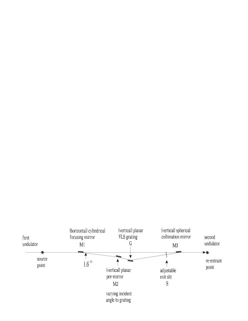
Figure 4: Optics for the compact grating monochromator originally proposed at SLAC FENG , FENG2 for the soft X-ray self-seeding setup.

Figure 5: Diagram of the self-seeding grating monochromator used in theoretical analysis. For simplicity the grating is depicted in transmission mode, and tilt is not shown. The dashed lines refer to different planes at which the field is calculated (adapted from WEIN ).

A simplified diagram for analyzing the grating monochromator is shown in Fig. 5. We will assume that the optical system used for imaging purposes is the well-known two-lens image formation system. With reference to Fig. 4, the VLS grating is represented by a combination of a planar grating with fixed line spacing and a lens, with the focal length of the lens equal to the focal length of the VLS grating. The analysis of the grating monochromator is simplified by recognizing that the grating can be shifted from a position immediately before the lens to a position immediately after the object plane. The monochromator is treated assuming no aberrations. This approximation is useful, since for the design shown on Fig. 4 the aberration effects are negligible FENG , FENG2 . This simplifies calculations and allows analytical results to be derived.

The angular dispersion of the grating causes a separation of different optical frequencies at the Fourier plane of the first focusing element (lens). Therefore, this system becomes a tunable frequency filter if a slit is placed at the Fourier plane. We assume that the two lenses in Fig. 5 are not identical, so that this scheme allows for magnification by changing the focal distance of the second lens.

It is important to analyze the output field from the grating monochromator quantitatively. In our analysis we calculate the propagation of the input signal to different planes of interest within the self-seeding monochromator, as indicated in Fig. 5. We start by writing the input field in plane 1, immediately before the grating, as

$$E_{1}(x,t)=\mathrm{Re}[a(t)b(x)\exp(i\omega_{0}t)]~{},$$ (17)

where $\omega_{0}$ is the pulse carrier frequency, which is linked to $k$ by $k=\omega_{0}/c$. We assume that the input signal is Gaussian in the transverse direction, that is $b(x)=1/\left(\sqrt{2\pi}\sigma\right)\exp(-x^{2}/2\sigma^{2})$. The field in plane 2, immediately after the grating (assuming diffraction into the first order) may be written as

$$E_{2}(x,t)=\frac{\sqrt{\beta}}{2\pi}\mathrm{Re}\int d\Delta\omega A(\Delta\omega)b(\beta x)\exp(ip\Delta\omega x)\exp[i\omega t],$$ (18)

where the astigmatism factor $\beta=\theta_{i}/\theta_{D}$, results due to the difference in input and output angles, and $p=\lambda/(c\theta_{D}d)$.

Our analysis exploits the Fourier transform properties of a lens. In particular we consider the propagation of a monochromatic one-dimensional field in paraxial approximation. The field distribution in the focal plane of the first lens, which we call plane 3, is given by

$$E_{3}(x,t)=\frac{1}{2\pi\sqrt{\lambda f\beta}}\mathrm{Re}\int d\Delta\omega\sqrt{i}A(\Delta\omega)\hat{b}\left(\frac{k}{\beta f}(x+\eta\Delta\omega)\right)\exp(i\omega t)~{},$$ (19)

where $\hat{b}(k_{x})$ refers to the spatial Fourier transform of the input spatial profile, $\eta=f\lambda^{2}/(2\pi cd\theta_{D})$ is a spatial dispersion parameter, which describes the proportionality between spatial displacement and optical frequency. In the case of a Gaussian input beam we have $\hat{b}(k_{x})=\exp(-\sigma^{2}k_{x}^{2}/2)$. Therefore, the field in the Fourier plane is written as

$$E_{3}(x,t)=\frac{1}{2\pi\sqrt{\lambda f\beta}}\mathrm{Re}\int d\Delta\omega\sqrt{i}A(\Delta\omega)\exp\left[-\frac{(x+\eta\Delta\omega)^{2}}{2\sigma_{f}^{2}}\right]\exp(i\omega t)~{},$$ (20)

(21)

where $\sigma_{f}=\beta f/(k\sigma)$ is the rms of the focused beam at the Fourier plane for any single frequency component.

We now add a slit at the Fourier plane, that we regard as a particular spatial mask with a real transmission function $S(x)$. The field in plane 4, that is directly after the slit is simply given by

$$E_{4}(x,t)=S(x)E_{3}(x,t)~{}.$$ (22)

Let us first consider the limiting case of a $\delta$-function slit that is, physically, a slit with much narrower opening than the spot size of a fixed individual frequency, centered at transverse position $x^{\prime}$. For a Gaussian input beam, the square modulus of the transmittance of the monochromator, that is the frequency response, is given by

$$|T(\Delta\omega)|^{2}=A_{0}\exp\left[-\left(\frac{\lambda\sigma}{cd\theta_{i}}\right)^{2}(\Delta\omega-\Delta\omega^{\prime})^{2}\right]~{}.$$ (23)

The center frequency of the passband , $\Delta\omega^{\prime}=x^{\prime}/\eta$, is determined by the transverse position of the slit. The spectral resolution of the monochromator depends on the spot size at the Fourier plane related with the individual frequencies, $\sigma_{f}$, and on the rate of spatial dispersion with respect to the frequency (determined by $\eta$). The FWHM of the monochromator spectral line is

$$\frac{\Delta\omega}{\omega}=1.18\frac{d\theta_{i}}{2\pi\sigma}\sim\frac{1}{\pi N}~{},$$ (24)

where $N\sim 2\sigma/(d\theta_{i})$ is the number of grooves illuminated by the input beam. For any single frequency the spot size at the Fourier plane, and hence the bandwidth transmitted through a narrow slit, is inversely proportional to the input spot size. Since the temporal spread in the output pulse is inversely proportional to the transmitted bandwidth, the output pulse duration is proportional to the input spot size.

To get to the plane prior to the second undulator entrance, that will be called plane 5, we simply perform a second spatial Fourier transform. The resulting field is located at an output plane at distance $f^{\prime}$ behind the second lens with focal distance $f^{\prime}$, and is given by

$$E_{5}(x,t)=\frac{1}{2\pi\lambda\sqrt{f^{\prime}f\beta}}\mathrm{Re}\int d\Delta\omega~{}iA(\Delta\omega)\exp(i\omega t)$$ (25)

$$\times\int\int dx^{\prime}dx^{\prime\prime}S(x^{\prime\prime})b(x^{\prime})\exp\left[\frac{ikx^{\prime}(x^{\prime\prime}+\eta\Delta\omega)}{\beta f}\right]\exp\left(\frac{ikxx^{\prime\prime}}{f^{\prime}}\right)$$ (26)

Performing the integral over $x^{\prime\prime}$ first we obtain

$$E_{5}(x,t)=\frac{1}{4\pi^{2}}\sqrt{\frac{f\beta}{f^{\prime}}}\mathrm{Re}\int d\Delta\omega~{}iA(\Delta\omega)\exp(i\omega t)$$ (27)

$$\times\int dX\exp(i\eta\Delta\omega X)b(\beta fX/k)\hat{S}(X+kx/f^{\prime})~{},$$ (28)

where we define

$$\hat{S}(k)=\int dxS(x)\exp[ikx]~{}.$$ (29)

We now turn to consider the limiting case when the spot size of any given individual frequency at the Fourier plane is small compared to the spatial scale over which the transmission of the slits varies. This limiting situation is the opposite of the previously analyzed case of $\delta$-function slits; here the slits do not modify the spatial profiles of the individual frequency components. Mathematically this corresponds to the substitution of the function $\hat{S}$ in the expression for $E_{5}(x,t)$ with a Dirac $\delta$-function. In other words we assume that slits are absent. One obtains

$$E_{5}(x,t)=\mathrm{Re}\Bigg{[} \frac{i}{2\pi}\sqrt{\frac{f\beta}{f^{\prime}}}b\left(-\frac{\beta fx}{f^{\prime}}\right)$$ (31)

$$\times\int d\Delta\omega A(\Delta\omega)\exp\left(\frac{-ip\Delta\omega fx}{f^{\prime}}\right)\exp(i\omega t)\Bigg{]}~{}.$$

In the grating monochromator, a low spectral resolution is equivalent to a large slit size compared to the spot size of a given individual frequency at the Fourier plane, and to a small slit size compared to the spot size of whole spectrum. In this limit, the slit size does not modify the spatial profile of the output beam, but modifies spectrum. The output field in this case can be expressed as

$$E_{5}(x,t)=\mathrm{Re}\Bigg{[} \frac{i}{2\pi}\sqrt{\frac{f\beta}{f^{\prime}}}b\left(-\frac{\beta fx}{f^{\prime}}\right)$$ (34)

$$\times\int d\Delta\omega S(\eta\Delta\omega)A(\Delta\omega)\exp\left(\frac{-ip\Delta\omega fx}{f^{\prime}}\right)\exp(i\omega t)\Bigg{]}~{}.$$

The optimal choice for the two-lens system magnification is when $\beta f/f^{\prime}=1$. This is the case when the field after the grating monochromator is perfectly matched to the FEL mode in the second undulator.

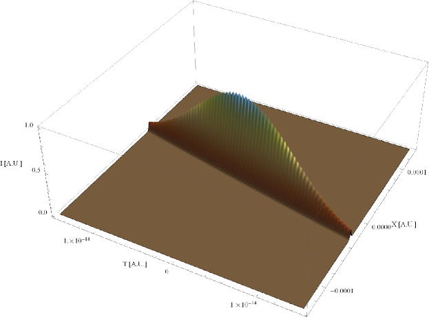
Figure 6: Intensity profile in the space-time domain for $\alpha=100$

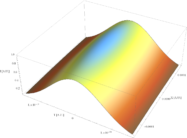
Figure 7: Intensity profile in the space-time domain for $\alpha=0.1$

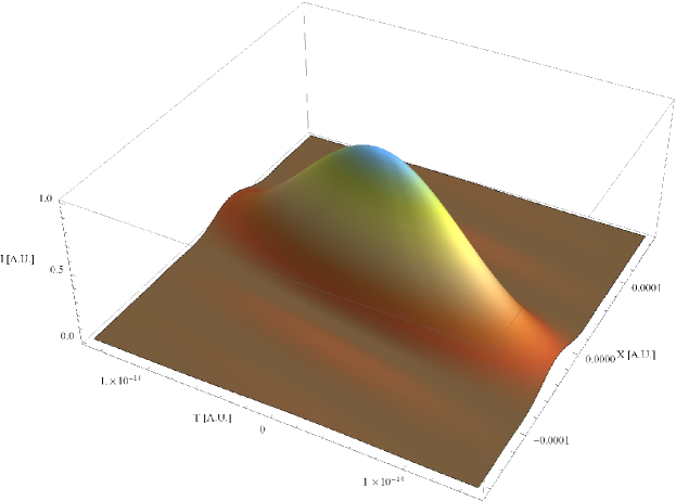
Figure 8: Intensity profile in the space-time domain for $\alpha=2$

Figure 9: Resolving power normalized to the asymptotic case for $\alpha\ll 1$ as a function of $\alpha$.

Figure 10: Transverse spot size of the photon beam normalized to the asymptotic case for $\alpha\gg 1$ as a function of $\alpha$. We assume that the magnification of the two-lens optical system of the monochromator compensates the astigmatism introduced by the grating, that is $f\theta_{i}/f^{\prime}\theta_{D}=1$.

We fix the slit function $S$ as

$$S(x)=1~{}~{}\mathrm{for}~{}|x|<d_{s}$$ (35)

$$S(x)=0~{}~{}\mathrm{for}~{}|x|>d_{s}$$ (36)

Given a slit with half size $d_{s}$, we introduce a normalized notion of slit size

$$\alpha=\frac{d_{s}}{\sigma_{f}}=d_{s}\frac{k\sigma}{\beta f}$$ (37)

We can now plot the intensity profile in the space-time domain for different values of the normalized slit size $\alpha$. Fig. 6 and Fig. 7 qualitatively show the two limiting situations respectively for $\alpha=100$ and $\alpha=0.1$. The spatiotemporal coupling is evident in Fig. 6. Fig. 8 shows the analogous plot in an intermediate situation, for $\alpha=2$.

It is possible to show the output characteristics of the radiation as a function of the slit size by means of universal plots. We first consider the resolving power $R=(\Delta\omega/\omega)^{-1}_{\mathrm{FWHM}}$. We introduce the resolving power $R_{n}$ normalized to the inverse of the maximal bandwidth in Eq. (24), that is the bandwidth in the limiting case for $\alpha\ll 1$, as

$$R_{n}=R\left(\frac{1.18\theta_{i}d}{2\pi\sigma}\right)~{}.$$ (38)

The behavior of $R_{n}$ as a function of $\alpha$ is shown in Fig. 9. The resolution of monochromator increases as the slit size decreases. The $90\%$ of the maximal resolution level is met for normalized slit width less than $\alpha<1$. However, the energy of the seed pulse decreases proportionally to the decrease of the slit width. Moreover, decreasing the slit width will also cause an increase of the output beam size. This will lead to spatial mismatch between the seed beam and the FEL mode in the second undulator. The relationship between the beam transverse size (in terms of FWHM) and slit width is shown in Fig. 10, where we plot the transverse spot size of the photon beam normalized to the asymptotic case for $\alpha\gg 1$ as a function of $\alpha$. To summarize, it is not recommended that the normalized slit width be narrower than unity if a reasonable seed field amplitude is required.

Finally, a useful figure of merit measuring the spatiotemporal coupling can be found in GABO . Considering the angular dispersion this parameter can be written as

$$\rho=\int dk_{x}d\Delta\omega I(k_{x},\Delta\omega)\frac{k_{x}\Delta\omega}{<(\delta k_{x})^{2}>^{1/2}<(\delta\omega)^{2}>^{1/2}}~{},$$ (39)

where

$$<(\delta k_{x})^{2}>=\int dk_{x}d\Delta\omega I(k_{x},\Delta\omega)k_{x}^{2}~{},$$ (40)

$$<(\delta\omega)^{2}>=\int dk_{x}d\Delta\omega I(k_{x},\Delta\omega)\Delta\omega^{2}~{},$$ (41)

$$I(k_{x},\Delta\omega)=|E(k_{x},\Delta\omega)|^{2}$$ (42)

The range of $\rho$ is in $[-1,1]$ and readily indicate the severity of these distortions.

Figure 11: Dependence of the spatiotemporal coupling as a function of $\alpha$ as from Eq. (39).

To estimate the pulse front tilt distortion calculate the pulse front tilt parameter $\rho$ as a function of the slit width $\alpha$. The results are shown in Fig. 11. It is found to be larger than $50\%$ for a slit width $\alpha>1$. Therefore, standard tuning of the seed monochromator will lead to significant spatiotemporal coupling in the seed pulses. The effect of pulse front tilt distortion can be reduced if the slit width will be narrower than $\alpha<1$. However, the reduction of the pulse front tilt influence is accompanied by significant loss in seed signal amplitude.

4 Conclusions

To the best of our knowledge, there are no articles reporting on the impact of pulse front tilt distortions of the seed pulse in the performance on self-seeding soft X-ray setups. Spatiotemporal coupling is natural in grating monochromator optics, because the monochromatization process involves the introduction of angular dispersion, which is equivalent to pulse front tilt distortion. In general, it is desirable that the resulting seed pulse be free of such distortion. This can be achieved only by decreasing the width of the monochromator slits. On the one hand, decreasing the slit width increases the resolving power and suppresses the pulse front tilt distortion. On the other hand, it decreases the seed power and increases the transverse mismatch with the FEL mode in the second undulator. As a result, a tradeoff must be reached between achievable resolution and effective level of the input signal.

Transverse coherence of XFEL radiation is settled without seeding. This is due to the transverse eigenmode selection mechanism: roughly speaking, only the ground eigenmode survives at the end of amplification process. It follows that the spatiotemporal distortions of the seed pulse do not affect the quality of the output radiation. They only affect the input signal value. Therefore, the relevant value for self-seeded operation is the input coupling factor between the seed pulsed beam and the ground eigenmode of the FEL amplifier.

In order model the performance of a soft X-ray self-seeded FEL with a grating monochromator, one naturally starts with the grating monochromator optical system. One aspect of optimizing the output characteristics of the self-seeded FEL involves the specification of spectral width, peak power, pulse-front tilt parameter and transverse size of the seed pulse as a function of the slit width. This can be achieved by purely analytical methods. Another aspect of the problem is the modeling of the FEL process including a seed pulse with spatio-temporal distortions and transverse mismatching with the ground FEL eigenmode. This study can be made only with numerical simulation code.

In this article we restrict our attention to the first part of the self-seeding process, discussing spatiotemporal coupling of the electric field in seed pulses. The field amplitude at the exit of the self-seeding grating monochromator can be obtained using physical optics rather than a geometrical approach. An analysis of the behavior of an X-ray optical pulse passing through a grating monochromator is given in terms of analytical results. In order to make results useful for practical applications, we have included numerous universal graphs which can be useful to find a balance between resolving power, seed power and pulse quality during the design phase.

5 Acknowledgements

We are grateful to Massimo Altarelli, Reinhard Brinkmann, Serguei Molodtsov and Edgar Weckert for their support and their interest during the compilation of this work.

References

- [1] J. Feldhaus et al., Optics. Comm. 140, 341 (1997).
- [2] E. Saldin, E. Schneidmiller, Yu. Shvyd’ko and M. Yurkov, NIM A 475 357 (2001).
- [3] E. Saldin, E. Schneidmiller and M. Yurkov, NIM A 445 178 (2000).
- [4] R. Treusch, W. Brefeld, J. Feldhaus and U Hahn, Ann. report 2001 ”The seeding project for the FEL in TTF phase II” (2001).
- [5] A. Marinelli et al., Comparison of HGHG and Self Seeded Scheme for the Production of Narrow Bandwidth FEL Radiation, Proceedings of FEL 2008, MOPPH009, Gyeongju (2008).
- [6] G. Geloni, V. Kocharyan and E. Saldin, ”Scheme for generation of highly monochromatic X-rays from a baseline XFEL undulator”, DESY 10-033 (2010).
- [7] Y. Ding, Z. Huang and R. Ruth, Phys.Rev.ST Accel.Beams, vol. 13, p. 060703 (2010).
- [8] G. Geloni, V. Kocharyan and E. Saldin, ”A simple method for controlling the line width of SASE X-ray FELs”, DESY 10-053 (2010).
- [9] G. Geloni, V. Kocharyan and E. Saldin, ”A Cascade self-seeding scheme with wake monochromator for narrow-bandwidth X-ray FELs”, DESY 10-080 (2010).
- [10] Geloni, G., Kocharyan, V., and Saldin, E., ”Cost-effective way to enhance the capabilities of the LCLS baseline”, DESY 10-133 (2010).
- [11] Geloni, G., Kocharyan V., and Saldin, E., ”A novel Self-seeding scheme for hard X-ray FELs”, Journal of Modern Optics, DOI:10.1080/09500340.2011.586473
- [12] J. Wu et al., ”Staged self-seeding scheme for narrow bandwidth , ultra-short X-ray harmonic generation free electron laser at LCLS”, proceedings of 2010 FEL conference, Malmo, Sweden, (2010).
- [13] G. Geloni, V. Kocharyan and E. Saldin, ”Scheme for generation of fully coherent, TW power level hard x-ray pulses from baseline undulators at the European XFEL”, DESY 10-108 (2010).
- [14] Geloni, G., Kocharyan, V., and Saldin, E., ”Production of transform-limited X-ray pulses through self-seeding at the European X-ray FEL”, DESY 11-165 (2011).
- [15] W.M. Fawley et al., Toward TW-level LCLS radiation pulses, TUOA4, to appear in the FEL 2011 Conference proceedings, Shanghai, China, 2011
- [16] J. Wu et al., Simulation of the Hard X-ray Self-seeding FEL at LCLS, MOPB09, to appear in the FEL 2011 Conference proceedings, Shanghai, China, 2011
- [17] Y. Feng et al., ”Optics for self-seeding soft x-ray FEL undulators”, proceedings of 2010 FEL conference, Malmo, Sweden, (2010).
- [18] Y. Feng, at al. ”Compact Grating Monochromator Design for LCLS-I Soft X-ray Self-Seeding”, https://sites.google.com/a/lbl.gov/realizing-the-potential-of-seeded-fels-in-the-soft-x-ray-regime-workshop/talks
- [19] G. Geloni, V. Kocharyan and E. Saldin, ”Self-seeding scheme for the soft X-ray line at the European XFEL”, DESY 12-034 (2012).
- [20] A. M. Weiner. Ultrafast Optics. Wiley, New Jersey, 2009
- [21] J. Hebling, ”Derivation of the pulse front tilt caused by angular dispersion”, Opt. Quantum Electron. 28, 1759 (1996)
- [22] G. Pretzler, et al., Appl. Phys. B 70, 1-9 (2000)
- [23] R. R Lindberg and Y. V. Shvyd’ko, ”Time dependence of Bragg forward scattering and self-seeding of hard x-ray free-electron lasers”, http://arxiv.org/abs/1202.1472
- [24] P. Gabolde et al., ”Describing first-order spatio-temporal distortions in ultrashort pulses using normalized parameters”, Optics Express 15, 242 (2007)